Revisiting Rebound Effects from Material Resource Use. Indications for Germany Considering Social Heterogeneity

Abstract

In contrast to the original investigation by William Stanley Jevons, compensations of energy savings due to improved energy efficiency are mostly analyzed by providing energy consumption or greenhouse gas emissions. In support of a sustainable resource management, this paper analyzes so-called rebound effects based on resource use. Material flows and associated expenditures by households allow for calculating resource intensities and marginal propensities to consume. Marginal propensities to consume are estimated from data of the German Socio-Economic Panel (SOEP) in order to account for indirect rebound effects for food, housing and mobility. Resource intensities are estimated in terms of total material requirements per household final consumption expenditures along the Classification of Individual Consumption according to Purpose (COICOP). Eventually, rebound effects are indicated on the basis of published saving scenarios in resource and energy demand for Germany. In sum, compensations due to rebound effects are lowest for food while the highest compensations are induced for mobility. This is foremost the result of a relatively high resource intensity of food and a relatively low resource intensity in mobility. Findings are provided by giving various propensity scenarios in order to cope with income differences in Germany. The author concludes that policies on resource conservation need to reconsider rebound effects under the aspect of social heterogeneity.

1. Introduction

The comprehension of rebound effects evolved over time. In the beginning, Jevons [1] stated in his Coal Question from 1865 that “it is wholly a confusion of ideas to suppose that the economical use of fuel is equivalent to a diminished consumption. The very contrary is the truth. As a rule, new modes of economy will lead to an increase of consumption [...]”. Rediscovered by Brookes and Khazoom, it was postulated that “[...] there is no evidence that using energy more efficiently reduces the demand for it” [2].

Most commonly, the understanding of rebound effects stemming from a more efficient use of a certain technology prevails throughout the literature. In energy or conservation economics, rebound effects are analyzed on the basis of substitution and income effects. Assuming that efficiency gains lead to diminishing marginal costs and therewith leading to lower prices for the commodity at stake, substitution effects lead to an increase in consumption of the good. This is referred to as a direct rebound effect. These effects are estimated with up to 30% for energy (heating, cooling) and personal transport commodities [3]. Most uncertain are estimates of indirect effects, which occur when monetary savings are not reinvested in the consumption of the same good, but are invested indirectly in other goods. These estimates range from barely significant to backfire depending on the system of consumption observed and the method applied [4]. An increase of real income due to monetary savings leads most likely to an increase in consumption due to income effects. This holds true for every resource, not just energy. Every action that responds to savings in resources [5] is prone to rebound effects. That ‘action turn’ in the analysis of rebound effects responds to potential behavioral (or systemic) changes in resource conservation.

Eventually, following Sorrell, rebound effects may be understood as “the unintended consequences of actions by households to reduce their energy consumption and/or greenhouse gas (GHG) emissions” [6]. Then, it is no matter of efficient, consistent or sufficient sustainable actions. It basically does not matter for the analysis of effects if, for instance, more efficient light bulbs are plugged in, a candle is lit up or the lights stay just switched off. In any case, monetary savings occur and rebound effects are most likely to be observed. For the latter, no substitution effect is supposed to occur in the short run, since switching off the lights is unlikely to change prices unless these actions do not accumulate for economy wide rebound effects [7]. I adapt Sorrels definition with replacing “energy consumption and/or greenhouse gas emission”, but orientate on resource use in terms of total material requirement (TMR) [8] per capita in consumption.

The article presents a basic methodological approach on how to account for complexities like recent studies tried to cope with when dealing with indirect rebound effects [9]. The paper focuses on material requirements for food, housing and mobility, which are most relevant when it comes to the consumption of resources by private households [10,11]. Hence, I am able to reduce complexity in consumption patterns without foregoing relevant material requirements of households. In addition, I control for social heterogeneity by differentiating the results between low and high incomes. My approach follows Jevons, addressing rebound effects in the light of material resource use. I start by giving basic methodological considerations. The methodological section is followed by giving the formal frame for my analysis, presenting the data sets I require to collect and combine in order to illustrate the basic approach. I conclude on principles at which the estimations hint, discuss methodological shortcomings and the interpretation of results.

2. Methodology

When talking about rebound effects, it always comes to the notion of utility that is based on consumption. Preferences of a utility maximizing representative agent whose utility function solely depends on consumption of goods are considered as given. From a sociological perspective, preferences may change over time, such that gains in efficiency do not increase consumption, but may be spent in leisure time. Nevertheless, I cannot look into the black box of preferences, but want to put further research on the enquiry of the viability of preferences to better understand why rebound effects occur (see [12]).

I assume weak separability of preferences by consumers between the aggregated fields of consumption. That means that consumers keep budgets separated for each category of consumption, e.g., preferences for commodities for food are independent of preferences for transport: In a first stage, consumers keep budgets for commodity groups, in the following stages, preferences for goods within groups are formulated. Preferences between groups are independent of preferences for goods within groups. This holds true when the stages on budgeting are independent from each other. For this to be justified, I assume that the results of so-called multi-staged budgeting equal single-stage budgeting with perfect information of agents. That makes an aggregated Input/Output(I/O)-approach econometrically feasible, widely adopted and common when it comes to the analysis of indirect effects [4].

I aggregate commodities within consumption categories such that I end up with food, housing and mobility. I regress income on expenditures in the aggregated groups of consumption such that I refer to marginal propensities to consume (see Equation (2) in Section 2.2). When adding up expenditures, they do not exceed budget constraints (adding-up restriction). The same accounts for propensities, which do not exceed unity. Eventually, I aggregate for linear Engel curves (see Equation (3) in Section 2.2).

Furthermore, I assume that savings in resource use equal cost reductions for the service provided. In turn, decreasing marginal total costs induce direct as well as indirect effects due to changes in real income by consumers [13]. According to Slutksky, both substitution and income effects lead to an increase in utility and thus an increase in consumption. I do not explicitly describe those mechanisms, but would rather refer to basic neoclassic microeconomics in order to keep the analysis feasible and comprehensible (for an extensive introduction see [4]).

By describing indirect effects, I combine technological with behaviorally pulled savings in socio-technical systems. It is reasonable that socio-technically induced changes will always lead to indirect effects. For instance, savings from food will most likely be re-spent for other commodities than those in which the savings occur. That is why I consider income effects relevant for describing the effects reliably.

2.1. Resource Use and Resource Intensities

The consumption in food, housing and transport accounts for 80% of total material requirements (TMR) of private households in Germany [14]. In absolute terms, nearly 30 t per person and year crop up in these three arrays according to the Classification of Individual Consumption of Purpose (COICOP) [14].

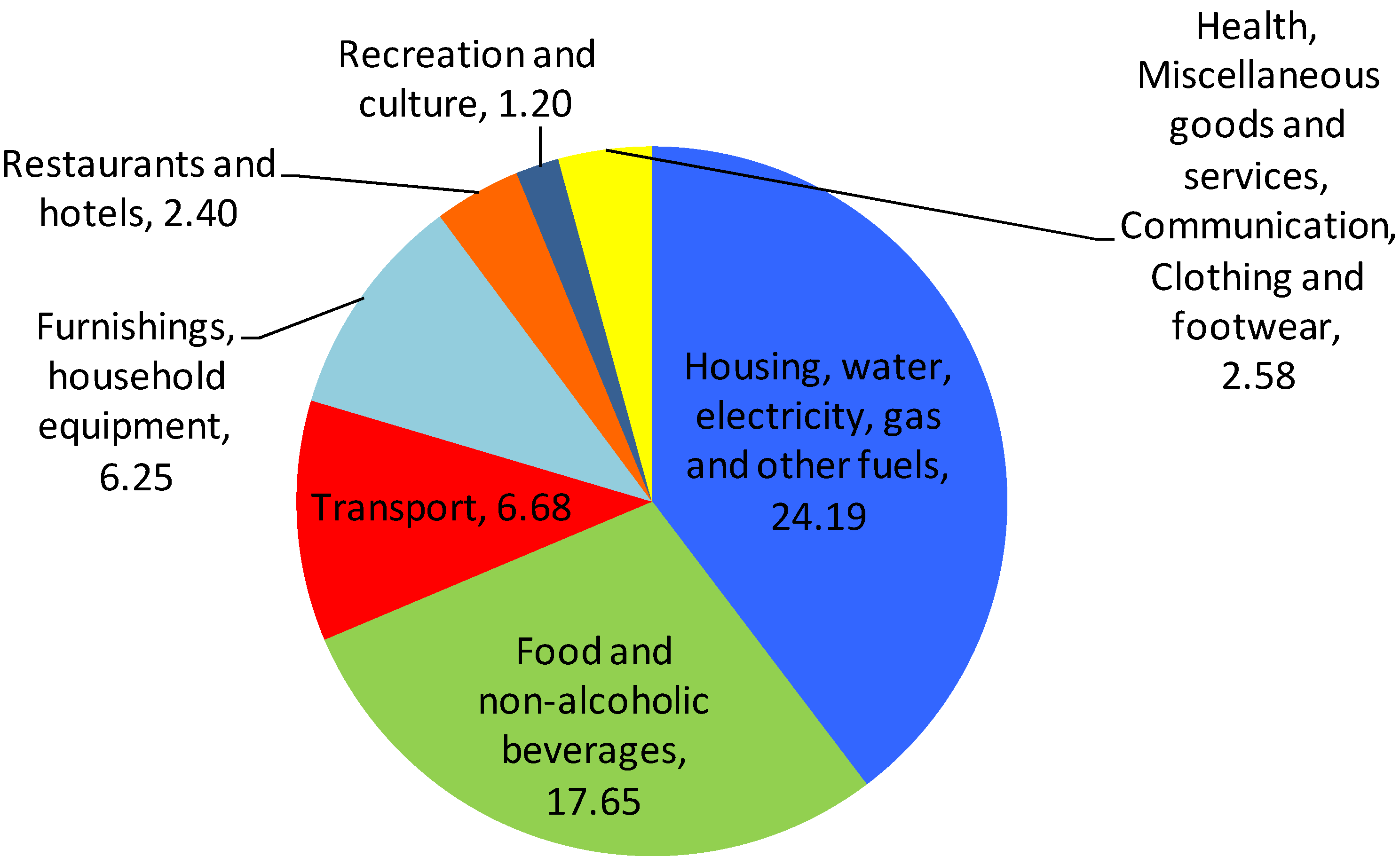
Figure 1 shows the resource use per household in Germany for 2005. Categories, which account for less than 1% of overall consumption are summarized and added up. These are “Health”, “Miscellaneous goods and services”, “Communication”, “Clothing and footwear”, “Alcoholic beverages, tobacco and narcotics” and “Education”.

Figure 1. Total material requirements (in t) induced by direct and indirect consumption of private households in Germany for 2005.

Figure 1. Total material requirements (in t) induced by direct and indirect consumption of private households in Germany for 2005.

Source: Own depiction using [14].

In monetary terms, 50% of the final consumption expenditures of private households (HFCE) are spent for food, housing and transport [15]. When comparing resource use (in kg) and household final consumption expenditures (in Eurocent), I can derive the average resource intensity RI. In general, j stands for the considered field of final consumption expenditures C. In my analysis, I focus on food, housing and mobility, depicted as transport in COICOP [15].

RI_j = TMR_j/C_j

(1)

The direct material input (DMI) in 2005 for food is 1.8 kg DMI per Euro spent in the EU-27, for housing and mobility it is 0.7 kg per Euro spent. The DMI refers to the amount of materials directly used in the economy. In addition to DMI, TMR includes the so-called material footprints. Those consist of unused domestic extraction like overburden from coal mining, excavated soil for constructions or soil erosion in agriculture. In addition, TMR includes all foreign life cycle wide required materials—used and unused—which were necessary to provide an imported good. These are commonly referred to as indirect material flows. TMR thus constitutes the most comprehensive input oriented indicator and represents the magnitude of potential environmental pressure exerted by the extraction and use of natural resources [16,17]. Accordingly, the resource use and resource intensities in terms of TMR per Euro are higher than in terms of DMI per Euro. In Germany, the RI accounts 5.1 kg per Euro for food, 3.2 kg per Euro for housing and 1.5 kg per Euro for mobility (2005) [own calculations using unpublished results of an input-output analysis on environmental pressures from European consumption and production, personal communication from J. Acosta-Fernández and H. Schütz (2011) for [11].

The (dis)advantage of I/O-analysis is its level of aggregation. Here, a trade-off between differentiation and comprehension is inevitable. Looking at inputs and outputs as a whole does comprise and show all material flows of a system, while I am not able to differentiate within the categories at stake. For instance, I do not know the specific intensities for mobility by air or by car. Kotakorpi et al. [18] assume significant differences in terms of abiotic material input per passenger-km between concerning modes of private transport with mobility by car (2.02 kg) having the highest input in contrast to train (1.2 kg), bicycle (0.38 kg) or long-haul flights (0.06 kg). In the following, I assume that modes of transport equal in intensities. Hybrid analysis combining LCAs of specific commodities and corresponding inputs and outputs of environmental pressures allows to differentiate between the commodities observed and to vary the aggregation accordingly. The hybrid approach is very data intensive and less feasible, such that studies on indirect effects rely merely on I/O-analysis [19].

2.2. Marginal Propensities to Consume

The second essential variable I have to introduce are marginal propensities to consume (MPC). These are defined as the proportion of the marginal change in disposable income Y which individual i spends in field j of consumption C, that is:

MPC_ij = ∂C_ij/∂Y_i

(2)

In order to observe marginal propensities to consume econometrically, I calculate multiple multivariate linear regressions. Approaching indirect rebound effects by estimating MPCs econometrically is derived and adopted from Alfredsson [20].

The model may be formally noted as:

(3)

whereas E_n are the expenditures of the ith observation, depending on the yth income [21] in the sample with L being a vector of potential covariates influencing the expenditures of the ith observation. The numbers represent the Cs fields of consumption up to n in multiple regressions, in Equation (2) noted as j. The regression coefficients β_yn show the marginal propensities to consume in the n given fields of consumption. For the estimation of marginal propensities to consume, no covariates are introduced so far. The introduction of additional variables that explain the marginal propensities to consume should follow a concise theoretical argumentation from the perspective of behavioral and social sciences, which is missing so far when it comes to the empirical estimation of rebound effects [22]. It is up to future analysis to introduce covariates in order to offer further insight into the emergence and heterogeneity of indirect rebound effects.

2.3. Rebound Effects in Resource Use

Having calculated resource intensities and marginal propensities to consume, I am able to integrate them for the estimation of rebound effects. First, I calculate the engineered savings in the fields of consumption by applying the relative scenario savings s (described in Chapter 3) on expenditures per capita. Engineered savings are the expected savings in resource use by consumers (TMR_ENGij). Actual resources that are used per capita i is the product of spending c and js average resource intensities RI (here for food, housing and mobility) (Equation (4)). Expected savings r are calculated by multiplying the proposed savings in spending c by its average resource intensities (Equation (5)). The engineered savings are then the subtraction of the expected savings r in resource use with the actual resource use in the specific fields of consumption (Equation (6)).

TMR_ij = c_ij × RI_j

(4)

and

r_EXPij = (c_ij − c_ij × s_j) * RI_j

(5)

in:

TMR_ENGij = r_EXPij − TMR_ij

(6)

In order to calculate direct and indirect effects, I need to reconsider the calculated MPCs and combine them with the resource use calculated above. Direct effects occur when savings according to the anticipated MPCs are invested in the same field of consumption where the monetary gains occur. Indirect effects occur, if the monetary gains are reinvested indirectly in other fields of consumption observed. Eventually, I note for direct and indirect effects from re-spending in absolute terms

TMR_REBij = r_EXPij × MPC_ij

(7)

Relative rebound effects (in percent) are then the compensation of re-allocated resource use according to MPCs in relation to engineered savings.

(8)

3. Identifying Experimental Scenarios on Savings

Before describing the sets of data used, I derive savings s in material resource use from scenarios of recent literature. I do not fully describe and compare the studies, but rather extract an elaborated guess on how the use of resources and energy alike may decrease in the future. Distelkamp et al. [23] simulate a sectorally disaggregated model for potentials in resource efficiency. They consider economic policy instruments like changes in value added taxes for transport services or a resource tax for the building sector. Regulatory instruments discuss the rules for recycling of specific non-ferrous metals. Information instruments simulate the introduction of technological best practice to firms under conditions of perfect knowledge on the market. In sum, the potential of a forced policy for resource efficiency is estimated to drop by 20% in total material requirement until 2030. Still, adequate simulations of disaggregated demand of private households are missing. Therefore, I add references to scenarios on energy savings. These are not identical to savings in resource use but may correlate to savings in resource use since usage, i.e., energy consumption, is decisive for resource use by private households [24].

Concerning housing, I focus on retrofitting rates and replacement of heating systems since these account for 80% of savings in private households. Besides variables concerning the mix of used energy, the increase of passive house construction, the rate of retrofitting is decisive [25]. Ambitious efficiency scenarios assume the rewards of optimal efficiency gains. In ambitious scenarios, the rate of retrofitting increases up to 1.3% until 2020. The replacement rate of efficient heating systems is supposed to rise to 4% per anno, compared to 3.3% in the reference system. The system of reference resembles frozen efficiency gains for Germany under predominant economic conditions for 2007. Other savings are subsumed under efficient appliances. In sum, efficiency gains account for 15% ([26] own calculations). These findings are in line with corresponding energy scenarios for Germany. Here scenarios suggest savings in used energy of 13% compared to 2008, suggesting an efficiency rate of 2.5% for the considered scenarios [27]. These are in turn equal to an extrapolation of the efficiency rate of the energy efficiency index of households (ODEX [28] between 2000 and 2007 [29]. Other ambitious efficiency models suggest a reduction of used energy by private households of 17% for gas and 13% for electricity in 2020 compared to 2000. Here again, saved used energy for heating accounts for 14% [30]. I calculate the relative savings proportionally to savings in used energy. A gain in efficiency equals an equivalent drop in costs for costumers (see assumptions in Section 2). For savings in energy and resource use, I therefore conclude a drop in costs by 15% for customers in housing.

Concerning mobility, efficiency gains are in first place due to the introduction of efficient cars and their efficient use. Savings are that significant, because federal norms are pretty weak with 133.6 g CO₂/km for 2020, an ambitious efficiency scenario aims at 105 g CO₂/km, which is still 10 g above the aimed EU norms for 2020. Efficient cars account for 12% in the transport system and efficient use for another 11%. The switch to public transportation accounts only for 3%. In sum, efficiency gains will account for 26% in 2020 [31]. These may be valid since models of the environmental agency in Germany suggest efficiency gains in transportation of 24% [32]. I calculate a drop in costs for private mobility of 25%.

For food consumption, no socio-technological efficiency gains are assumed, but a more efficient use of foodstuffs. Here, efficiency refers to the demand of foodstuffs in relation to its specific intake of calories. A range of literature assessed the life cycle wide energy consumption and emission patterns from foodstuff to diets. In core, studies suggest that a vegetarian diet or a diet foregoing the consumption of animal products potentially contributes highest for a reduction of energy consumption and emissions. Jungbluth et al. [33] predict that a vegetarian diet will reduce emissions compared to reference food consumption in Switzerland by more than 25%. This is in accordance with reductions proclaimed by Macdiarmid et al. [34] in the livewell UK report for 2020 and for Sweden in 2020 as described by Alfredsson [20]. I assume the same for Germany, calculating a drop in costs for foodstuffs by 25%. These are the basic scenarios I apply in order to illustrate my estimations on rebound effects.

4. Data

The data on material flows has already been introduced by describing resource use and the calculation of resource intensities in Section 2.1. The data for expenditures are derived from the Socio-Economic Panel in Germany (SOEP). Since expenditures on energy and resources are only available for households, the social differentiation is limited to available data on the level of households that do not encompass data on age, gender or similar common, temporary fixed characteristics that are supposed to be controlled for when structuring the results in social terms. The SOEP allows observing for expenditures in the three respected fields of consumption for 2003. A calculation of differences in MPCs across the years was not possible. Panel data would have been required for the expenditures at stake rather than reliance on cross-sectional data.

The item on food consumption asks for expenditures on groceries per week. The proxy on spending for housing is monthly expenditures on heat and energy for oil, gas, coal, electricity and/or heat with district heating. I complemented expenditures on housing by adding yearly expenditures on maintenance. When it comes to mobility, some shortcomings occur due to a suboptimal set of variables that only covers private mobility by car. Here, for every car in the household, I know the driven kilometers per year and the fuel consumption per 100 km. In order to get the costs of private mobility, I impute the average costs per liter gas in the year 2003 in Germany that was 1.53 €/L according to data of the Federal Statistical Office. The average fuel consumption per 100 km in households with up to three cars is 7.4 L/100 km. In sum, the average cost for mobility per capita per year in 2003 is approximately 1,788 Euro. In order not to overestimate the consumption of the second and third vehicles, the average fuel consumption in households is calculated by weighting the consumption of the vehicles with their specific kilometers driven in the sample. In general, I only consider observations for the estimation that actually show expenditures, all others are set to zero or missing expenditures when the item does not apply to the household.

So far, I have observed discrepancies between the aggregation of resource use and variables on costs according to COICOP. The specific proxy for mobility regarding kilometers driven per vehicle in a household seems to be the most precarious factor. Since there is no reliable data on material footprints of specific transport modes available, I follow the common literature on rebound effects relying merely on the relevance of private mobility by car when dealing with effects on mobility [35].

I consider savings to have no direct impact on resource use. Druckman et al. [9] describe low rebound effects from savings having low impact on rebound effects when varying saving rates significantly. Less than 10% of the observed variance of overall effects stem from severe changes in savings from −4% to 100%. I simplify these results by assuming that marginal propensities to save do not inherit rebound effects. Concerning the relation between propensities to consume and to save, Stein [36] shows that between 1995 and 2007 in the SOEP on average, 90% of income accounts for spending and 10% accounts for savings. In sum, the statistical proxies range from expenditures on groceries, energy (electricity, heat, maintenance) to private car use for resource use of food, housing and mobility (see Table 1).

Since the SOEP claims to offer representative data for Germany, it makes sense to see if my sample of the SOEP offers the same. Two sample t-tests show significant differences between the households for which I estimate MPCs and the complete SOEP sample of households for annual income, expenditures on food and mobility, but not for housing. The average net income per year is higher (33,183 Euro vs. 25,914 Euro), so are the average expenditures on food (4,684 Euro vs. 6,125 Euro) and mobility (2,179 Euro vs. 2,031 Euro). Only for housing is the probability that households in the sample at stake have higher expenditures just slightly above 50% (3,495 Euro vs. 3,484 Euro). The households for which I compute MPCs have higher incomes and higher expenditures in the fields of consumption concerned.

Table 1. Description of used and generated variables.

Variable	Obs.	Mean	Range	Std. Dev.
Fuel Consumption per 100 Km of 1st Vehicle	4,472.00	8.40	39	1.83
Fuel Consumption per 100 Km of 2nd Vehicle	1,744.00	7.68	24	2.14
Fuel Consumption per 100 Km of 3rd Vehicle	371.00	6.85	19	2.58
Km Per Year of 1st Vehicle	4,553.00	14,521.95	217,990	11,603.75
Km Per Year of 2nd Vehicle	1,774.00	12,367.91	258,990	12,023.24
Km Per Year of 3rd Vehicle	383.00	8,655.95	49,970	8,426.31
Costs of Mobility	5,753.00	1,788.08	31,409.48	1,936.55
Maintenance Costs in Previous Year	1,853.00	3,819.13	169,985	9,417.33
Annual Expenditures on Oil	1,067.00	1,039.47	5,960	557.84
Annual Expenditures on Gas	988.00	1,009.62	3,723	535.48
Annual Expenditures on District Heating	140.00	744.50	2,391	426.86
Annual Expenditures on Electricity	1,609.00	681.54	3,591	421.73
Annual Expenditures on Coal, Wood	315.00	317.89	1,991	312.12
Annual Expenditures on Other	47.00	807.81	2,141	716.58
Costs of Housing	3,015.00	3,490.02	169,991	7,655.41
Groceries Estimated Euros Per Month	2,995.00	450.35	2,491	244.57
Household Net Income	5,495.00	2,319.61	19,991	1,290.54

Table 1. Description of used and generated variables.

Variable	Obs.	Mean	Range	Std. Dev.
Fuel Consumption per 100 Km of 1st Vehicle	4,472.00	8.40	39	1.83
Fuel Consumption per 100 Km of 2nd Vehicle	1,744.00	7.68	24	2.14
Fuel Consumption per 100 Km of 3rd Vehicle	371.00	6.85	19	2.58
Km Per Year of 1st Vehicle	4,553.00	14,521.95	217,990	11,603.75
Km Per Year of 2nd Vehicle	1,774.00	12,367.91	258,990	12,023.24
Km Per Year of 3rd Vehicle	383.00	8,655.95	49,970	8,426.31
Costs of Mobility	5,753.00	1,788.08	31,409.48	1,936.55
Maintenance Costs in Previous Year	1,853.00	3,819.13	169,985	9,417.33
Annual Expenditures on Oil	1,067.00	1,039.47	5,960	557.84
Annual Expenditures on Gas	988.00	1,009.62	3,723	535.48
Annual Expenditures on District Heating	140.00	744.50	2,391	426.86
Annual Expenditures on Electricity	1,609.00	681.54	3,591	421.73
Annual Expenditures on Coal, Wood	315.00	317.89	1,991	312.12
Annual Expenditures on Other	47.00	807.81	2,141	716.58
Costs of Housing	3,015.00	3,490.02	169,991	7,655.41
Groceries Estimated Euros Per Month	2,995.00	450.35	2,491	244.57
Household Net Income	5,495.00	2,319.61	19,991	1,290.54

5. Results

When I look at the average total resource use of the sample for housing, food and mobility, I observe a median of 51 t of TMR per household within a large range from 7 t to 311 t (see Figure 2). On aggregation, the total material requirement per household sums up to 48 t of TMR encompassing housing, food and mobility in Germany (see Figure 1). In line with the comparison of my sample with the whole SOEP, the sample is likely to present higher total material requirements than average in Germany. The higher average of income and expenditures of private households in the sample observed may affect their propensities to consume and, thus, may show differeing rebound effects from the average for Germany.

5.1. Descriptives of Total Material Requirements

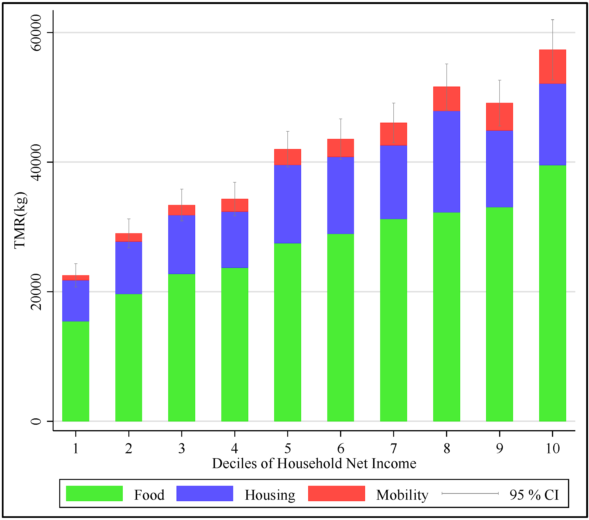
By plotting the average resource use (total material requirement TMR in kg) of food, housing and mobility against deciles of household net income with a 95% confidence interval (CI) (Figure 2), the average resource use rises in total when income rises, except for resource use of the ninth decile. Herein, the expenditures for housing decline stronger than the expenditures for food increase. Resource use for food rises continuously, as does resource use for mobility as income rises. On average, the bars show that resource use is highest for food, followed by housing and transport. When splitting the sample based on average household net income (see Table 1 for mean of household net income), higher incomes show a resource use, which is 1.5 times higher than that of lower incomes. In more detail, the lowest decile shows an average total material requirement of a total of 22.1 t, whereof 15.4 t are for food, 6.4 t for housing and 0.7 t for mobility. The highest decile shows an average total material requirement of a total of 57.2 t, whereof 39.5 t are for food, 14.5 t for housing, and 5.2 t for mobility. Thus, the highest decile shows a resource use, which is 2.6 times higher than in the lowest decile.

Figure 2. Average total material requirements of food, housing, and mobility per deciles of household net income within the sample.

Figure 2. Average total material requirements of food, housing, and mobility per deciles of household net income within the sample.

Source: Own depiction using [14].

5.2. Marginal Propensities to Consume

The descriptives show that resource use per household is relatively high for food. That is due to relative high resource intensities for foodstuffs and relatively high marginal propensities to consume in that array according to the observations in the sample. The coefficients of the multiple regression in Table 2, Table 3 and Table 4 show the MPCs for the whole sample, as well as for relatively low and high household net incomes for food, housing and mobility. The results depict highest MPCs for food for the whole sample, as well as for low and high incomes. For instance, the whole sample shows that 0.16 Euro are spent for food if income rises per 1 Euro. With such a marginal raise in income, 0.09 Euro are expended for housing, but only 0.06 Euro are spent for mobility. MPCs are higher with relatively low incomes for all arrays of consumption. In contrast, MPCs for relatively high incomes are lower than average in the sample. For example, 0.14 Euro are spent for food with high incomes, whereas low incomes spend 0.23 Euro for food with a marginally rising income.

Table 2. Marginal propensities to consume for the whole sample.

Expenditures	Coef.	Std. Err.	t	P > |t|	[95% Conf. Interval]
Food	0.1628854	0.00385	42.31	0.000	0.1553364 0.1704345
Housing	0.0935714	0.0042812	21.86	0.000	0.085177 0.1019659
Mobility	0.0667557	0.0011897	56.11	0.000	0.0644232 0.0690882

Note: Robust standard errors, constant suppressed.

Table 2. Marginal propensities to consume for the whole sample.

Expenditures	Coef.	Std. Err.	t	P > |t|	[95% Conf. Interval]
Food	0.1628854	0.00385	42.31	0.000	0.1553364 0.1704345
Housing	0.0935714	0.0042812	21.86	0.000	0.085177 0.1019659
Mobility	0.0667557	0.0011897	56.11	0.000	0.0644232 0.0690882

Note: Robust standard errors, constant suppressed.

Table 3. Marginal propensities to consume for low incomes.

Expenditures	Coef.	Std. Err.	t	P > |t|	[95% Conf. Interval]
Food	0.2337776	0.0029709	78.69	0.000	0.2279505 0.2396048
Housing	0.1535244	0.0106642	14.40	0.000	0.1326053 0.1744434
Mobility	0.0807332	0.0014739	54.78	0.000	0.0778429 0.0836235

Note: Robust standard errors, constant suppressed.

Table 3. Marginal propensities to consume for low incomes.

Expenditures	Coef.	Std. Err.	t	P > |t|	[95% Conf. Interval]
Food	0.2337776	0.0029709	78.69	0.000	0.2279505 0.2396048
Housing	0.1535244	0.0106642	14.40	0.000	0.1326053 0.1744434
Mobility	0.0807332	0.0014739	54.78	0.000	0.0778429 0.0836235

Note: Robust standard errors, constant suppressed.

Table 4. Marginal propensities to consume for high incomes.

Expenditures	Coef.	Std. Err.	t	P > |t|	[95% Conf. Interval]
Food	0.1448665	0.0041721	34.72	0.000	0.1366813 0.1530517
Housing	0.0823442	0.0044983	18.31	0.000	0.0735204 0.0911679
Mobility	0.0637526	0.0013633	46.76	0.000	0.0610791 0.0664261

Note: Robust standard errors, constant suppressed.

Table 4. Marginal propensities to consume for high incomes.

Expenditures	Coef.	Std. Err.	t	P > |t|	[95% Conf. Interval]
Food	0.1448665	0.0041721	34.72	0.000	0.1366813 0.1530517
Housing	0.0823442	0.0044983	18.31	0.000	0.0735204 0.0911679
Mobility	0.0637526	0.0013633	46.76	0.000	0.0610791 0.0664261

Note: Robust standard errors, constant suppressed.

The differences in MPCs along household net incomes and arrays of consumption significantly affect the heterogeneity of calculated rebound effects.

5.3. Rebound Effects

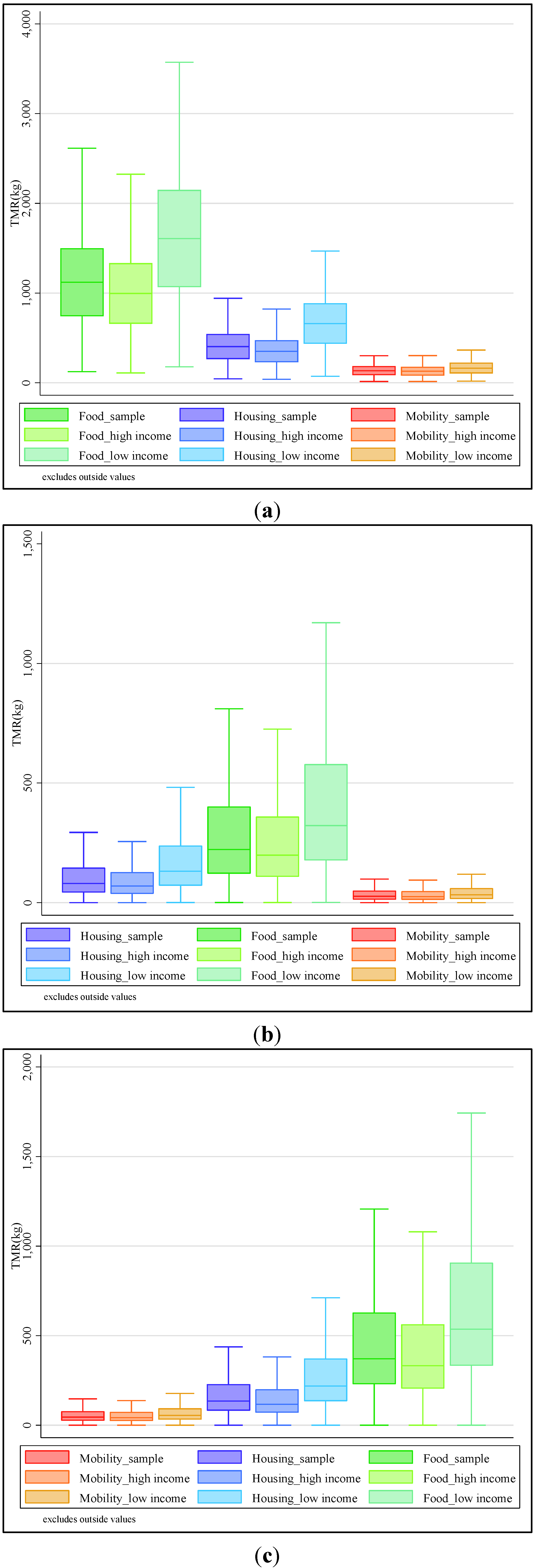
Resulting rebound effects are presented in Figure 3. The box-and-whiskers plots show the median line within the box representing the interquartile range (IQR) that gives the range between the upper quartile (75th percentile) and the lower quartile (25th percentile). The whisker lines of the adjacent values span all data points within 1.5 IQR of the upper and lower quartile. The box-and-whiskers highlight and echo the high variance within the data already depicted in Figure 2.

Figure 3. (a) Rebound effects by resource use for food; (b) Rebound effects by resource use in housing; (c) Rebound effects by resource use in mobility.

Figure 3. (a) Rebound effects by resource use for food; (b) Rebound effects by resource use in housing; (c) Rebound effects by resource use in mobility.

5.3.1. Food

Saving scenarios affect resource use for food relatively strong. When saving a quarter of resource use for foodstuffs, private households save 6877 kg of their total material requirement (TMR) per year (in 2003). Direct rebound effects account for 1120 kg, indirect effects account for 136 kg in mobility and 404 kg in housing for the sample in absolute terms. In this regard, 16% of the assumed savings are compensated by direct effects. Only 8% are compensated indirectly due to re-spending for housing and mobility. When accounting for social heterogeneity in terms of income, re-investment of savings by low incomes in food are 1609 kg, in mobility they are 164 kg and in housing they are 661 kg; for high incomes they are 997 kg in food, 129 kg in mobility and 301 kg in housing. Since the observations only show slight differences in propensities to consume for private mobility, rebound effects are equal here. Overall, 24% of assumed savings in TMR for food are compensated due to rebound effects. Compensations are lower for high incomes, but relatively higher for low incomes. Here, more than one third of the assumed savings is compensated due to rebound effects.

5.3.2. Housing

Potential savings in resource use are comparatively low for housing due to relative inelastic propensities and relatively low resource intensities. When assuming savings of 15% in housing, private households reduce total material requirements by 1665 kg. Direct effects account for 156 kg; savings are reinvested indirectly for consumption in mobility by 53 kg and in food for 431 kg. Here, direct rebound effects are lower than indirect effects. Only 9% of the supposed material savings are compensated directly. But due to re-spending, 29% of the savings are compensated. For low incomes these are 256 kg, 63 kg and 623 kg respectively; for high incomes they account for 156 kg, 50 kg and 386 kg in absolute terms. In total, the rebound effects account for 38% of the whole sample, for low incomes 57% and 35% for high incomes.

5.3.3. Mobility

Savings in mobility are lowest, due to lowest propensities and resource intensity. Here, direct rebound effects compensate for only 56 kg or approximately 7% of the total engineered savings of 842 kg. For high incomes 53 kg, for low incomes 68 kg are compensated directly, this equals 9% and 12% in relative terms. For the sample, 168 kg in housing and 463 kg in food are reinvested, which account for 19% and 54%. For low incomes the numbers are 273 and 668 kg or 32% and 79% in relative terms, for high incomes 146 kg and 414 kg or 17% and 49%, respectively. In sum, rebound effects are highest with 81% of the sample, for low incomes 119% and 73% for high incomes. Low incomes are likely to backfire, since savings are disproportionally reinvested in favor of relatively more resource intensive consumption patterns for housing and food.

5.4. Summary of Results

The estimations show average rebound effects ranging from 24% for food up to 81% for mobility. Heterogeneity in rebound effects shows relatively smaller effects for high incomes and relatively higher effects for low incomes. Low incomes show rebound effects of overall 35% for food up to 119% for mobility. Whereas high incomes show rebound effects of overall 21% for food and up to 75% for mobility. When allowing for re-spending, low incomes are likely to backfire regarding mobility when accounting for resource use (Table 5).

However, admitting that low incomes show higher rebound effects, one has to take into consideration that higher incomes show a total material requirement which is 1.5 times or 51% higher than the TMR of low incomes in the fields of consumption at stake. Considering the heterogeneity of rebound effects estimated in Table 5, the gap in resource use would have been closed for mobility due to the combination of a relative low level of resource use with the highest rebound effects across the fields of consumption and household net incomes. In contrast, the discrepancy in resource use across incomes would only be reduced by 14% by rebound effects in food and by 8% by rebound effects in housing. One has to remember that the higher the average level of income, the higher the average levels of resource use per household (see Figure 2).

Table 5. Average rebound effects in relative and absolute terms for food, housing, mobility for the whole sample, low and high incomes.

Group	Food (%)	Food (kg)	Housing (%)	Housing (kg)	Mobility (%)	Mobility (kg)
Sample	24	1660	38	640	81	687
Low income	35	2434	57	942	119	1009
High income	21	1427	35	592	75	613

Table 5. Average rebound effects in relative and absolute terms for food, housing, mobility for the whole sample, low and high incomes.

Group	Food (%)	Food (kg)	Housing (%)	Housing (kg)	Mobility (%)	Mobility (kg)
Sample	24	1660	38	640	81	687
Low income	35	2434	57	942	119	1009
High income	21	1427	35	592	75	613

6. Conclusions and Discussion

The proposed approach basically combines two benefits when it comes to further research on rebound effects. First, the paper offers estimates on rebound effects in terms of resource use that follows Jevons original discovery of rebound effects. By providing resource use as an accounting scheme for rebound effects, I strive to support sustainable resource management. Second, the method offers an understanding on how rebound effects affect each other indirectly while they open up further research on social heterogeneity. The vast literature on rebound effects concentrates on direct rebound effects due to methodological issues. I do not state to overcome the issues at stake such as dynamics, uncertainties or data incompatibility. On the contrary, the illustrated method implies shortcuts that come with scenarios, cross-sectional analysis and the merge of different sets of data on different levels of aggregation. I mainly suppose that relative savings in energy reduction scenarios correlate with reduction in material resource use. Marginal propensities to consume are calculated cross-sectionally, not accounting for dynamics in propensities over time. Data on resource use is highly aggregated while econometrically, I deal with specific expenditures for cars, groceries and energy use in households. These shortcuts allow only to introduce rebound effects across arrays of consumption in terms of resource use.

The comparison of the results with recent studies on indirect effects is difficult due to the high variance of the results across the studies. When comparing results with the adopted approach from Alfredsson [20] for Sweden, predicted compensations are different across arrays and lower on average for Germany. The findings for food and housing are (in comparison) relatively low, for mobility the estimates tend to backfire when controlling for average income within the sample. That is crucial in order to understand the emergence and implications of indirect rebound effects. These depend on cross-elasticities or propensities to consume across arrays of consumption and their relative resource intensities (see [37] for an argumentation on intensities regarding green house gas emissions). When re-investing savings into relative resource intensive arrays of consumption, an (over)compensation of the engineered savings is likely, always depending on the propensities to consume in the specific array. Then, a relatively low marginal propensity to consume may compensate for the relatively high resource intensity in the given array of consumption. Conversely, high marginal propensities to consume may enforce high resource intensities. In this case, indirect compensations may well go beyond direct effects. These differ significantly when controlling for average income. Concerning the arrays at stake, low incomes are likely to re-spend more monetary savings across the arrays than high incomes.

When aiming at policies to avoid (sic!) rebound effects, social differentiation is crucial in order to anticipate the implications of such policies. In general, policy papers on rebound effects wonder if and how rebound effects may be constrained via flanking policies of efficiency. But sanctioning consumers for (re-)investing savings would eventually result in nudging behavior towards sufficiency and low incomes would be addressed foremost, since the effects are strongest here. At the same time, it is crucial to reconsider that average levels of resource use increase as incomes of private households increase. Considering the results above, this would affect low incomes disproportionally. In such a case, policies on energy conservation need to reconsider rebound effects in terms of social justice and compensation.