A New Composite Index for Greenhouse Gases: Climate Science Meets Social Science

Centre for Efficiency and Productivity Analysis (CEPA), School of Economics, University of Queensland, Brisbane 4072, QLD, Australia
*
Author to whom correspondence should be addressed.
Resources 2017, 6(4), 62; https://doi.org/10.3390/resources6040062
Submission received: 10 August 2017
/
Revised: 13 October 2017
/
Accepted: 20 October 2017
/
Published: 25 October 2017
(This article belongs to the Special Issue Sustainability Indicators for Environment Management)
Abstract
:Global greenhouse gas emissions have increased at a rate of nearly 2% per year since 1970, and the rate of increase has been increasing. The contribution of greenhouse gases to global warming constitutes an environmental management challenge requiring interdisciplinary effort and international cooperation. In an effort to meet this challenge, the Kyoto Protocol imposes limits on aggregate CO2-equivalent emissions of four greenhouse gases, although it permits countries to trade off one gas for another at specified rates. This requires a definition of trade-off rates, which the Protocol specifies as Global Warming Potentials, although these have been controversial since their introduction. The primary source of concern has been the constancy of the trade-off rates, both across countries and through time. We propose a new composite index that allows freely variable trade-off rates, thereby facilitating the design of efficient abatement policy. In a pair of exercises we compare our composite index with that used by the Protocol. In both exercises we reject the constancy of trade-off rates, although despite the significantly different weighting schemes we find a degree of concordance between the two greenhouse gas indices.
1. Introduction
The Intergovernmental Panel on Climate Change (IPCC) tracks the growth of anthropogenic greenhouse gas emissions. The Fifth Assessment Report of 2013–2014 claims “with high confidence” that about half of the cumulative emissions between 1750 and 2011 have occurred in the last 40 years, with about 40% of cumulative emissions remaining in the atmosphere and continuing to contribute to global warming. Emissions have grown at a rate of 1.7% per annum since 1970, and the growth rate has increased to 2.2% per annum since 2000, despite increasing mitigation efforts and the depressing economic effects of the Global Financial Crisis. As a result, greenhouse gases have reached levels that “…are unprecedented in at least the last 800,000 years…,” making it extremely likely that the human activity that has generated the emissions has been the dominant cause of the observed global warming since the mid-20th century. The contribution of greenhouse gases to global warming constitutes an environmental management challenge requiring interdisciplinary effort and international cooperation (The IPCC Fifth Assessment Report that we quote, and the four previous reports, are available at https://www.ipcc.ch/publications_and_data/publications_and_data_reports.shtml).
The Kyoto Protocol to the United Nations Framework Convention on Climate Change (FCCC), adopted in 1997 and entered into force in 2005, sets reduction targets on the anthropogenic CO2-equivalent emissions of CO2, methane (CH4), nitrous oxide (N2O) and the F group of gases (The F group of gases consists of 13 hydrofluorocarbons (HFCs), 7 perfluorocarbons (PFCs) and sulfur hexafluoride (SF6)). CO2 emissions arise as a by-product of fossil fuel (coal, oil and gas) combustion, biomass burning and industrial processes such as the production of cement. They constitute the most important anthropogenic greenhouse gas affecting the earth’s radiative balance, accounting for roughly 2/3 of total greenhouse gas emissions and having an expected atmospheric lifetime of approximately 230 years. CH4 emissions result primarily from agricultural production, and account for nearly 15% of total greenhouse gases; they have far greater warming potential than CO2 but a much shorter expected lifetime. N2O emissions result from fossil fuel combustion, fertilizer use, rainforest fires and animal waste; although they account for barely 6% of total greenhouse gas emissions, they have still greater warming potential and have an expected lifetime of 100–150 years. The F group of gases account for the rest of total greenhouse gas emissions, and have extremely high warming potentials and expected lifetimes ranging up to 50,000 years (Greenhouse gas indicators are estimated rather than observed, and the CO2 indicator comes with a warning that “Although estimates of global carbon dioxide emissions are probably accurate within 10 percent (as calculated from global average fuel chemistry and use), country estimates may have larger error bounds. Trends estimated from a consistent time series tend to be more accurate than individual values”. It is unclear whether the 10 percent accuracy applies to CO2 emissions or to aggregate CO2-equivalent emissions).
The Kyoto Protocol permits countries to meet part of their emission reduction obligations by cutting back on gases other than CO2. This requires a definition of trade-offs among the radiatively active gases. Climate scientists have developed a rigorous weighting system based on the global warming potentials (GWPs) of greenhouse gases relative to that of CO2 that has been accepted by the IPCC for use in calculating trade-offs among greenhouse gas emissions. GWPs have been controversial since their introduction.
A GWP is a globally averaged cumulative warming potential of a greenhouse gas, integrated over a period of time, occurring from the emission of a unit mass of the gas relative to that of the reference gas, CO2, which has a GWP of 1. The IPCC specifies horizons of 20, 100 and 500 years. The Kyoto Protocol, and the World Bank data we employ in this study, use the 100 year horizon GWPs of 21 for CH4 and 310 for N2O from the IPCC Second Assessment Report of 1996. The F gas group has no GWP; instead, individual F gases have their own GWPs that range up to 23,900 and are used to aggregate them into a CO2-equivalent F group. The IPCC has updated these GWP values in subsequent Assessment Reports in 2001, 2007 and most recently in 2013, as climate science has advanced. The FCCC has adopted the 2007 GWPs for CH4 and N2O of 25 and 298, respectively, although it may adopt the 2013 GWPs of 28 and 265, and it is possible that the World Bank will follow suit. The substance of these updates has been to increase the relative importance of CH4 and reduce the relative importance of N2O.
The Paris Agreement was adopted in 2015 and entered into force in 2016, thirty days after the date on which at least 55 parties to the FCCC accounting for at least 55% of total global greenhouse gas emissions ratified the Agreement. It extends the FCCC efforts to respond to the threat of climate change by setting internationally binding emission reduction targets that aim to force countries to reduce their greenhouse gas emissions sufficiently to keep global warming this century beneath 2 °C above pre-industrial levels, with an aspirational target of 1.5 °C. As at October 2017, 169 of 197 parties to the FCCC have ratified the Agreement, although on 1 June 2017, one of the ratifying countries, the United States, declared its intention to withdraw from the Agreement (Ironically, the 2 °C target was initially proposed by an economist, William D. Nordhaus, in a series of papers in the 1970s, and based on the amount of global warming experienced since pre-industrial times; see, for example, [1]. The likelihood of achieving the Paris Agreement objective in this century is viewed skeptically by [2], and the sensitivity of the likelihood of achieving the objective to the definition of “pre-industrial” is explored by [3] (For a brief history of the international response to climate change see http://unfccc.int/essential_background/items/6031.php. A list of parties to the FCCC, and their ratification status, is available at http://unfccc.int/paris_agreement/items/9444.php).
The empirical evidence on the growth of total greenhouse gas emissions is based on the methodology the IPCC uses to aggregate individual greenhouse gases into a Total Greenhouse Gas Index. Its reliance on constant GWPs to aggregate different types of emissions has attracted criticism, and has motivated us to propose a new Composite Greenhouse Gas Index that does not rely exclusively on GWPs. This new index enables us to conduct an empirical test of our central research question: Are trade-offs among greenhouse gases constant, and if not, what impact does variability have on estimated greenhouse gas emissions? An answer to this question will contribute to the greenhouse gas emissions debate by enhancing the social science effort to enlighten policy design intended to slow emissions growth in an efficient manner.
The study is structured as follows. We briefly summarise the vast literature that criticises, and defends, GWPs in Section 2. In Section 3, we present and motivate three data series, one for global emissions and two for country emissions, which we normalise in two different ways in an effort to control for variation in different dimensions of country size. In Section 4, we describe our analytical framework and how it differs from the GWP-based approach adopted by the IPCC. Section 5 contains our empirical analysis, which reveals trade-offs among individual greenhouse gases that vary to a statistically significant degree, but nonetheless offers limited support for the time path of the IPCC Total Greenhouse Gas Index. Section 6 contains our conclusions and some suggestions for future research.
2. The Central Issue: Aggregation Based on GWPs
The IPCC aggregates individual greenhouse gases into a Total Greenhouse Gas Index using GWPs. It is worth pointing out that greenhouse gases do not have to be aggregated; Fuglestvedt et al. [4] and others have argued that climate science and abatement policy can progress based on individual gases without aggregation. However, there are advantages to aggregation, and if aggregation is undertaken [5] and others have pointed out that there are further advantages to adopting the best aggregation procedures available. Aggregation based on GWPs, although scientifically sound, has shortcomings that have attracted criticism.
What we know about the growth of total greenhouse emissions that cause global warming is based on two important features of GWPs: (1) they are globally averaged, constant across countries and through time (at least until they are updated); and (2) they are difficult to measure accurately, and the IPCC attaches uncertainties of approximately ±35% for the 5% to 95% confidence ranges. When combined with the ±10% uncertainty attached to the emissions to which GWPs are applied, this generates considerable uncertainty surrounding estimates of total greenhouse gas emissions. Of particular significance for our research is that this uncertainty includes the possibility that trade-offs among individual greenhouse gases may actually vary, through time and across countries (For more detail on the construction of GWPs, see Chapter 2 of the Contribution of Working Group I to the IPCC Fourth Assessment Report: Climate Change 2007 and http://ghginstitute.org/2010/06/28/what-is-a-global-warming-potential/).
We consider in turn commentaries of two groups of scientists, whom we label natural scientists and social scientists.
2.1. The Natural Scientists
The time horizon: The IPCC specifies three arbitrary time horizons, 20, 100 and 500 years, over which warming potentials are integrated. The choice of time horizon matters because GWPs vary with the time horizon; the GWP for CH4 nearly triples when the time horizon shrinks from 100 to 20 years, while that of N2O declines by 10%. Thus, if policy is designed to guard against climate responses in the near future, a 20 year horizon is appropriate and CH4 emissions reductions are far more significant than if policy is designed to guard against long-term irreversible climate change, for which a 100 year horizon or longer is appropriate and emissions reductions of N2O and the F gases achieve greater significance. [6] describe the choice of time horizon as “trans-scientific” in nature, involving policies combining science, heterogeneous costs and benefits, and value judgments (New Zealand specialises in dairy farming and consequently generates relatively high emissions of CH4 per capita, and is frequently mentioned in the context of the significance of a relevant time horizon for weighting different greenhouse gases, and for the global constancy of these weights; Reisinger et al. [7] provide a detailed analysis of New Zealand’s carbon footprint under alternative scenarios).
Atmospheric residence times: The time horizon also matters because, as [8] observes, GWPs do not fully account for differences among gases in their atmospheric residence times; the radiative forcing of CH4 is just over a decade, while that of N2O is about a century, that of CO2 is centuries and those of the F gases are longer still. Thus, reducing CH4 in exchange for increasing CO2 can generate short-term benefits but greater long-term global warming. Fuglestvedt et al. [4] construct a pair of scenarios in which emissions reductions are accomplished either by CO2 reductions or by CO2-equivalent CH4 reductions. They show that constancy of GWPs and varying gas lifetimes leads to the result that while the two scenarios “…have equal emissions in terms of CO2 equivalents, the rate and eventual magnitude of change, both in terms of radiative forcing and global mean temperature, are very different.” Wigley [9] conducts a similar exercise, reaches similar conclusions, and argues somewhat more generally that there exists no single scaling factor that can convert between CO2 and CH4 emissions, primarily because the trade-off is scenario-dependent, and scenarios have many dimensions, including atmospheric residence times. Smith and Wigley [10] argue that the use of an “oversimplified procedure” such as GWPs that is not scenario-dependent obscures potentially important dimensions such as the amounts of greenhouse gases already in the atmosphere.
Discounting: Lashof and Ahuja [11] were among the first to note that GWPs do not incorporate discounting, and so give equal weight to emissions up to some time horizon and zero weight thereafter. However, Kandlikar [12] and others have pointed out that results are sensitive to the discount rate arbitrarily selected, and that gases having different atmospheric residence times warrant different discount rates. Nonetheless, current practice assigns a common discount rate of zero to all gases regardless of their atmospheric residence times.
Global versus local: The consensus opinion, expressed by Shackley and Wynne [13] among others, is that although the magnitude of radiative forcing may vary geographically, the climatic consequences would nonetheless be globally distributed. However, Skodvin and Fuglestvedt [6] argue that both the climate impacts and the political and economic costs and benefits associated with global emissions reductions vary substantially across countries; for example, low-lying countries are more susceptible to rising sea levels than countries at higher altitudes. They propose a comprehensive approach to global emissions reduction in which countries negotiate a global reduction target and then tailor their reduction strategies according to their specific situations, giving them flexibility in efforts to minimise emissions reduction costs.
What is being measured: Radiative forcing by GWPs is somewhere in the middle of the chain of consequences of greenhouse gas emissions. Wigley [10], O’Neill [14], Smith [15], and Fuglestvedt et al. [16] represent the chain with links as follows: emissions → atmospheric concentrations → radiative forcing → climate changes → climate impacts → economic damages and costs. Wigley [15] note that while climate impacts motivate action to mitigate emissions, they are the most difficult link of the sequence to measure, and while radiative forcing can be measured relatively accurately, the link between radiative forcing and climate impacts is complex. They illustrate by comparing the impacts of emissions on radiative forcing with the impacts of emissions on global mean temperature and sea-level rise. They find that future temperature change at horizon T, future sea-level rise at T, integrated temperature change over (0, T) and integrated impacts over (0, T) can all respond differently to the same relative changes in emissions. Fuglestvedt et al. [4] conclude that “…abatement policies to meet the reduction targets of the Kyoto Protocol build on a method that is not capable of transforming the emissions into units that give equal climatic effects”.
Durability: Despite criticisms from within the natural science community, GWPs survive, for a number of reasons. O’Neill [14] probably writes for the majority in acknowledging that while the commentaries noted above “…make powerful arguments against GWPs, they leave unscathed the central argument for GWPs: that they are simple, reasonably good indicators of the warming effect of emissions of different gases”. Lashof [17] and Godal [8] also acknowledge the virtues of simplicity of GWPs, and emphasise the advantage of avoiding the adjustment costs of updating GWPs or making them more flexible. Finally O’Neill [18] and Shine [19] note that despite their widely recognised shortcomings, GWPs serve the very important purpose of forming the inter-gas exchange rates underlying the implementation of the Kyoto Protocol.
2.2. The Social Scientists
Social scientists engaged in climate change research have been concerned with the design of a policy to limit the growth of greenhouse gas emissions in an efficient manner. Such a policy necessarily involves calculating the foregone economic opportunities, or economic costs, of slowing the growth of emissions of each greenhouse gas in each country at each point in time. These economic costs necessarily vary across countries, through time, and across gases having different atmospheric residence times. GWPs are used under the Paris Agreement to cap the rate of increase in global warming, but they do so inefficiently because the relative economic costs are defined for an arbitrarily chosen time horizon, are assumed to be constant across gases and are assumed to not vary regionally or temporally.
To address these shortcomings of GWPs, social scientists, beginning perhaps with Nordhaus [1] and continuing with Eckhaus, Schmalensee, Manne and Richels [20,21,22] among the more influential contributors, have developed various dynamic optimisation models. The objectives and constraints vary across models, but one generic model would seek to minimise (possibly discounted) greenhouse gas emissions growth subject to constraints on the availability of resources. Another would seek to minimise the (possibly discounted) incremental economic costs of achieving some emissions growth reduction target, also subject to constraints. The solutions to each type of model would generate optimal time paths of each greenhouse gas, and endogenously determined shadow values, or incremental economic costs, of abatement of each greenhouse gas, ratios of any pair measuring the endogenous trade-offs between the corresponding pair of gases. Significantly, the models contain no constraints requiring these endogenous trade-offs to be constant, much less equal to GWPs.
Manne and Richels [22] and Johansson et al. [23] have implemented optimisation programs. In both studies, shadow prices of CH4 and N2O increase through time, with the shadow price of CH4 rising from beneath to well above its 100 year GWP, and the shadow price of N2O staying above its 100 year GWP. However, O’Neill [18] and Johansson et al. [23] also find that the economic cost of using economically inefficient GWPs is relatively small, amounting to a few percent above the cost of an efficient emissions reduction program.
2.3. Summarising
Many natural scientists have recommended that the IPCC undertake a thorough assessment of alternatives to GWPs. Smith [5] expresses this position most forcefully, asserting that alternative formulations “…could assist achievement of policy objectives, but…to be able to do so a thorough interdisciplinary evaluation of the issue, covering all the available literature and identifying the relevant issues is needed”. This should be part of the next IPCC report. It was not. Godal [8] expresses disappointment in the failure of the IPCC to so, and laments the “unidisciplinary” approach of the IPCC and the unused potential for interdisciplinary work within the IPCC. Fuglestveldt et al. [16] concur, noting that metrics proposed by social scientists have not been taken into account by the IPCC, “…and have consequently had little or no impact on the policy process”.
It is this unidisciplinary approach followed by the IPCC and its costly economic inefficiency that has motivated the entry of social scientists into the climate change discourse. However, their analytical frameworks, based on dynamic programming, have tended to be opaque and demanding of the data, both of which may have deterred their consideration by the IPCC.
The approach we develop shares some of the advantages of that proposed by the social scientists; unlike GWPs, it generates endogenous trade-offs between pairs of greenhouse gases as dual variables in an emissions reduction program that does not force individual emissions to vary in fixed proportions. It also sheds two of the disadvantages of the social science approach; the emissions reduction program is transparent by comparison, and it can be implemented using publicly available data.
3. Data
The World Bank (http://data.worldbank.org/indicator) provides a rich source of data on world and country indicators of climate change, environment, economy and much else. We use data from their Climate Change portal, which contains annual world indicators for four greenhouse gas emissions, each expressed as CO2 equivalents, for the period 1970–2012. These data generate a time series of global greenhouse gas emissions expressed in CO2 equivalents. Country indicators are available for the same four greenhouse gas emissions for the decadal years 1970, 1980, 1990, 2000 and 2010, and for around 200 countries. We extract a sample of the 50 most populous countries (listed in the Appendix A) that in 2010 accounted for 83% of world greenhouse gas emissions. These data generate a panel of country greenhouse gas emissions. On the assumption that the greenhouse gas emissions generation “technology” has not changed dramatically, we pool the data into a single time series (The constant “technology” assumption is very strong, as the Academic Editor notes. It allows us to pool panel data into a single time series, but it has no impact on our estimate of greenhouse gas emissions growth. It does prevent us from decomposing estimated greenhouse gas emissions growth into two sources, changes in “technology” such as improvements in energy intensity of production and consumption and the carbon intensity of energy, and catching up to or falling behind best practice by individual countries. We return to this issue in our concluding remarks).
Even the 50 most populous countries vary enormously in their size, however size is measured, and larger countries generally emit more greenhouse gases than smaller countries do. Inspired by the Synthesis Report of the IPCC Fifth Assessment Report, we adjust country emissions in two ways. The Report decomposes the change in total global greenhouse gas emissions into four sources: population growth, increases in GDP per capita, reduced energy intensity of GDP, and change in the carbon intensity of energy. Since 1970, the two most prominent drivers of increases in global emissions have been population growth and increases in GDP per capita.
In the first country exercise, we adopt a demographic definition of size and normalise each country’s emissions by the size of its population. Our emissions per capita data series has 226 country-year observations. In the second country exercise, we adopt an economic definition of size and normalise each country’s emissions by the size of its economy, as measured by its GDP evaluated at purchasing power parity (current international $). These data are available only since 1990, and so our emissions per GDP data series has 137 country-year observations. We do not report results of a third country exercise in which each country’s emissions are normalised by its GDP per capita, as in the IPCC Fifth Assessment Report, because we view GDP per capita as a measure of wealth rather than size, and because country GDP per capita is only weakly correlated with country emissions (e.g., Luxembourg is wealthy and emits few greenhouse gases, and India is the opposite).
The world and country data sets are summarised in Table 1.
4. The Analytical Framework
The IPCC uses GWPs to convert other greenhouse gases to CO2 equivalents, and then constructs an aggregate greenhouse gas index by simple unweighted addition, and so total greenhouse gas emissions = CO2 + CH4 + N2O + F. A controversial feature of this additive approach is that the trade-offs between each pair of gases are all equal to unity because, having already been converted to CO2 equivalents, they are perfect substitutes, for all countries and all time periods.
The literature reviewed in Section 2 questions the concept of “equivalence”, and thus the value of GWPs and the unitary trade-offs that result. This concern inspires an economic approach to the construction of a composite greenhouse gas index. In this approach, GWP weights are used to convert individual greenhouse gases to CO2 equivalents, as usual. However, the subsequent aggregation procedure is more flexible than the simple summation used by the IPCC, and generates a composite index with variable weights that are chosen endogenously during the aggregation process rather than being imposed exogenously prior to the aggregation process. This procedure allows country-year observations to select their own weights, in an effort to minimise their total emissions. The resulting Composite Greenhouse Gas Index can be compared with the GWP-based Total Greenhouse Gas Index. If the new index is to be consistent with the GWP-based index, its endogenous weights must all be equal. If instead country-year observations choose unequal weights, we conclude that the “equivalence” concept that underlies GWP is questionable. It is possible, for example, that the relative contributions to global warming of various greenhouse gases exhibit regional variation, or that our knowledge about the relative contributions changes through time as a result of the acquisition of new scientific evidence (In an alternative approach, individual greenhouse gases are not converted to CO2 equivalents, but left in their original units. They are then aggregated, with endogenous weights that are free to vary across countries and through time. This generates a second composite greenhouse gas index to be compared with the GWP-based total greenhouse gas index, and its endogenous weights can be compared with the constant GWP equivalence ratios. We do not adopt this approach because the World Bank reports emissions already converted to CO2-equivalents).
We implement our economic approach using a linear programming technique popular in economics and management science known as data envelopment analysis (DEA) (DEA was developed by [24] for performance evaluation in situations in which outputs are non-marketed and output prices are missing. Greenhouse gases satisfy these conditions, although we treat them as inputs in a global warming process that are to be minimised rather than as outputs to be maximised, as in the original public-sector applications to schools seeking to maximise learning. DEA has been used by [25] in a recent issue of Resources to analyse the performance of wind farms in Spain). In contrast to classical regression analysis, which intersects a data set with an average practice function, the technique envelops a data set with a best practice frontier; it also estimates the distance of each observation to the frontier, and the slopes of the frontier. The estimated distances generate a quantity index for the data being analysed. In our case, the quantity index is a Composite Greenhouse Gas Index to be compared with the GWP-based Total Greenhouse Gas Index. The estimated slopes generate endogenous trade-offs between pairs of greenhouse gases to be tested for equality. Variants of our DEA-based aggregation methodology have been used to construct composite indices in other environmental contexts, by Zhou et al., Picazo-Tadeo et al. and Millington et al. [26,27,28,29] among others (The European Environment Agency maintains a reasonably comprehensive list of environmental indicators that can be analysed and aggregated using DEA. See https://www.eea.europa.eu/data-and-maps/indicators/#c5=&c0=10&b_start=0v).
As described in Section 3, we have data on n = 1, 2, 3, 4 greenhouse gas emissions, for i = 1, …, I countries and t = 1, …, T years. We conduct three exercises.
In the world exercise, we study emissions aggregated over all reporting countries from 1970 through 2012. In this exercise, our analysis is based on a 43 year time series of four normalised greenhouse gas emissions. A motivation for studying global emissions, regardless of their source, is that greenhouse gases are mobile, and wherever they originate they cause climate change that leads to global warming that is to be limited under the Paris Agreement. The ultimate problem, warming of the earth’s atmosphere, is a global problem whose magnitude is to be quantified.
In the first of two country exercises, we study emissions for each of the fifty most populous countries in the decadal years 1970, 1980, 1990, 2000 and 2010, and we express emissions in per capita terms. In this exercise, our analysis is based on an unbalanced country-by-year panel (because not all countries report complete data in all decadal years) that when pooled generates a series of four normalised greenhouse gas emissions having 226 country-year observations. In the second country exercise, we study emissions for each of the fifty most populous countries in the decadal years 1990, 2000 and 2010, and we express emissions in per GDP terms. In this exercise, our analysis is based on a similarly unbalanced country-by-year panel that when pooled generates a series of four normalised greenhouse gas emissions having 137 country-year observations. A motivation for studying emissions by country is that the Paris Agreement sets emissions reduction targets for countries and requires countries to report regularly on their emissions and on their implementation efforts. The ultimate solution to global warming rests with countries whose economic activities create it and whose abatement efforts constrain it.
We use DEA to conduct each exercise. The exercises are identical save for the conversion of greenhouse gas emissions in the world exercise to greenhouse gas emissions per capita or per GDP in the country exercises, and the different sample sizes (in the world exercise I = 1 and T = 43, in the first country exercise I = 50, T = 5 and missing observations cause IT = 226, and in the second country exercise I = 50, T = 3 and missing observations cause IT = 137). In each exercise, we seek to minimise emissions of the four greenhouse gases, subject to the constraint that the minimised value not be less than a convex combination of the smallest greenhouse gas emissions observed in the sample. The DEA program, being a linear program, has a pair of dual representations that are equal at optimum by the duality theorem of linear programming. The envelopment problem provides estimates of the maximum feasible equiproportionate reduction in greenhouse gas emissions ∈ [0, 1), which defines an initial input quantity index that serves as an initial Composite Greenhouse Gas Index for each observation. The dual multiplier problem provides estimates of the endogenous weights ∈ (0, +∞) attached to each type of greenhouse gas emission, ratios of any pair of which provide estimated trade-offs between each pair of emissions, again for each observation (The DEA program is unusual in that the envelopment program has no output constraints, and the multiplier program has no corresponding output weights. This is because we do not differentiate among country-year observations other than through their emissions (or emissions per capita or per GDP), which we treat as inputs to be minimised. Lovell and Pastor [30] develop this approach to using DEA to construct input and output quantity indices). The programs are displayed in Table 2 DEA Programs for observation o.
To summarise, for the IPCC index based on exogenous GWPs, the Total Greenhouse Gas Index is simply the unweighted sum of the individual emissions
recalling that CH4, N2O and F are expressed in CO2-equivalents.
G = CO2 + CH4 + N2O + F,
Our initial composite greenhouse gas index is based on endogenously generated weights. Using the optimal solution to the multiplier program and invoking the duality theorem of linear programming, our initial composite greenhouse gas index is given by
in which = CO2, = CH4, = N2O, = F, and , , and are weights attached to each gas. The two indices G and θ have the same additive structure, and both incorporate scientifically determined GWPs that are constant across countries and through time. The critical difference between the two is that in θ variable weights are generated endogenously in the DEA program and used to scale the underlying GWP values for each gas, generating variable trade-offs between pairs of greenhouse gases that are not constrained to be 1:1 across countries and through time.
Our initial composite greenhouse gas index satisfies a number of desirable properties: it is monotonically increasing, homogeneous of degree +1, invariant to changes in units of measurement, and transitive (See [31] for properties of well-behaved quantity indexes, Ebert and Welsch, Zhou et al. [27,32] for well-behaved (“meaningful”) composite environmental indices).
Not all constraints in the envelopment program need be binding at optimum; non-binding constraints leave surplus gases that can be reduced further in addition to the radial contraction given by θ. By the complementary slackness theorem of linear programming, if the nth envelopment constraint is non-binding, then the corresponding multiplier = 0; i.e., surplus gases have zero shadow values. Following [33], we incorporate this additional non-radial reduction of individual gases into our final Composite Greenhouse Gas Index, which becomes
with = − , n = 1, 2, 3, 4 measuring the non-radial reductions of each gas. If all constraints in the envelopment program are binding at optimum, then . The virtue of this adjustment is that if not all constraints are binding, individual gases can be reduced at different rates rather than in lock step as with constant GWPs. However, it is important to note that the weights attached to each gas in the DEA multiplier program are unaffected by the incorporation of non-radial reductions in individual gases in . Consequently, the desirable properties of the initial Composite Greenhouse Gas Index θ are inherited by the index . All empirical findings reported in Section 5 are based on .
In each exercise, we test two hypotheses: (1) : the composite index and the total index G are equal. For this test, to ensure comparability of magnitudes, we compare with G/E(G), with the expectation operator E taken over all i, t; (2) : the two sets of trade-offs are constant and equal to unity. For this test, we test if .
5. Empirical Analysis
We have applied the procedures outlined in Section 4 to the World Bank greenhouse gas emissions data described in Section 3 to calculate world and country greenhouse gas composite indices based on DEA weights, and we compare these indices to comparable greenhouse gas indices based on GWP weights obtained from the World Bank. We consider the world indices in Section 5.1 and the country indices in Section 5.2 (We implement the DEA estimations using Package ‘Benchmarking’ by Bogetoft and Otto, available at https://cran.r-project.org/web/packages/Benchmarking/Benchmarking.pdf).
5.1. World Greenhouse Gas Emissions
Using world data, we have calculated a Composite Greenhouse Gas Index based on DEA weights to compare with the Total Greenhouse Gas Index based on GWP weights. The two indices, each normalised by its mean value, appear in Figure 1.
The time paths of the two indices are surprisingly similar, in light of their different weighting procedures. The correlation coefficient between the two is 0.982, and the rank (of annual values) correlation coefficient is 0.988. However, the Composite Index increases by just 88%, considerably less than the 105% increase in the Total Index. The slower increase of the Composite Index is attributable to the fact that it attaches mostly positive weights to CH4 (1970 to 2008) and N2O (2008 to 2012), the two slowest growing gases, and mostly zero weights to the two fastest growing gases, CO2 and F. The freedom to choose weights in an effort to minimise emissions growth generates weight ratios that change through time in response to growth patterns of the four gases. These in turn lead to a composite Index that grows more slowly than the total Index.
The small sample size causes a prevalence of zero weights (125 of 172), which renders calculation of trade-offs among gases irrelevant, since there are so few to calculate. The zero weights are still informative, however, since the weights are not all equal, as implied by GWP weighting. The zero weights also reflect surpluses of CO2 and the F gases, which implies that these gases have GWP weights higher than would be chosen freely, which in turn implies that CH4 and N2O have GWP weights smaller than would be chosen freely.
We interpret our main finding that the two greenhouse gas indices have reasonably similar time paths, despite their differing weight structures, as being complementary to the findings of [18], who compared emissions reduction paths using GWPs with emissions reduction paths obtained as the optimal solution to an economic approach inspired by Bradford and Manne [22,34]. O’Neill [18] found different emissions reduction paths, with the path based on GWPs having less CO2 mitigation and more CH4 mitigation, than the optimal solution. However, he also found very similar total costs of the two time paths, and suggested that “…the use of GWPs, versus an alternative index, may not substantially affect total costs of achieving a given climate change goal, although it could have substantial affects (sic) on the least cost mix of reductions over particular periods of time…”.
5.2. Country Greenhouse Gas Emissions
5.2.1. Emissions Per Capita
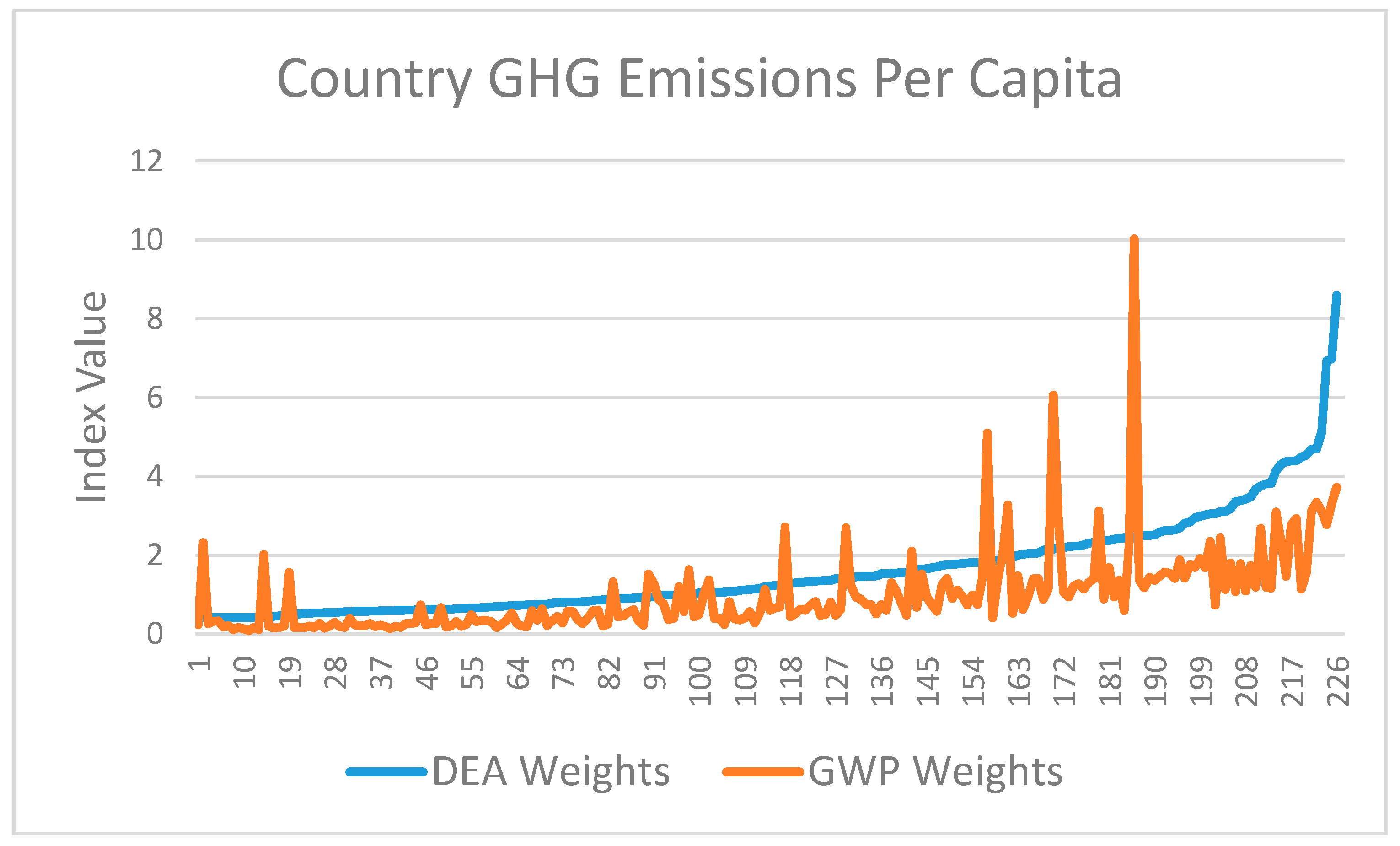
In this exercise, we construct a Composite Greenhouse Gas Index of emissions per capita based on DEA weights and compare it with a Total Greenhouse Gas Index of emissions per capita based on GWP weights. The sample size is 226. The two indices, each normalised by its mean value and ordered in ascending value of the Composite Index, appear in Figure 2.
The two series behave similarly, with correlation coefficient = 0.598 and rank correlation coefficient = 0.820. Both series exhibit a generally declining trend through time, although this is not visible in Figure 2. There is general agreement on the identity of the 25 country-year observations with the highest emissions per capita, but not on the identity of those with the lowest emissions per capita. A large variation in the values of both indices remains, even after controlling for country population; Uganda, India and the U.S. have Composite Index values anywhere from 4 to 8 times those of country-year observations with the lowest values, and Total Index values triple the country-year observations with the lowest values. The Democratic Republic of Congo, which emits suspiciously high amounts of the F gases, is responsible for most of the spikes in the Total Index. The three countries responsible for the largest greenhouse gas emissions in 2010, China, India and the U.S., rank far apart at #44, #103 and #217 respectively in the Composite Index of greenhouse gas emissions per capita.
Turning to weights, we first test the hypotheses that the weights for CH4, N2O and the F gases equal the weight for CO2, which is implicit in the construction of CO2-equivalent gas indices. All three hypotheses are strongly rejected, at confidence levels 0.975, 0.99 and 0.90, respectively. Next, we restrict the sample to the 96 observations attaching a positive weight to CO2, and we test the (equivalent) hypotheses that the ratios of the weights for CH4, N2O and the F gases relative to the weight for CO2 are equal to unity, which also is implicit in the construction of CO2-equivalent gas indices. Again all three hypotheses are strongly rejected, at confidence levels 0.99, 0.99 and 0.975. Finally we test the hypotheses that trade-offs are constants, as GWP weighting imposes. We reject this hypothesis as well, with all three standard deviations exceeding their means by a factor of 1.5 or larger. We conclude that (1) trade-offs are not equal, but vary through time and across countries; and (2) trade-offs are not constant, both of which are implicit under GWP weighting. Moreover, the magnitudes of the weight means suggest that CH4, N2O and the F gases all should have higher weights than their current values of 21, 310 and 1. These results are consistent with our world findings for CH4 and N2O, although they are not comparable for the F gases.
5.2.2. Emissions Per GDP
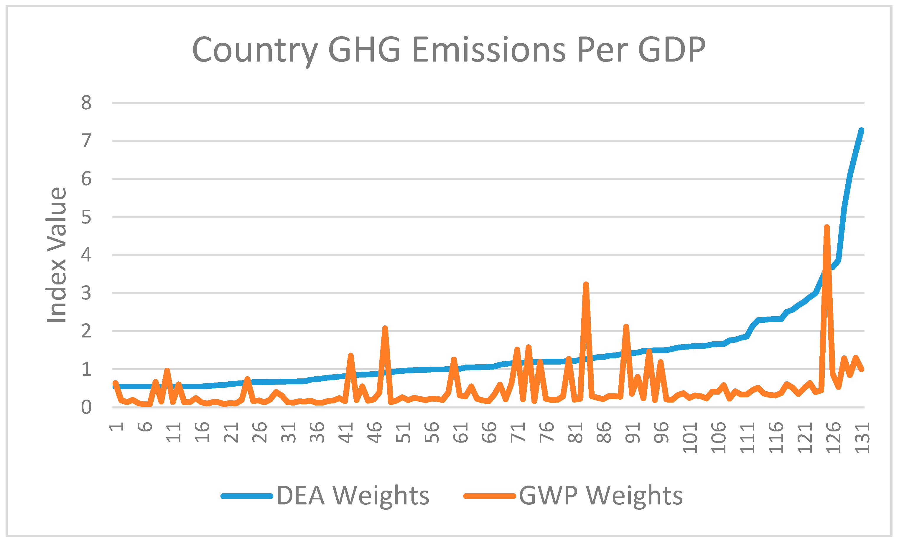
In this exercise, we construct a Composite Greenhouse Gas Index of emissions per GDP based on DEA weights and compare it with a Total Greenhouse Gas Index of emissions per GDP based on GWP weights. We have eliminated six outliers, reducing the sample size from 137 to 131. The six are the Democratic Republic of Congo in 1990, 2000, 2010, Mozambique in 2000, 2010 and Myanmar in 1990; all emitted suspiciously high levels of F gases, ten or more times the sample mean, and all assigned zero shadow values to F gases/GDP. The two indices, each normalised by its mean value and ordered in ascending value of the Composite Index, appear in Figure 3.
The two emissions per GDP indices behave similarly, although the correlation coefficient = 0.340 and the rank correlation coefficient = 0.575 are substantially lower than when emissions are normalised by population. Both series continue to exhibit a generally declining trend through time. Again there is general agreement on the identity of the 25 country-year observations with the highest emissions per GDP, but not on the identity of those with the lowest emissions per GDP. The three countries responsible for the largest greenhouse gas emissions in 2010, China, India and the U.S., rank far apart at #111, #77 and #74 respectively in the per GDP Composite Index, which is the reverse in their ordering when emissions are normalised by population, reflecting China’s and India’s much larger populations and the U.S.’s larger GDP.
The weights and trade-offs findings mirror those when emissions are normalised by population. We reject the hypotheses that the weights for CH4 and the F gases are equal to the weight for CO2 at significance levels of 0.975 and 0.99, but we cannot reject the hypothesis that the weight for N2O is equal to the weight for CO2 at a reasonable significance level. When we restrict the sample to observations having a positive weight for CO2 and test the hypotheses that the three weight ratios, or trade-offs, are equal to unity, we strongly reject all three hypotheses, at significance levels of 0.95, 0.90 and 0.99. We also reject the constant trade-offs hypotheses, with standard deviations exceeding means by factors of three or more. We reach the same conclusions as when emissions are normalised by population: (i) weights are not equal; and (ii) trade-offs are not constant. Both findings run counter to constancy of GWPs. Moreover, the magnitudes of the trade-offs continue to suggest that CH4, N2O and the F gases all should have higher weights than their GWP values.
6. Conclusions and Suggestions for Further Research
The IPCC has developed fixed weights, GWPs, to aggregate individual greenhouse gases into a Total Greenhouse Gas Index. The Paris Agreement uses this index to set emissions reduction targets sufficiently stringent to restrain global warming this century to 2 °C above pre-industrial levels. The GWPs define constant trade-offs between pairs of gases that allow countries to meet their targets in a variety of ways.
The literature surrounding GWPs has criticised their fixity, and the IPCC has updated them as climate science has developed, but they remain stubbornly constant. GWPs remain an integral component of an international policy aimed at constraining greenhouse gas emissions, thereby limiting global warming. The crux of the criticism of the current GWP-based policy is not that it cannot achieve its objective, but rather that it is an inefficient way of pursuing its objective. An efficient approach must incorporate the fact that emissions restrictions impose economic costs on countries, that these costs may vary, across gases, across countries, and through time, and that an efficient abatement policy exploits this variation.
A variety of dynamic optimisation models have been proposed to form the basis of a more efficient policy designed to limit global warming. A central feature of these models is that trade-offs between pairs of gases are generated endogenously, within the models, rather than exogenously by climate scientists. These trade-offs, being endogenous variables, vary across countries and through time, and generate greenhouse gas emissions patterns that differ from those generated from a model based on fixed GWPs. A second feature of these dynamic programming models is their complexity. In contrast, the program developed here offers a relatively simple formulation of an efficient, economic approach to assessing trade-offs between pairs of greenhouse gases across countries and through time. Our formulation retains the natural science component of GWPs, but we provide an overlay through means of endogenous weighting of the economic opportunities for reaching best practice. This formulation has the potential to better allow trade-offs of the gases most suitable for mitigation within each country. This intermediate formulation makes a contribution to the objective of better aligning the physical science understanding of how greenhouse gases heat the climate with the social science understanding that mitigation imposes costs that vary geographically and temporally.
We have conducted three empirical exercises, using data made publicly available by the World Bank. In each exercise we tested two hypothesis. The first hypothesis, constancy of trade-offs between pairs of greenhouse gases, is emphatically rejected in all three exercises, calling into question the value of GWPs for informing efficient policy. However, the second hypothesis, equality of a conventional Total Greenhouse Gas Index based on exogenous GWPs and our Composite Greenhouse Gas Index based on endogenous trade-offs, receives some empirical support, particularly in the world exercise. Our Composite Index increases more slowly, reflecting the efficiency dividend of having the freedom to choose, but the two indices are highly correlated. This finding suggests that similar greenhouse gas emissions patterns can be achieved inefficiently and efficiently, at lower economic cost to emitting countries.
This study can be extended in a number of ways, each using DEA to construct quantity indices of greenhouse gas emissions and endogenous trade-offs.
One exercise, exploiting country data, has four emissions (rather than emissions per capita or per GDP), as variables to be minimised, subject to two “size” constraints, population and GDP. The issue here is, given the size of their population and economy, how well do countries keep their emissions down?
Another exercise, also exploiting country data, would incorporate indicators of country resilience, or adaptability, or of the ability to deal with, perhaps abate, emissions, wherever they originate. For example, population and/or land area with elevation less than five metres (total and % of total) is a vulnerability indicator, while forest area (km2 and % of total) acts as a carbon sink and is a resilience indicator. Additional data are available in the IPCC 2014 Synthesis Report http://www.ipcc.ch/publications_and_data/publications_and_data_reports.shtml and the FAO report http://www.fao.org/docrep/005/ac836e/AC836E03.htm (The 2014 Synthesis Report: Summary for Policymakers has climate impact information on combined land and surface temperature increase, sea level rise, greenhouse gas concentrations, changing precipitation and drought, melting snow and ice, or northern hemisphere snow cover, terrestrial, freshwater and marine species abundance, geographic ranges, and various mitigation and adaptation strategies).
A third exercise, exploiting world data, is inspired by the many scientists who have argued that radiative forcing, although relatively easy to measure, is not a reliable indicator of what we want to measure, namely climate impacts. This suggests an exercise in which greenhouse gas emissions generate climate impacts, and these impacts are measured with a variety of indicators including rising mean surface temperatures, rising sea levels, and extreme weather events.
A final exercise is inspired by the Synthesis Report of the IPCC Fifth Assessment Report, which, as noted previously, identifies four drivers of greenhouse gas emissions. We have used the two most prominent drivers in our empirical exercises, but our assumption of a constant emissions “technology” has ignored changes in the energy intensity of GDP and in the carbon intensity of energy. We view relaxation of the constant “technology” assumption as a potentially significant exercise because technological advances have been responsible for past improvements in both energy efficiency and carbon efficiency, and will continue to be a primary source of future improvements (Google searches on “technology and energy efficiency” and “technology and carbon efficiency” returned approximately 72 million and 95 million results, respectively, testifying to the significance of technology for these two drivers). It is possible to combine these two technology drivers with a third driver, catching up to or falling behind best practice of individual countries, in an effort to quantify the sources of greenhouse gas emissions growth. The Mitigation of Climate Change Report of the IPCC Fifth Assessment Report assists this exercise by providing a detailed analysis of the four drivers and links to relevant databases.
Acknowledgments
All work presented in this article is part of the internal research activity at the Centre for Efficiency and Productivity Analysis in the School of Economics at the University of Queensland, Australia.
Author Contributions
All three authors have made equal contributions to the development of the research question, the analytical methodology, its empirical implementation, and writing the article.
Conflicts of Interest
The authors declare no conflict of interest.
Appendix A
The countries included in the empirical exercise are the 50 largest countries in the World Bank data base (http://data.worldbank.org/indicator) ranked by 2012 population. Twenty-four missing observations reduce the sample size to 226. The fifty countries, ranked by 2012 population, are listed below.
| China | Korea, Rep. |
| India | Tanzania |
| United States | Colombia |
| Indonesia | Spain |
| Brazil | Ukraine |
| Pakistan | Kenya |
| Nigeria | Argentina |
| Bangladesh | Poland |
| Russian Federation | Sudan |
| Japan | Algeria |
| Mexico | Uganda |
| Philippines | Canada |
| Ethiopia | Morocco |
| Vietnam | Iraq |
| Egypt, Arab Rep. | Peru |
| Germany | Venezuela, RB |
| Iran, Islamic Rep. | Uzbekistan |
| Turkey | Afghanistan |
| Congo, Dem. Rep. | Saudi Arabia |
| Thailand | Malaysia |
| France | Nepal |
| United Kingdom | Mozambique |
| Italy | Ghana |
| Myanmar | Yemen, Rep. |
| South Africa | Korea, Dem. People’s Rep. |
References
- Nordhaus, W.D. Economic Growth and Climate: The Carbon Dioxide Problem. Am. Econ. Rev. 1977, 67, 341–346. [Google Scholar]
- Raftery, A.E.; Zimmer, A.; Frierson, D.M.W.; Startz, R.; Liu, P. Less than 2 °C Warming by 2100 Unlikely. Nat. Clim. Chang. 2017, 7, 637–641. [Google Scholar] [CrossRef]
- Schurer, A.P.; Mann, M.E.; Hawkins, E.; Tett, S.F.B.; Hegerl, G.C. Importance of the Pre-Industrial Baseline for Likelihood of Exceeding Paris Goals. Nat. Clim. Chang. 2017, 7, 563–567. [Google Scholar] [CrossRef] [PubMed]
- Fuglestvedt, J.S.; Berngtsen, T.K.; Godal, O.; Skodvin, T. Climate Implications of GWP-based Reductions in Greenhouse Gas Emissions. Geophys. Res. Lett. 2000, 27, 409–412. [Google Scholar] [CrossRef]
- Smith, S.J. The Evaluation of Greenhouse Gases. Clim. Chang. 2003, 58, 261–265. [Google Scholar] [CrossRef]
- Skodvin, T.; Fuglestvedt, J.S. A Comprehensive Approach to Climate Change: Political and Scientific Considerations. Ambio 1997, 26, 351–358. [Google Scholar]
- Reisinger, A.; Ledgard, S.F.; Falconer, S.J. Sensitivity of the Carbon Footprint of New Zealand Milk to Greenhouse Gas Metrics. Ecol. Indic. 2017, 81, 74–82. [Google Scholar] [CrossRef]
- Godal, O. The IPCC’s Assessment of Multidisciplinary Issues: The Case of Greenhouse Gas Indices. Clim. Chang. 2003, 58, 243–249. [Google Scholar] [CrossRef]
- Wigley, T.M.L. The Kyoto Protocol: CO2, CH4, and Climate Implications. Geophys. Res. Lett. 1998, 25, 2585–2588. [Google Scholar] [CrossRef]
- Smith, S.J.; Wigley, T.M.L. Global Warming Potentials: 2. Accuracy. Clim. Chang. 2000, 44, 459–469. [Google Scholar] [CrossRef]
- Lashof, D.A.; Ahuja, D.R. Relative Contributions of Greenhouse Gas Emissions to Global Warming. Nature 1990, 344, 529–531. [Google Scholar] [CrossRef]
- Kandlikar, M. The Relative Role of Trace Gas Emissions in Greenhouse Abatement Policies. Energy Policy 1995, 23, 879–883. [Google Scholar] [CrossRef]
- Shakley, S.; Wynne, B. Global Warming Potentials: Ambiguity or Precision as an Aid to Policy? Clim. Res. 1997, 8, 89–106. [Google Scholar] [CrossRef]
- O’Neill, B.C. The Jury is Still Out on Global Warming Potentials. Clim. Chang. 2000, 44, 427–443. [Google Scholar] [CrossRef]
- Smith, S.J.; Wigley, T.M.L. Global Warming Potentials: 1. Climatic Implications of Emissions Reductions. Clim. Chang. 2000, 44, 445–457. [Google Scholar] [CrossRef]
- Fuglestvedt, J.S.; Bernsten, T.K.; Godal, O.; Sausen, R.; Shine, K.P.; Skodvin, T. Metrics of Climate Change: Assessing Radiative Forcing and Emission Indices. Clim. Chang. 2003, 58, 267–331. [Google Scholar] [CrossRef]
- Lashof, D.A. The Use of Global Warming Potentials in the Kyoto Protocol. Clim. Chang. 2000, 44, 423–425. [Google Scholar] [CrossRef]
- O’Neill, B.C. Economics, Natural Science, and the Costs of Global Warming Potentials. Clim. Chang. 2003, 58, 251–260. [Google Scholar] [CrossRef]
- Shine, K.P. The Global Warming Potential—The Need for an Interdisciplinary Retrial. Clim. Chang. 2009, 96, 467–472. [Google Scholar] [CrossRef]
- Eckhaus, R.S. Comparing the Effects of Greenhouse Gas Emissions on Global Warming. Energy J. 1992, 13, 25–35. [Google Scholar] [CrossRef]
- Schmalensee, R. Comparing Greenhouse Gases for Policy Purposes. Energy J. 1993, 14, 245–255. [Google Scholar] [CrossRef]
- Manne, A.S.; Richels, R.G. An Alternative Approach to Establishing Trade-Offs among Greenhouse Gases. Nature 2001, 410, 675–677. [Google Scholar] [CrossRef] [PubMed]
- Johansson, D.J.A.; Persson, U.M.; Azar, C. The Cost of Using Global Warming Potentials: Analysing the Trade Off between CO2, CH4 and N2O. Clim. Chang. 2006, 77, 291–309. [Google Scholar] [CrossRef]
- Charnes, A.; Cooper, W.W.; Rhodes, E. Measuring the Efficiency of Decision-Making Units. Eur. J. Oper. Res. 1978, 2, 429–444. [Google Scholar] [CrossRef]
- Martín-Gamboa, M.; Iribarren, D. Dynamic Ecocentric Assessment Combining Energy and Data Envelopment Analysis: Application to Wind Farms. Resources 2016, 5, 8. [Google Scholar] [CrossRef]
- Zhou, P.; Ang, B.W.; Poh, K.L. Comparing Aggregating Methods for Constructing the Composite Environmental Index: An Objective Measure. Ecol. Econ. 2006, 59, 305–311. [Google Scholar] [CrossRef]
- Zhou, P.; Delmas, M.A.; Kohli, A. Constructing Meaningful Environmental Indices: A Nonparametric Frontier Approach. J. Environ. Econ. Manag. 2017, 85, 21–34. [Google Scholar] [CrossRef]
- Picazo-Tadeo, A.J.; Castillo-Giménez, J.; Beltrán-Esteve, M. An Intertemporal Approach to Measuring Environmental Performance with Directional Distance Functions: Greenhouse Gas Emissions in the European Union. Ecol. Econ. 2014, 100, 173–182. [Google Scholar] [CrossRef]
- Millington, H.K.; Lovell, J.E.; Lovell, C.A.K. A Framework for Guiding the Management of Urban Stream Health. Ecol. Econ. 2015, 109, 222–233. [Google Scholar] [CrossRef]
- Lovell, C.A.K.; Pastor, J.T. Radial DEA Models without Inputs or without Outputs. Eur. J. Oper. Res. 1999, 118, 46–51. [Google Scholar] [CrossRef]
- Balk, B.M. Price and Quantity Index Numbers: Models for Measuring Aggregate Change and Difference; Cambridge University Press: New York, NY, USA, 2008. [Google Scholar]
- Ebert, U.; Welsch, H. Meaningful Environmental Indices: A Social Choice Approach. J. Environ. Econ. Manag. 2004, 47, 270–283. [Google Scholar] [CrossRef]
- Tone, K. A Slacks-Based Measure of Efficiency in Data Envelopment Analysis. Eur. J. Oper. Res. 2001, 130, 498–509. [Google Scholar] [CrossRef]
- Bradford, D.F. Time, Money and Tradeoffs. Nature 2001, 410, 649–650. [Google Scholar] [CrossRef] [PubMed]
Figure 1.
World Greenhouse Gas Emissions Indices.
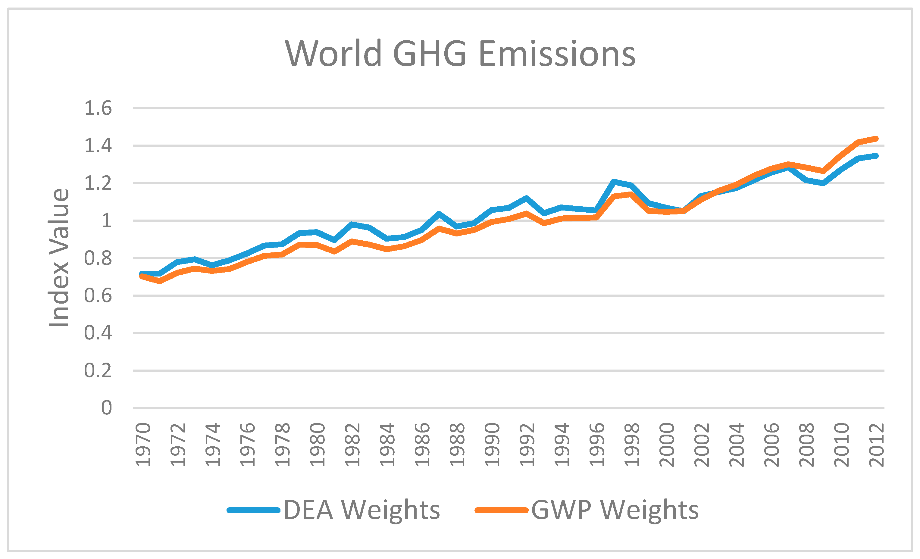
Figure 2.
Country Greenhouse Gas Emissions Per Capita Indices.

Figure 3.
Country Greenhouse Gas Emissions per GDP Indices.


Table 1.
World and Country Greenhouse Gas Emissions Data Sets.
| World Data, 1970–2012 | ||
| Indicator | Label | Units |
| CO2 emissions | CO2 | kt |
| CH4 emissions | CH4 | kt of CO2 equivalent |
| N2O emissions | N2O | kt of CO2 equivalent |
| F gas emissions (HFC + PFC + SF6) | F | kt of CO2 equivalent |
| Country Data, 50 Most Populous Countries, 1970, 1980, 1990, 2000, 2010 | ||
| Indicator | Label | Units |
| CO2 emissions per capita | CO2/P | kt |
| CH4 emissions per capita | CH4/P | kt of CO2 equivalent |
| N2O emissions per capita | N2O/P | kt of CO2 equivalent |
| F gas emissions per capita | F/P | kt of CO2 equivalent |
| Country Data, 50 Most Populous Countries, 1990, 2000, 2010 | ||
| Indicator | Label | Units |
| CO2 emissions per GDP | CO2/GDP | kt |
| CH4 emissions per GDP | CH4/GDP | kt of CO2 equivalent |
| N2O emissions per GDP | N2O/GDP | kt of CO2 equivalent |
| F gas emissions per GDP | F/GDP | kt of CO2 equivalent |
Table 2.
DEA Programs.
| Envelopment Program | Multiplier Program |
|---|---|
| Max | |
| Subject to | Subject to |
| free |
© 2017 by the authors. Licensee MDPI, Basel, Switzerland. This article is an open access article distributed under the terms and conditions of the Creative Commons Attribution (CC BY) license (http://creativecommons.org/licenses/by/4.0/).
Share and Cite
MDPI and ACS Style
Edmonds, H.K.; Lovell, J.E.; Lovell, C.A.K. A New Composite Index for Greenhouse Gases: Climate Science Meets Social Science. Resources 2017, 6, 62. https://doi.org/10.3390/resources6040062
AMA Style
Edmonds HK, Lovell JE, Lovell CAK. A New Composite Index for Greenhouse Gases: Climate Science Meets Social Science. Resources. 2017; 6(4):62. https://doi.org/10.3390/resources6040062
Chicago/Turabian StyleEdmonds, Heidi K., Julie E. Lovell, and C. A. Knox Lovell. 2017. "A New Composite Index for Greenhouse Gases: Climate Science Meets Social Science" Resources 6, no. 4: 62. https://doi.org/10.3390/resources6040062
Note that from the first issue of 2016, this journal uses article numbers instead of page numbers. See further details here.