Groundwater Storage Change Estimation Using Combination of Hydrogeophysical and Groundwater Table Fluctuation Methods in Hard Rock Aquifers

 , and
, and
Abstract
:1. Introduction
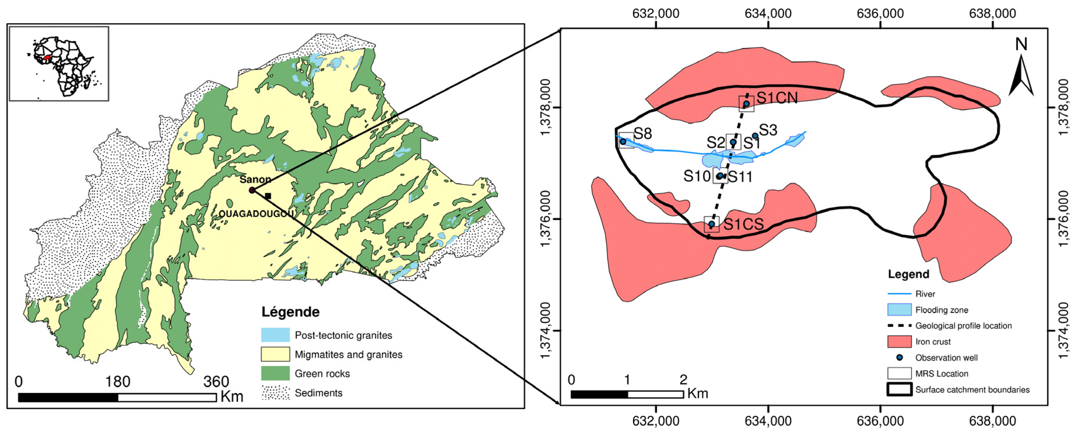
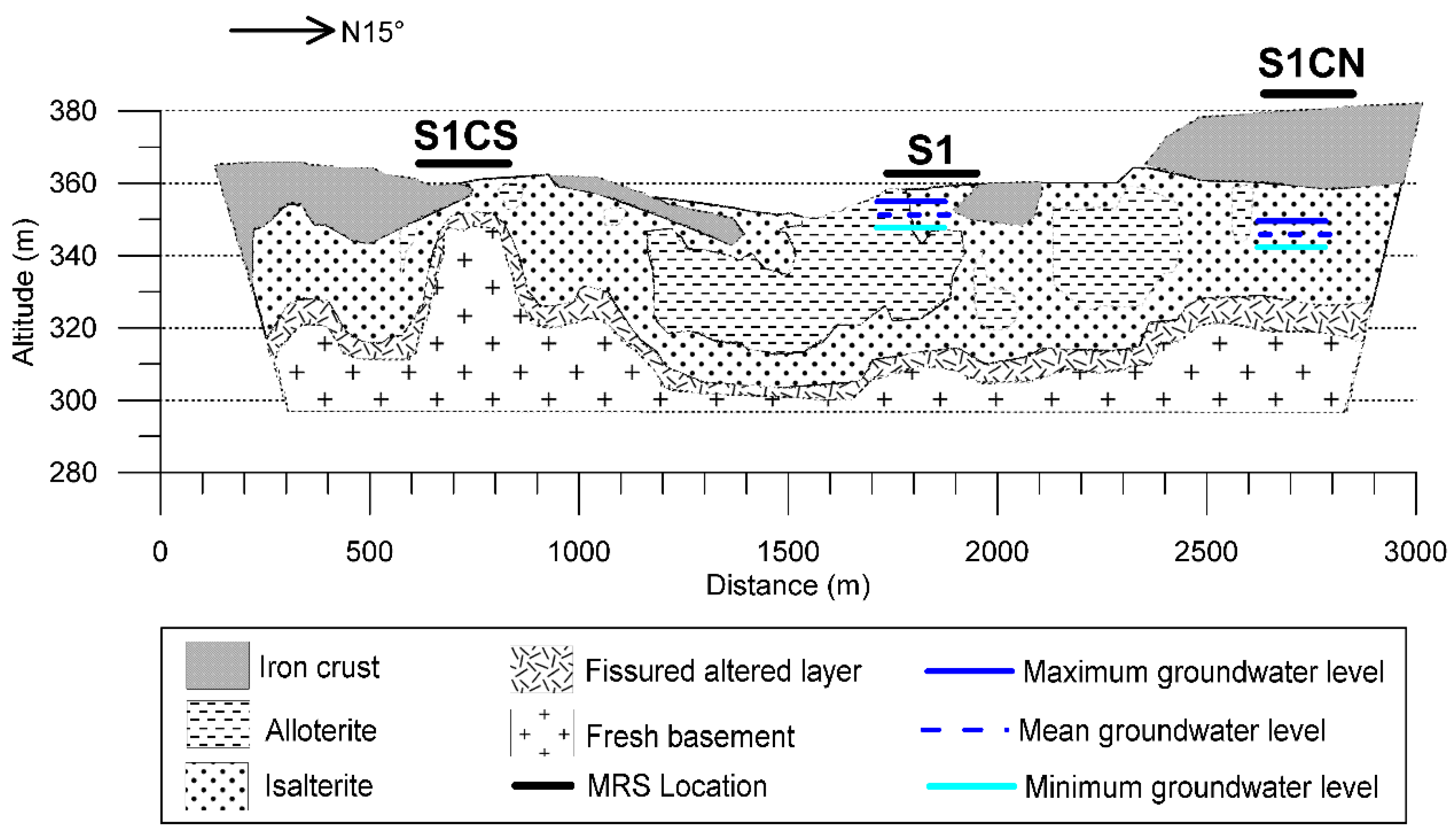
2. Study Site
3. Materials and Methods
3.1. MRS Implementation
- -
- The initial amplitude of the signal E0 which is directly related to the number of hydrogen nuclei that participated to signal response and consequently to the quantity of groundwater;
- -
- The decay parameter T2* is related to the mean size of the pores containing water and therefore to a porosity;
- -
- The phase difference between the signal response and the primary current is related to the electrical resistivity of the reservoir.
3.2. MRS Data Processing
3.3. Estimation of Groundwater Storage Change
3.3.1. Specific Yield Sy
3.3.2. Estimation of Water Table Fluctuation Δh
4. Results and Discussion
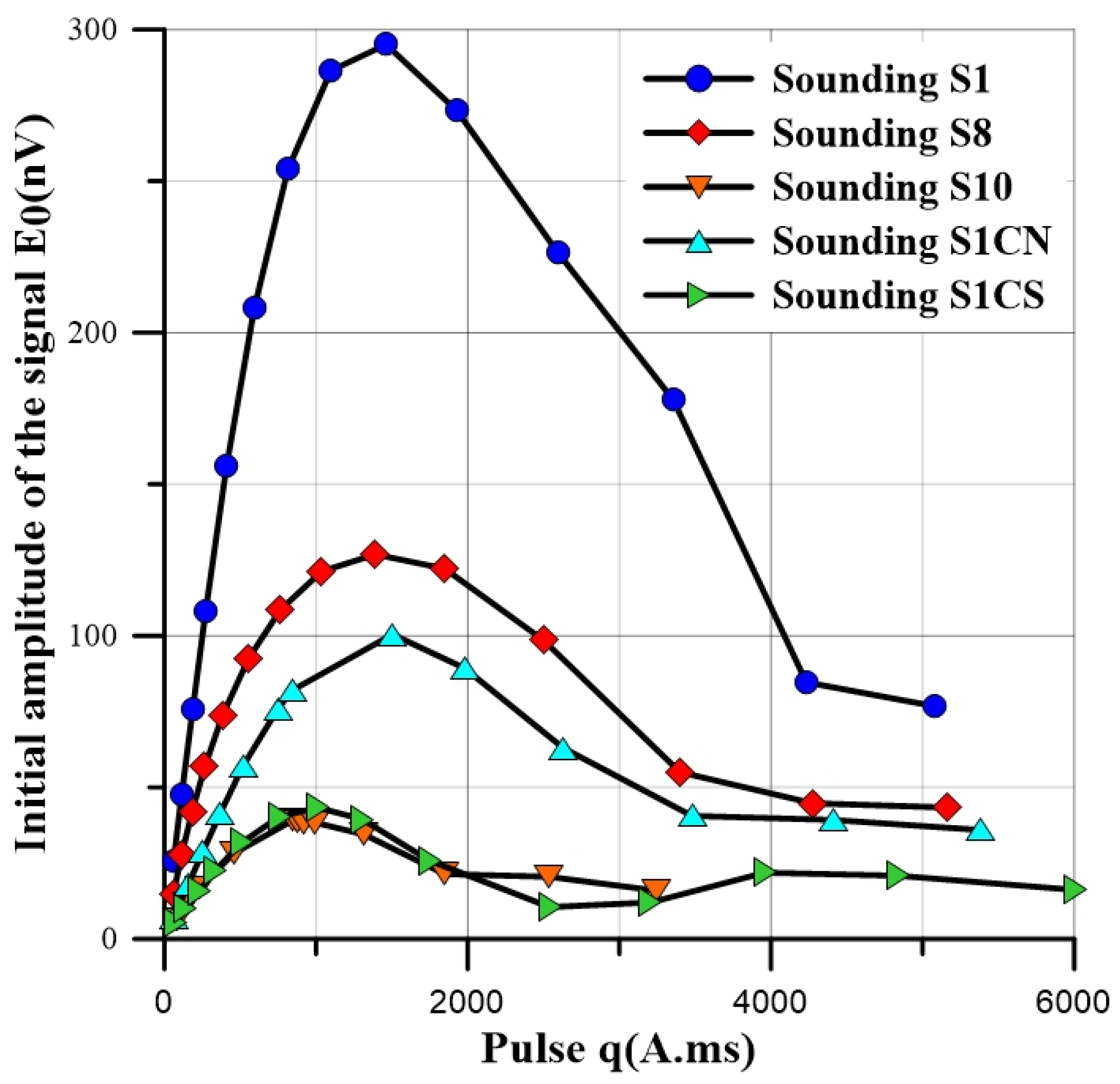
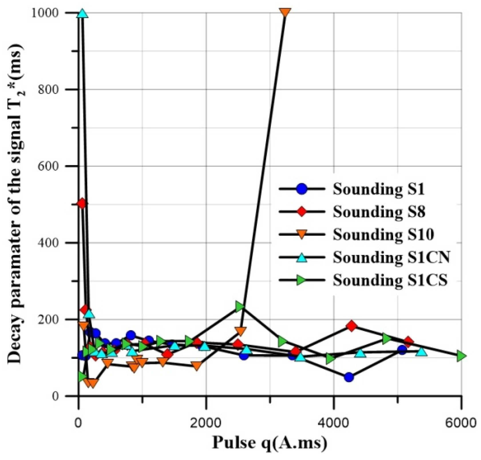
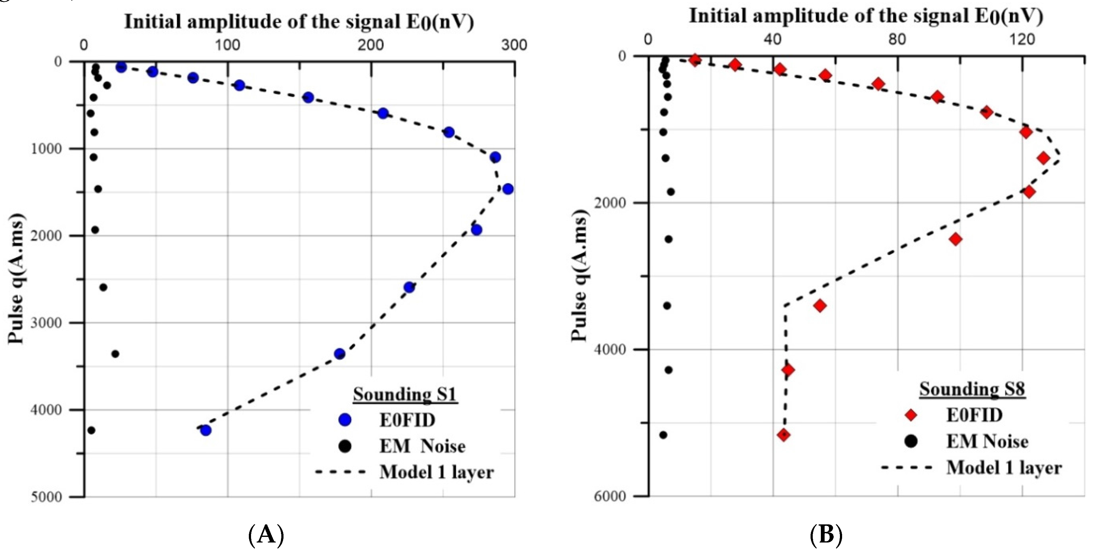
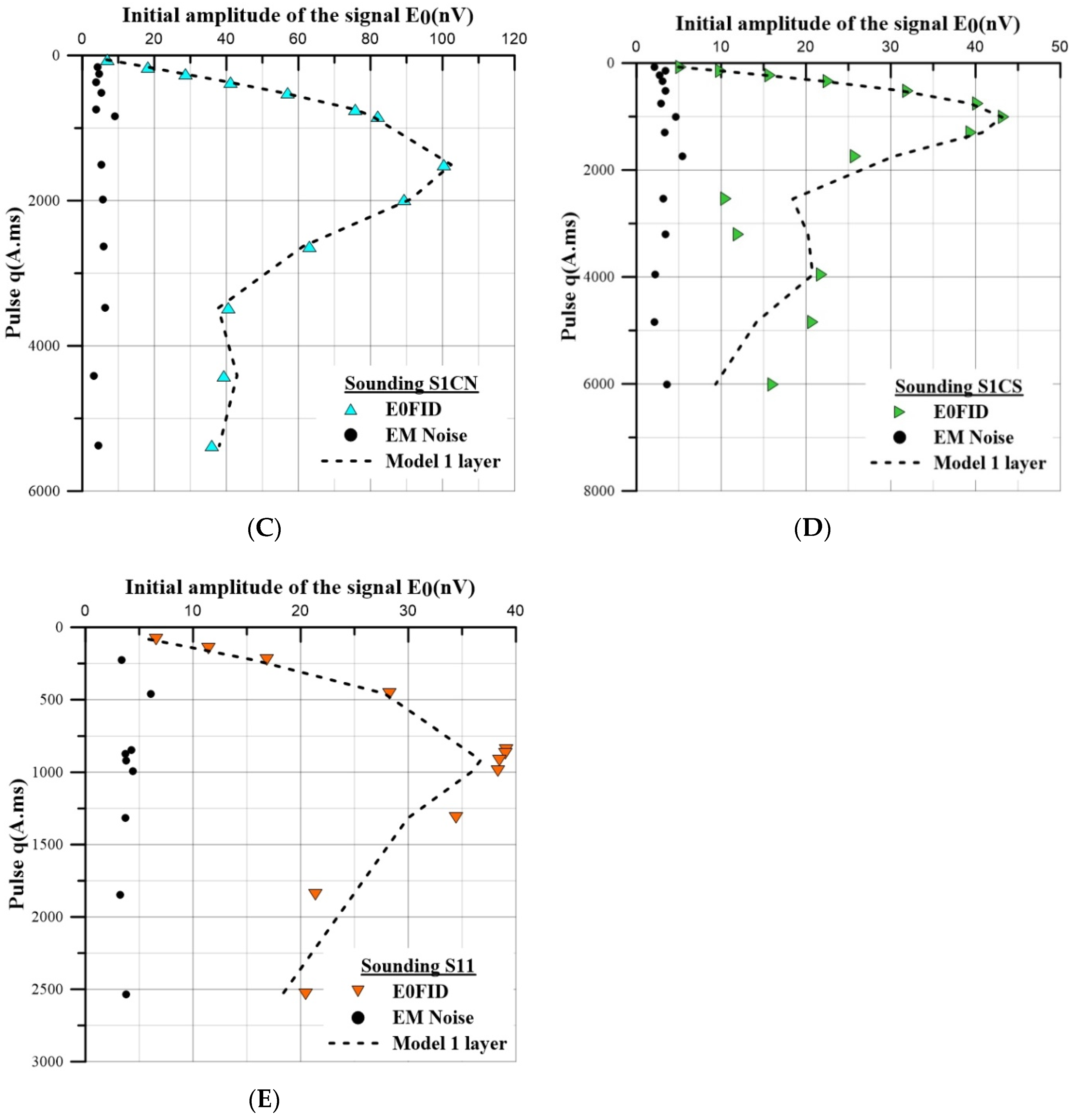
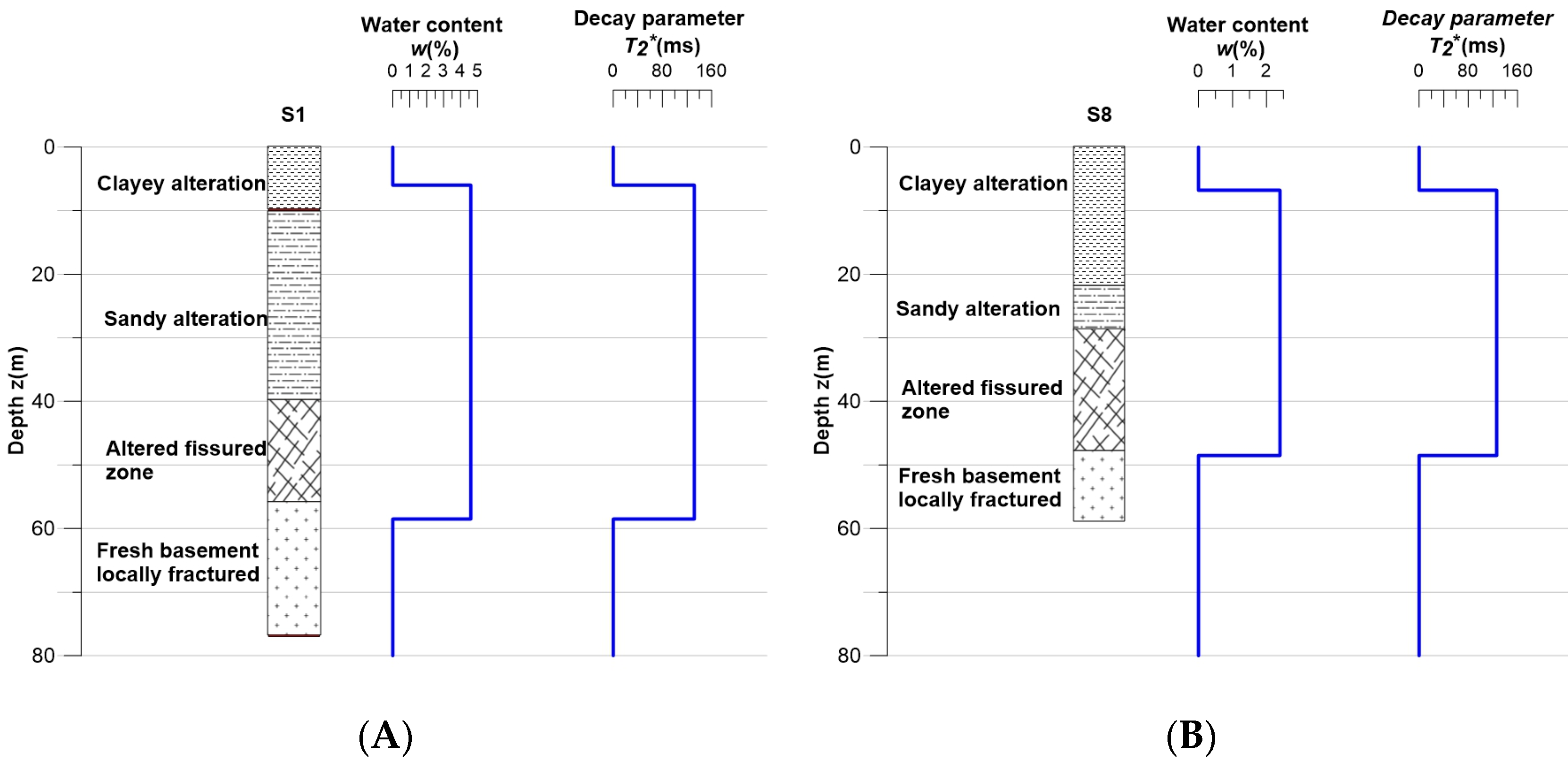
4.1. Distribution of MRS Water Content (WMRS) and Signal Time Decay
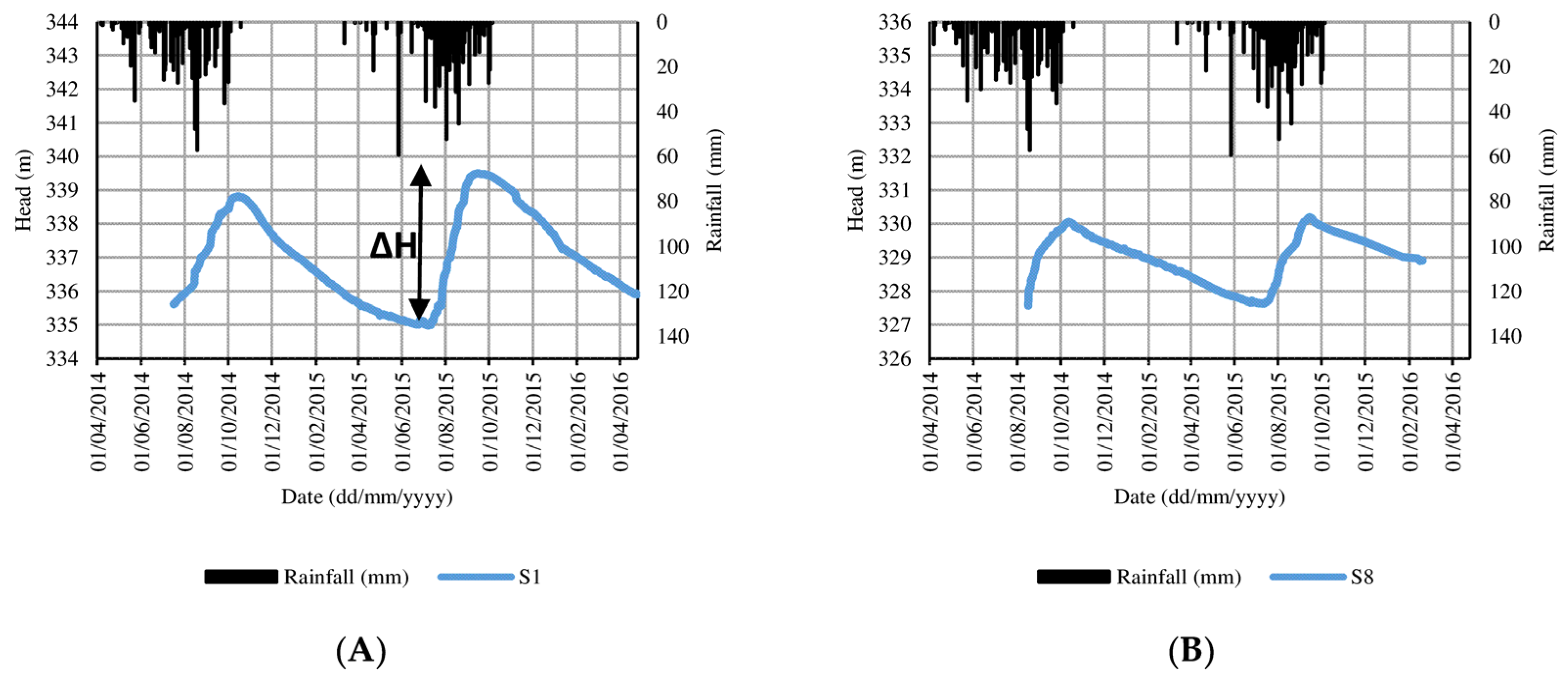
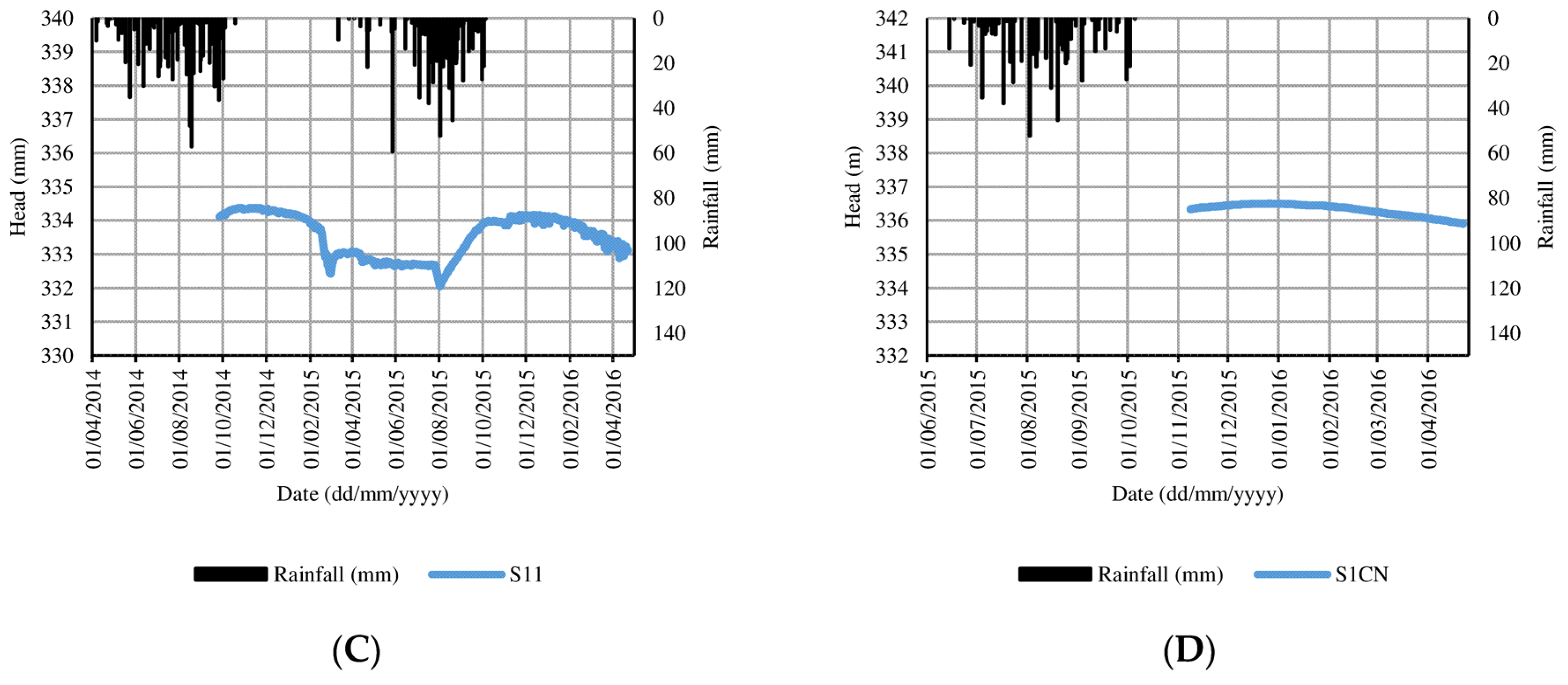
4.2. Water Level Fluctuation
4.3. Change of Groundwater Storage
5. Conclusions
Acknowledgments
Author Contributions
Conflicts of Interest
References
- Giordano, M. Agricultural groundwater use and rural livelihoods in sub-saharan Africa: A first cut assessment. Hydrogeol. J. 2006, 14, 310–318. [Google Scholar] [CrossRef]
- Taylor, R.G.; Kouassi, A.D.; Tindimugaya, C. Groundwater and Climate in Africa—A Review. Hydrol. Sci. J. 2009, 54, 655–664. [Google Scholar] [CrossRef]
- Calow, R.C.; Macdonald, A.M.; Nicol, A.L. Ground water security and drought in Africa: Linking availability, access, and demand. Ground Water 2010, 48, 246–256. [Google Scholar] [CrossRef] [PubMed]
- MacDonald, A.M.; Bonsor, H.C.; Dochartaigh, B.É.Ó.; Taylor, R.G. Quantitative maps of groundwater resources in Africa. Environ. Res. Lett. 2012, 7, 021003. [Google Scholar] [CrossRef]
- Taylor, R.G.; Scanlon, B.; Döll, P.; Rodell, M.; van Beek, R.; Wada, Y.; Longuevergne, L.; Leblanc, M.; Famiglietti, J.S.; Edmunds, M.; et al. Ground water and climate change. Nat. Clim. Chang. 2013, 3, 322–329. [Google Scholar] [CrossRef] [Green Version]
- Yadav, G.S.; Singh, S.K. Integrated resistivity surveys for delineation of fractures for groundwater exploration in hard rock areas. J. Appl. Geophys. 2007, 62, 301–312. [Google Scholar] [CrossRef]
- Döll, P.; Flörke, M. Global-Scale Estimation of Diffuse Groundwater Recharge. Hydrol. Earth Syst. Sci. Discuss. 2007, 4, 4069–4124. [Google Scholar] [CrossRef]
- Howard, K.; Griffith, A. Can the impacts of climate change on groundwater resources be studied without the use of transient models? Hydrol. Sci. J. 2009, 54, 754–764. [Google Scholar] [CrossRef]
- Howard, K.W.; Karundu, J. Constraints on the exploitation of basement aquifers in East Africa—Water balance implications and the role of the regolith. J. Hydrol. 1992, 139, 183–196. [Google Scholar] [CrossRef]
- Scibek, J.; Allen, D.M.; Cannon, A.J.; Whitfield, P.H. Groundwater–surface water interaction under scenarios of climate change using a high-resolution transient groundwater model. J. Hydrol. 2007, 333, 165–181. [Google Scholar] [CrossRef]
- Maréchal, J.C.; Dewandel, B.; Ahmed, S.; Galeazzi, L.; Zaidi, F.K. Combined estimation of specific yield and natural recharge in a semi-arid groundwater basin with irrigated agriculture. J. Hydrol. 2006, 329, 281–293. [Google Scholar] [CrossRef]
- Dewandel, B.; Maréchal, J.C.; Bour, O.; Ladouche, B.; Ahmed, S.; Chandra, S.; Pauwels, H. Upscaling and regionalizing hydraulic conductivity and effective porosity at watershed scale in deeply weathered crystalline aquifers. J. Hydrol. 2012, 416, 83–97. [Google Scholar] [CrossRef]
- Rezaei, A.; Mohammadi, Z. Annual safe groundwater yield in a semiarid basin using combination of water balance equation and water table fluctuation. J. Afr. Earth Sci. 2017, 134, 241–248. [Google Scholar] [CrossRef]
- Dewandel, B.; Caballero, Y.; Perrin, J.; Boisson, A.; Dazin, F.; Ferrant, S.; Chandra, S.; Maréchal, J.-C. A methodology for regionalizing 3-D effective porosity at watershed scale in crystalline aquifers. Hydrol. Process. 2017, 31, 2277–2295. [Google Scholar] [CrossRef]
- Kelly, W.E. Geoelectric sounding for estimating aquifer hydraulic conductivity. Ground Water 1977, 15, 420–425. [Google Scholar] [CrossRef]
- Perdomo, S.; Ainchil, J.E.; Kruse, E. Hydraulic parameters estimation from well logging resistivity and geoelectrical measurements. J. Appl. Geophys. 2014, 105, 50–58. [Google Scholar] [CrossRef]
- Legchenko, A.; Baltassat, J.M.; Beauce, A.; Bernard, J. Nuclear magnetic resonance as a geophysical tool for hydrogeologists. J. Appl. Geophys. 2002, 50, 21–46. [Google Scholar] [CrossRef]
- Vouillamoz, J.M. La Caractérisation des Aquifères par une Méthode non Invasive: Les Sondages par Résonance Magnétique Protonique. Ph.D. Thesis, Université Paris Sud-Paris XI, Orsay, France, 2003. [Google Scholar]
- Vouillamoz, J.M.; Lawson, F.M.A.; Yalo, N.; Descloitres, M. The use of magnetic resonance sounding for quantifying specific yield and transmissivity in hard rock aquifers: The example of Benin. J. Appl. Geophys. 2014, 107, 16–24. [Google Scholar] [CrossRef]
- BRGM-Aquater. Exploitation des Eaux Souterraines en socle Cristallin et Valorisation Agricole: Pilote Expérimental en Milieu Rural Pour les Zones Soudano-Sahéliennes et Sahéliennes; Rapport 33576; BRGM (Bureau de Recherches Géologiques et Minières): Orléans, France, 1991. (In French) [Google Scholar]
- Compaore, G.; Lachassagne, P.; Pointet, T.; Travi, Y. Evaluation du stock d’eau des altérites: Expérimentation sur le site granitique de Sanon (Burkina Faso) Hard Rock Hydrosystems (Proceedings of Rabat Symposium S2, May 1997). IAHSPubI 1997, 241, 37–46. [Google Scholar]
- Soro, D.D.; Koïta, M.; Biaou, C.A.; Outoumbe, E.; Vouillamoz, J.M.; Yacouba, H.; Guérin, R. Geophysical demonstration of the absence of correlation between lineaments and hydrogeologically usefull fractures: Case study of the Sanon hard rock aquifer (central northern Burkina Faso). J. Afr. Earth Sci. 2017, 129, 842–852. [Google Scholar] [CrossRef]
- Dewandel, B.; Lachassagne, P.; Wyns, R.; Maréchal, J.C.; Krishnamurthy, N.S. A generalized 3D geological and hydrogeological conceptual model of granite aquifers controlled by single or multiphase weathering. J. Hydrol. 2006, 330, 260–284. [Google Scholar] [CrossRef]
- Vouillamoz, J.M.; Baltassat, J.M.; Girard, J.F.; Plata, J.; Legchenko, A. Hydrogeological experience in the use of MRS. Bol. Geol. Min. 2007, 118, 385–400. [Google Scholar]
- Legchenko, A.; Valla, P. A review of the basic principles for proton magnetic resonance sounding measurements. J. Appl. Geophys. 2002, 50, 3–19. [Google Scholar] [CrossRef]
- Hoareau, J. Utilisation D’une Approche Couplée Hydrogéophysique Pour L’étude des Aquifères—Applications aux Contextes de Socle et Côtier Sableux. Ph.D. Thesis, Université Joseph Fourier, Grenoble, France, 2009. [Google Scholar]
- Bernard, J. Instruments and field work to measure a Magnetic Rosonance Sounding. Bol. Geol. Min. 2007, 118, 459–472. [Google Scholar]
- Legchenko, A. Magnetic Resonance Imaging for Groundwater; John Wiley & Sons, Inc.: Hoboken, NJ, USA, 2013. [Google Scholar]
- Freeze, R.A.; Cherry, J.A. Groundwater, 1st ed.; Prentice-Hall: Upper Saddle River, NJ, USA, 1979; pp. 36–38. [Google Scholar]
- Chand, R.; Hodlur, G.K.; Prakash, M.R.; Mondal, N.C.; Singh, V.S. Reliable Natural Recharge Estimates in Granitic Terrain. Curr. Sci. 2005, 88, 821–824. [Google Scholar]
- Healy, R.W.; Cook, P.G. Using groundwater levels to estimate recharge. Hydrogeol. J. 2002, 10, 91–109. [Google Scholar] [CrossRef]
- Crosbie, R.S.; Binning, P.; Kalma, J.D. A time series approach to inferring groundwater recharge using the water table fluctuation method. Water Resour. Res. 2005, 41, 1–9. [Google Scholar] [CrossRef]
- Rahi, K.A. Estimating the Hydraulic Parameters of the Arbuckle-Simpson aquifer by Analysis of Naturally-Induced Stresses. Ph.D. Thesis, Oklahoma State University, Stillwater, OK, USA, 2010. [Google Scholar]
- Rahi, K.A.; Halihan, T. Identifying Aquifer Type in Fractured Rock Aquifers using Harmonic Analysis. Ground Water 2013, 51, 76–82. [Google Scholar] [CrossRef] [PubMed]
- Schirov, M.; Legchenko, A.; Créer, G. A new direct non-invasive groundwater detection technology for Australia. Explor. Geophys. 1991, 22, 333–338. [Google Scholar] [CrossRef]
- Descloitres, M.; Seguis, L.; Wubda, M. Caractérisation des Aquifères sur les Sites Amma Catch au Bénin, Apport de la Résonance Magnétique des Protons. Rapport de mission IRD (23 novembre–10 décembre 2006). 2007. Available online: www.amma-catch.org/IMG/pdf/rapport_rmp_benin_sans_annexes.pdf (accessed on 20 September 2017).
- Boucher, M.; Fraveau, G.; Descloitres, M.; Vouillamoz, J.-M.; Massuel, S.; Nazoumou, Y.; Cappalaere, B.; Legchencko, A. Contribution of geophysical surveys to groundwater modelling of a porous aquifer in semiarid Niger: An overview. C. R. Geosci. 2009, 341, 800–809. [Google Scholar] [CrossRef]
- Ajami, H.; Maddock, T.; Meixner, T.; Hogan, J.F.; Guertin, D.P. RIPGISNET: A GIS Tool for Riparian groundwater evapotranspiration in MODFLOW. Ground Water 2012, 50, 154–158. [Google Scholar] [CrossRef] [PubMed]
- Koïta, M.; Yonli, H.F.; Soro, D.D.; Dara, A.E.; Vouillamoz, J.M. Taking into Account the Role of the Weathering Profile in Determining Hydrodynamic Properties of Hard Rock Aquifers. Geosciences 2017, 7, 89. [Google Scholar] [CrossRef]


| MRS Location | Water Content WMRS (%) | Time Decay T2* (ms) | Aquifer Top (m) | Aquifer Thickness Δz (m) | Water Height wΔz (m) | Ratio Signal/Noise | RMS (nV) |
|---|---|---|---|---|---|---|---|
| S1 | 4.6 | 131.7 | 6 | 52.5 | 2.42 | 9.69 | 8.96 |
| S8 | 2.2 | 126.3 | 6.8 | 41.7 | 1 | 7.17 | 6.42 |
| S10 | 1.3 | 83.7 | 6.8 | 36.2 | 0.47 | 2.29 | 2.24 |
| S1CN | 4.3 | 124.7 | 14.8 | 37.2 | 1.6 | 5.13 | 4.52 |
| S1CS | 1.4 | 132.2 | 8.6 | 41.7 | 0.58 | 3.77 | 5.09 |
| Sites | MRS Water Content (%) | Sy (%) | Δh (m) | ΔS (m) | Rainfall (mm) | ΔS/Rainfall (%) |
|---|---|---|---|---|---|---|
| Central valley (S1) | 4.6 | 2.4 | 4.85 | 0.116 | 843 | 13.7 |
| Outlet (S8) | 2.4 | 1.3 | 2.53 | 0.032 | 843 | 3.7 |
© 2018 by the authors. Licensee MDPI, Basel, Switzerland. This article is an open access article distributed under the terms and conditions of the Creative Commons Attribution (CC BY) license (http://creativecommons.org/licenses/by/4.0/).
Share and Cite
Koïta, M.; Yonli, H.F.; Soro, D.D.; Dara, A.E.; Vouillamoz, J.-M. Groundwater Storage Change Estimation Using Combination of Hydrogeophysical and Groundwater Table Fluctuation Methods in Hard Rock Aquifers. Resources 2018, 7, 5. https://doi.org/10.3390/resources7010005
Koïta M, Yonli HF, Soro DD, Dara AE, Vouillamoz J-M. Groundwater Storage Change Estimation Using Combination of Hydrogeophysical and Groundwater Table Fluctuation Methods in Hard Rock Aquifers. Resources. 2018; 7(1):5. https://doi.org/10.3390/resources7010005
Chicago/Turabian StyleKoïta, Mahamadou, Hamma Fabien Yonli, Donissongou Dimitri Soro, Amagana Emmanuel Dara, and Jean-Michel Vouillamoz. 2018. "Groundwater Storage Change Estimation Using Combination of Hydrogeophysical and Groundwater Table Fluctuation Methods in Hard Rock Aquifers" Resources 7, no. 1: 5. https://doi.org/10.3390/resources7010005