On Goodput and Energy Measurements of Network Coding Schemes in the Raspberry Pi

Abstract

Given that next generation networks are expected to be populated by a large number of devices, there is a need for quick deployment and evaluation of alternative mechanisms to cope with the possible generated traffic in large-scale distributed data networks. In this sense, the Raspberry Pi has been a popular network node choice due to its reduced size, processing capabilities, low cost and its support by widely-used operating systems. For information transport, network coding is a new paradigm for fast and reliable data processing in networking and storage systems, which overcomes various limitations of state-of-the-art routing techniques. Therefore, in this work, we provide an in-depth performance evaluation of Random Linear Network Coding (RLNC)-based schemes for the Raspberry Pi Models 1 and 2, by showing the processing speed of the encoding and decoding operations and the corresponding energy consumption. Our results show that, in several scenarios, processing speeds of more than 80 Mbps in the Raspberry Pi Model 1 and 800 Mbps in the Raspberry Pi Model 2 are attainable. Moreover, we show that the processing energy per bit for network coding is below 1 nJ or even an order of magnitude less in these scenarios.

1. Introduction

Due to the advent of the Internet of Things (IoT), approximately 50 billion devices ranging from sensors to phones are expected to be connected through data networks in a relatively short period of time [1]. This massive deployment requires the design and testing of new distributed systems that permit one to manage the amount of traffic from the proposed services provided by these devices. Therefore, development platforms that help to quickly deploy, analyze and evaluate this type of scenario are highly desirable for research. With the emergence of the Raspberry Pi (Raspi), a lrelatively powerful low-cost computer with the size of a credit card, these evaluations are becoming possible now. This platform has been used as general purpose hardware for IoT applications as reported in surveys, such as [2]. In these applications, the Raspi might be the sensoring or computing entity (or even both) for a required task. To achieve this, it can be extended from being a simple computer using self-designed or already available extension modules.

A benefit of using the Raspi as a development platform is its large community of supporters. By running standard operating systems, such as Linux or Windows, this permits one to utilize standard, well-tested and reliable tools to administrate and maintain these networks in a flexible, stable and supported manner, which is a major requirement to make a scalable deployment. Moreover, by enabling system designers to configure and deploy several devices at the same time, possible deployments of tens, hundreds or even thousands of Raspberry Pi’s would allow one to analyze representative data patterns of the IoT. Different use cases of IoT applications employing the Raspi as a building block can be found in the literature. A basic study of the Raspi as a possible device for sensor applications can be found in [3]. The authors in [4] consider using the Raspi as an IPv6 over Low power Wireless Personal Area Networks (6LoWPAN) gateway for a set of sensor and mobile devices to an Internet Protocol (IP) Version 6 network. In [5], a general purpose sensoring platform for IoT is presented using the Raspi as its basic building block. Various interesting IoT use cases are the works presented in [6,7,8,9]. In [6], many Raspis are used as controllable smart devices with network connectivity that may ubiquitously interact with different users, each represented by a mobile device through a smartphone application. The study in [7] considers Raspis as a data processing unit for disseminating artwork content in smart museums. An IoT setting where the Raspi is employed as a nano-server in distributed storage and computing can be found in [8]. Finally, in [9], the authors present the Raspi as the processing entity of an unmanned areal vehicle application to increase the resilience of wireless sensor networks. However, despite all of these advances in the IoT area regarding the exploitation of the Raspi capabilities, the application data are forwarded using former conventional routing methods, which may not satisfy the need of a distributed network for IoT applications as mentioned earlier.

In this context, introduced in [10], Network Coding (NC) constitutes a paradigm shift in the way data networks are understood by changing how information is sent through them and stored at the end devices. Instead of treating the packets as atomic unmodifiable units, packets are seen as algebraic entities in a Galois Field (GF) that can be operated on to create new coded packets. This permits one to remove the limitation of sending specific packets by now sending coded packets as linear equations of the original ones. This change in the way of seeing how the data are represented brings new features that can be exploited. In this way, instead of typically encoding and decoding on a hop basis, relaying nodes can take part in the coding process without needing to decode. Therefore, a relay can recode packets, i.e., encode again previously-received encoded (but not decoded) packets in order to reduce delay and still take advantage of the data representation for the next hop. This new type of coding across the network is proven to achieve the multicast capacity [10,11].

Compared to other broadly-used coding schemes, such as Low Density Parity Check (LDPC) codes [12] or Reed–Solomon codes [13], network coding is a technology that has been studied and implemented in real systems since the early years of its conception. A decentralized network code that has been proven to achieve the multicast capacity with very high probability is RLNC [14]. Later, a work observing the benefits of employing RLNC in meshed networks is the Multi-path Opportunistic Routing Engine (MORE) protocol addressed in [15]. Shortly afterwards, the authors in [16] showed the performance of an implementation of the COPE protocol for the two-way relay channel in a wireless network, which relied on minimalistic coding and obtaining gains over a forwarding scheme. Later, the work in [17] used commercially-available Symbian OS mobile phones to implement network coding in a Device to Device (D2D) cooperation-based application. Furthermore, in [18], the Kodo library was introduced. Kodo is a C++11 network coding library intended to make network coding basic functionalities easily available for both the research community and commercial entities. Based on Kodo, the Coding Applied To Wireless On Mobile Ad-hoc Networks (CATWOMAN) protocol [19] is implemented on top of the Better Approach To Mobile Ad-hoc Networking (BATMAN) protocol [20] for WiFi multi-hop meshed networks. It uses some of the intuition from COPE, but it is deployed within the X topology with overhearing links. Its source code is available as open source in the Linux kernel. Moreover, many other successful implementations have been tested on real-world systems, such as found in [21,22,23,24]. For the Raspberry Pi device, an evaluation of RLNC can be found in [25]. However, this evaluation focused particularly on observing the achievable speeds only for RLNC with different configurations of the code parameters. In this previous work, a relevant practical aspect that was not evaluated was the use of hardware acceleration through Single Instruction Multiple Data (SIMD) or the multi-core capabilities of more advanced Raspi models. These features are becoming more frequent in new processors to largely increase their computational power for the upcoming demand. In this sense, the Raspberry Pi posses an Advanced RISC Machine (ARM) architecture that could be multi-core, as mentioned, and also exploits the SIMD feature with the optimized NEON instruction set, but still to the best of our knowledge, there has been no documentation in the literature about these capabilities.

Therefore, in this work, we provide detailed measurements of the goodput (processing speed) and energy consumption of Raspi Models 1 and 2, when performing network coding operations with different codecs based on RLNC such as: full dense RLNC, multi-core enabled RLNC, sparse RLNC and tunable sparse RLNC. For these coding schemes, the encoder and decoder implementations from Kodo are able to detect and make use of the SIMD through the NEON instruction set of the Raspberry Pi by recognizing the ARM architecture with its multicore capabilities. We assess the Raspi performance excluding the effect of packet losses or delays in order to have a description of the processing and energy consumption for only the codes in terms of their parameters. To achieve this, we perform a measurement campaign with the indicated coding schemes and their parameters in various models of a Raspberry Pi device. Our measurements permit us to characterize the mentioned metrics of these devices showing that processing speeds of 800 Mbps and processing energy per bit values of 0.1 nJ are possible. Our work is organized as follows. Section 2 defines the coding schemes employed in our study. Later, in Section 3, we describe the considered metrics and methodology for the performance comparison of the codes deployed in the Raspi. In Section 4, we show the measurements in the Raspi models of the mentioned metrics providing full discussions about the observed operational regimes and effects. Final conclusions and future work are reviewed in Section 5.

2. Coding Schemes

In this section, we present the considered coding schemes that are evaluated in the Raspi 1 and 2. We introduce a definition for the primitive coding operations, e.g., encoding, decoding and recoding (where it applies) for each coding scheme. Later, we address particular schemes, which are obtained by modifying the basic coding operations that provide better processing speeds, which is particularly relevant for the Raspi. Finally, we include a review of algorithms for network coding that exploit the multicore capabilities of the Raspi 2.

2.1. Random Linear Network Coding

RLNC is an example of intra-session NC, i.e., data symbols from a single flow are combined with each other. In this type of network coding, g original data packets, also called a generation [26], $P_j,j\in [1,2,\dots ,g]$, each of B bytes, are used to create coded packets using random linear combinations of the original ones. In the following subsections, we describe the basic functionalities of RLNC.

2.1.1. Encoding

In RLNC, any coded packet is a linear combination of all of the original packets. For the coding scheme, packets are seen as algebraic entities formed as a sequence of elements from $GF\left(q\right)$, which is a GF of size q. Later, each original packet is multiplied by a coding coefficient from $GF\left(q\right)$. The coding coefficients are chosen uniformly at random from the GF by the encoder. To perform the multiplication of a packet by a coding coefficient, the coefficient is multiplied for each of the elements in the concatenation that composes an original packet, preserving the concatenation. Later, all resulting packets are added within the GF arithmetics together to generate a coded packet. Thus, a coded packet can be written as:

$$\begin{array}{cc}\hfill C_i& =\underset{j=1}{\overset{g}{⨁}}{v}_{ij}\otimes P_j,\forall i\in [1,2,\dots )\hfill \end{array}$$

(1)

In (1), $C_i$ is the generic coded packet. In principle, the encoder may produce any number of coded packets, but a finite number is produced in practice given that a decoder needs only g linearly-independent coded packets to decode the batch. Furthermore, in (1), $v_{ij}$ is the coding coefficient used in the i-th coded packet and assigned to multiply the j-th original packet.

For indicating to a receiver how the packets were combined to create a coded one, a simple, yet versatile choice is to append its coding coefficients as a header in the coded packet. Hence, an amount of overhead is included in every coded packet given that we need to provide some signaling needed for decoding. The coding coefficients overhead amount for packet i, $|v_i|$, can be quantified as:

$$\begin{array}{cc}\hfill |v_i|& =\sum _{j=1}^g\left|v_{ij}\right|=g\times \lceil {log}_2\left(q\right)\rceil \left[\mathrm{bits}\right].\hfill \end{array}$$

(2)

2.1.2. Decoding

To be able to decode a batch of g packets, a linearly-independent set of g coded packets, $C_i,i\in [1,2,\dots ,g]$, is required at a decoder. Once this set has been collected for a decoder, the original packets can be found by computing the solution of a system of linear equations using GF arithmetics. Thus, we define $\mathbf{C}={\left[C_1\dots C_g\right]}^T$, $\mathbf{P}={\left[P_1\dots P_g\right]}^T$ and the coding matrix $\mathbf{V}$ that collects the coding coefficients for each of the g coded packets, as follows:

$$\begin{array}{c}\hfill \mathbf{V}=\left[\begin{array}{c}\underset{―}{v_1}\\ ⋮\\ \overline{v_g}\end{array}\right]=\left[\begin{array}{ccc}{v}_{11}& \dots & v_{1g}\\ ⋮& \ddots & ⋮\\ v_{g1}& \dots & v_{gg}\end{array}\right].\end{array}$$

(3)

Algebraically, decoding simplifies to finding the inverse of $\mathbf{V}$ in the linear system $\mathbf{C}=\mathbf{V}\mathbf{P}$, which can be achieved using efficient Gaussian elimination techniques [27]. On real applications, decoding is performed on-the-fly, e.g., the pivots are computed as packets are progressively received, in order to minimize the computation delay for each step.

A decoder starts to calculate and subtract contributions from each of the pivot elements, e.g., leftmost elements in the main diagonal of (3), from top to bottom. The purpose is to obtain the equivalence $\mathbf{V}$ in its reduced echelon form. The steps for reducing the matrix by elementary row operations are carried out each time a linearly-independent packet is received. Once in reduced echelon form, packets can be retrieved by doing a substitution starting from the latest coded packet. In this way, the amount of elementary operations at the end of the decoding process is diminished.

2.1.3. Recoding

As an inherent property of RLNC, an intermediate node in the network is able to create new coded packets without needing to decode previously-received packets from an encoding source. Therefore, RLNC is an end-to-end coding scheme that permits one to recode former coded packets at any point in the network without requiring a local decoding of the data. In principle, a recoded packet should be indistinguishable from a coded one. Thus, we define a recoded packet as $R_i$ and consider the coding coefficients $w_{i1},\dots ,w_{ig}$ as used to create $R_i$. Later, a recoded packet can be written as:

$$\begin{array}{c}\hfill R_i=\underset{j=1}{\overset{g}{⨁}}{w}_{ij}\otimes C_j,\forall i\in [1,\dots ).\end{array}$$

(4)

In (4), $w_{ij}$ is the coding coefficient used in the i-th recoded packet and assigned to multiply a previously-coded packet $C_j$. These coding coefficients are again uniformly and randomly chosen from $GF\left(q\right)$. However, these $w_{ij}$’s are not appended to the previous coding coefficients. Instead, the system will update the previous coefficients. Due to the linearity of the operation, this update reduces to recombining the coding coefficients equivalent to each original packet with the weight of the $w_{i,j}$.Therefore, we define the local coding matrix $\mathbf{W}$ in the same way as it was made for $\mathbf{V}$. Thus, the local coding matrix can be written as:

$$\begin{array}{c}\hfill \mathbf{W}=\left[\begin{array}{c}\underset{―}{w_1}\\ ⋮\\ \overline{w_g}\end{array}\right]=\left[\begin{array}{ccc}{w}_{11}& \dots & w_{1g}\\ ⋮& \ddots & ⋮\\ w_{g1}& \dots & w_{gg}\end{array}\right].\end{array}$$

(5)

With the definitions from (3) and (5), the recoded packets $\mathbf{R}={\left[R_1\dots R_g\right]}^T$ are written as $\mathbf{R}=\left(\mathbf{W}\mathbf{V}\right)\mathbf{P}$. Here, we recognize the relationship between original and recoded packets. The resulting coding matrix is the multiplication of matrices $\mathbf{W}$ and $\mathbf{V}$. Denoting ${\left(\mathbf{W}\mathbf{V}\right)}_{ij}$ as the element in the i-th row and j-th column of $\left(\mathbf{W}\mathbf{V}\right)$, this term is the resulting coding coefficient used to create $R_i$ after encoding the original packet $P_j$ recoding it locally in an intermediate node. Finally, the appended coefficients for $R_i$ are ${\left(\mathbf{W}\mathbf{V}\right)}_{ik}$ with $k\in [1,2,\dots ,g]$. By doing some algebra, each ${\left(\mathbf{W}\mathbf{V}\right)}_{ij}$ term can be verified to be computed as:

$$\begin{array}{c}\hfill {\left(\mathbf{W}\mathbf{V}\right)}_{ij}=\sum _{k=1}^g{w}_{ik}{v}_{kj},\forall i,j\in [1,2,\dots ,g]\times [1,2,\dots ,g].\end{array}$$

(6)

This update procedure on the coding coefficients is carried by all of the recoders in a given network, therefore allowing any decoder to compute the original data after Gaussian elimination, regardless of the amount of times recoding was performed and without incurring in any additional overhead cost for signaling. Similar to the encoding operation, any decoder that collects a set of g linearly-independent recoded packets with their respective coefficients will be able to decode the data as mentioned before in Section 2.1.2.

2.2. Sparse Random Linear Network Coding

In Sparse Random Linear Network Coding (SRLNC), instead of considering all of the packets to create a coded packet as in RLNC, an encoder sets more coding coefficients to zero when generating a coded packet with the purpose of reducing the overall processing. Decoding is the same as in RLNC, but given that the coding matrices are now sparse means that there will be less operations to perform in the decoding process. Recoding, although theoretically possible, is omitted since it requires the use of heuristics to keep packets sparse after recoding, which is inherently sub-optimal. In what follows, we describe the coding scheme with two different methods to produce sparse coded packets.

2.2.1. Method 1: Fixing the Coding Density

A way to control the amount of non-zero coding coefficients is to set a fixed ratio of non-zero coefficients in the encoding vector of size g. We refer to this fixed ratio as the average coding density d. Thus, for any coded packet $C_i$ with coding coefficients $v_{ij},j\in [1,2,\dots ,g]$, its coding density is defined as follows:

$$\begin{array}{c}\hfill d=\frac{{\sum }_{j=1}^{g}f\left(v_{ij}\right)}{g},f\left(v_{ij}\right)=\left\{\begin{array}{cc}0\hfill & ,v_{ij}=0\hfill \\ 1\hfill & ,v_{ij}\ne 0\hfill \end{array}\right.\end{array}$$

(7)

From the density definition in (7), it can be observed that $0\le d\le 1$. As g increased, we obtain more granularity in the density. Notice that the special case of $d=0$ has no practical purpose, since it implies just zero padded data. Therefore, a practical range for the density excludes the zero case, $0<d\le 1$. Furthermore, in $GF\left(2\right)$, there is no benefit of using $d>0.5$ in terms of generating linearly-independent packets [28]. Thus, we limit the range to $0<d\le 0.5$ in $GF\left(2\right)$.

To achieve a desired average coding density in the coefficients, for each of them, we utilize a set of Bernoulli random variables all with parameter d as its success probability, i.e., ${\mathbb{B}}_j\sim Bernoulli\left(d\right),\forall j\in [1,2,\dots ,g]$. In this way, we can represent a coded packet in SRLNC as:

$$\begin{array}{cc}\hfill C_i& =\underset{j=1}{\overset{g}{⨁}}{\mathbb{B}}_j{v}_{ij}\otimes P_j,v_{ij}\ne 0\forall i\in [1,\dots ),d\in \left\{\begin{array}{cc}(0,0.5]\hfill & ,q=2\hfill \\ (0,1]\hfill & ,q>2\hfill \end{array}\right.\hfill \end{array}$$

(8)

In (8), we have the requirement for the coding coefficient to not be zero, since we want to ensure that a coding coefficient is generated for any random trial, where ${\mathbb{B}}_j=1$. Therefore, in our implementation of SRLNC, we exclude the zero element and then pick uniformly-distributed random elements from $GF\left(q\right)-\left\{0\right\}$. Furthermore, we have specified a dependency on the field size for practical density values. In the case of employing $GF\left(2\right)$, the maximum plausible density is restricted up to 0.5, since higher values incur in more frequent linearly-dependent coded packets [28] accompanied by higher coding complexity.

Reducing d enables the encoder to decrease the average number of packets mixed to make a coded one. This reduces the complexity of the encoder since it needs to mix less packets. Moreover, it also simplifies the decoder processing given that less nonzero coding coefficients are required to be operated during the Gaussian elimination stage.

The drawback of this scheme is that coded packets from the encoder become more linearly dependent on each other as the density is reduced. This leads to transmission overhead since another coded packet is required to be sent for every reception of a redundant packet. Furthermore, this method may still generate a coded packet, which does not contain any information. For example, we might find the case where $\left[{\mathbb{B}}_1,\dots ,{\mathbb{B}}_g\right]=\mathbf{0}$ to occur frequently for low densities. In that case, the encoder discards the coded packet and tries to generate a new one to avoid the negative impact on overall system performance.

2.2.2. Method 2: Sampling the Amount of Packets to Combine

The method described from (8) results in a fast implementation in terms of execution time for $d\ge 0.3$ [29]. It is however not able to utilize the full performance potential for low densities, as the total number of Bernoulli trials remains unchanged independently of the density. Thus, we introduce a second method that permits a faster implementation for low coding densities [29].

For this method, we first obtain the amount of packets that we will combine to create a coded packet. To do so, a random number, $\mathbb{M}$, of the original packets is used to produce a coded packet. For our case, $\mathbb{M}$ is binomially distributed with parameters g for the number of trials and d for its success probability, e.g., $\mathbb{M}\sim Binomial(g,d)$. However, when sampling from this distribution, the case $\mathbb{M}=0$ occurs with a non-zero probability. In order to handle this special case, our implementation considers $\mathbb{K}=max(1,\mathbb{M})$ as the final amount of packets to be mixed together. In this way, we always ensure that at least one packet is encoded.

The only caveat is that the case of $\mathbb{K}=1$ occurs slightly more often than $\mathbb{M}=1$ in the original distribution, but for the considered density range in this method, this is not a significant modification [29]. Then, once the distribution for the number of packets to mix has been defined, we sample a value m from $\mathbb{M}$ and compute $k=max(1,m)$. Later, we create a set $\mathcal{K}$ with cardinality k, e.g., $\left|\mathcal{K}\right|=k$, where the elements in $\mathcal{K}$ are the indexes of the packets that are going to be considered for making a coded packet. To compute the indexes of the set $\mathcal{K}$, we do the following algorithm in pseudo-code:

Algorithm 1: Computation of the set of indexes for packet combination in SRLNC.

Data: k: Size of $\mathcal{K}$. g: Generation Size

Result: $\mathcal{K}$: The set of non-repeated indexes

$\mathcal{K}$ = { };

while $\left|\mathcal{K}\right|\ne k$ do

end

In Algorithm 1, the notation $\mathbb{U}(1,g)$ stands for a uniform discrete random variable with limits one and g. The pseudo-code in Algorithm 1 indicates that the set $\mathbb{K}$ is filled with non-repeated elements taken uniformly at random from the continuous interval $[1,\dots ,g]$. Finally, once the set of indexes has been defined, a coded packet using SRLNC can be written as shown in (9):

$$\begin{array}{cc}\hfill C_i& =\underset{m\in \mathcal{K}}{⨁}{v}_{im}\otimes P_m,v_{im}\ne 0,\forall i\in [1,\dots )\hfill \end{array}$$

(9)

2.3. Tunable Sparse Network Coding

Tunable Sparse Network Coding (TSNC) can be considered an extension to SRLNC. The key idea is not only for the encoder to generate sparse coded packets, but also to modify the code density of the packets progressively as required. As a decoder accumulates more coded packets, the probability that the next received coded packet will be linearly dependent increases [30].

Therefore, in TSNC, a simple procedure for controlling this probability is to gradually increase the coding density as the degrees of freedom (dof) (we refer as the degrees of freedom to the dimension of the linear span from the coded packets that a decoder has at a given point) increases, e.g., as the cardinality of the set of linearly-independent coded packets increases. This enables TSNC to significantly reduce the complexity, particularly in the beginning of the transmission process, and also to control the decoding delay. For TSNC, we define the budget, $b\ge g$, to be a target number of coded packets a transmitter wants to send to a receiver for decoding a generation of g packets. In some scenarios, we may set e defined as the excess of linearly-dependent packets sent from the encoder. This helps to also define the budget as $b=g+e$.

The difference between b and g is equal to the losses in the channel and the losses due to linear dependencies. Therefore, in a lossless channel, the budget is:

$$b(g,d)=\sum _{i=0}^{g-1}\frac{1}{P(i,g,d)},$$

(10)

where $P(i,g,d)$ is the probability of receiving an innovative coded packet after receiving i linearly-independent packets with a coding density d. In our implementations, we considered the lower bound for the innovation probability from [31], given as:

$$P(i,g,d)\ge 1-{(1-d)}^{g-i}$$

(11)

Provided a desired budget b and the dof of the decoder, an encoder can estimate the required coding density for the packets to not exceed the budget. In our implementation, we use feedback packets to provide the encoder an estimate of the decoder dof at pre-defined points of the transmission process. The points in the process occur when a decoder obtains a given amount of dof. In our implementation, we define $r\left(k\right)$ as the dofs of the decoder where it has to send the k-th feedback in (12).

$$r\left(k\right)=⌊g·\left[\frac{2^k-1}{2^k}\right]⌋,k\in \left[1,2,\dots ,⌈lo{g}_2\left(g\right)⌉+1\right]$$

(12)

At the beginning of the transmission process, we assume that the encoder starts with an initial coding density that has been calculated depending on the budget. According to (12), a decoder sends feedback once it has obtained (rounded down) $g/2,3g/4,7g/8,\dots$ degrees of freedom. The total amount of feedback for this scheme will depend on the generation size. Still, we have an implementation that limits the amount of feedback to be sent from the decoder in [29].

The transmissions made between feedback packets are called the density regions since the same estimated density is used for encoding sparse packets. Once a new feedback is received, an encoder recalculates the coding density for the new region until the next feedback packet is received. Before the coding density can be estimated, it is essential that the encoder has a good estimate of the decoder’s dof, but also the remainder of the total budget. To calculate the density, we use bisection to estimate a fixed density for the density region that satisfies the budget for the k-th density region:

$$b(r\left(k\right),r(k+1),g,d)=\sum _{i=r\left(k\right)}^{r(k+1)}\frac{1}{P(i,g,d)}=\sum _{i=r\left(k\right)}^{r(k+1)}\frac{1}{1-{(1-d)}^{g-i}}=\frac{b}{2^k},k\in [1,\dots )$$

(13)

The feedback scheme based on the rank reports in (12) roughly splits the remaining coding regions into two halves. In other words, the first half is the region where the encoder currently operates. Once an encoder finishes with this region, it proceeds with the second half, where again, it splits this into two new regions, and so on, until it finishes the transmission for the whole generation. This is also the case for the budget that is split equally among the two new regions. The very last region will be assigned the full remainder of the total budget, and the coding density will not vary.

2.4. Network Coding Implementation for the Raspberry Pi Multicore Architecture

The arithmetic operations needed to encode and decode data are, in general, similar. To encode packets, the encoder needs to perform the matrix multiplication $\mathbf{C}=\mathbf{V}\mathbf{P}$. On the other hand, decoding the information requires the decoder to find ${\mathbf{V}}^{-1}$ and to perform the matrix multiplication $\mathbf{P}={\mathbf{V}}^{-1}\mathbf{C}$. In both cases, a matrix multiplication is needed. Therefore, to make a practical implementation of network coding, it is valuable to find a way to optimize the matrix multiplication operations for multicore architectures.

When designing multi-threaded algorithms for network coding operations, it is possible to implement the decoding by combining the matrix inversion and the matrix multiplication, e.g., performing the Gauss–Jordan algorithm over the coding matrix $\mathbf{V}$ while performing, in parallel, row operations on the coded data $\mathbf{C}$. For example, in [32,33], the parallelization of the row operations are optimized for Graphic Processing Unit (GPU) and Symmetric Multiprocessor (SMP) systems, respectively. However, the parallelization of such operations provides limited speed ups for small block sizes (≤2048 bytes). The reason is that operating in a parallel fashion over the same coded packet $C_i$ requires strained synchronization.

Therefore, to overcome the constraints of tight synchronization, a preferable option is to explicitly invert the matrix $\mathbf{V}$ and then take advantage of optimizations for matrix multiplications, both at encoding and decoding time. With that purpose, the authors in [34] implemented an algorithm that adopts the ideas of efficient Basic Linear Algebra Subprograms (BLAS) [35] operations reimplementing them for finite field operations. Although there are libraries, such as [36,37], that allow highly optimized finite field BLAS implementations, they work on converting the GF elements into floating point numbers and back. Even though the approach is efficient for large matrix sizes, the numerical type conversion overhead is not suitable for matrix sizes of network coding implementations.

The implemented algorithm in [34] aims to be cache efficient by maximizing the number of operations performed over a fetched data block. Here, the matrices are divided into square sub-blocks where we can operate each of them. As a consequence, this technique exploits the spatial locality of the data, at least for $\mathcal{O}\left(n^3\right)$ algorithms [38]. The optimal block size is architecture dependent. The ideal block has a number of operands that fit into the system L1 cache, and it is a multiple of the SIMD operation size.

The idea of the implemented algorithm is to represent each one of the sub-block matrix operations, matrix-matrix multiplication, matrix-triangle matrix multiplication, triangle-matrix system solving, etc., as a base or kernel operation that can be optimized individually using SIMD operations. Each kernel operation, at the same time, can be represented as a task with inputs and outputs in memory that can be assigned to the cores as soon as the dependencies are satisfied. The benefit of this method is that the synchronization relies only on data dependencies, and it does not require the insertion of artificial synchronization points. Using this technique, the matrix inversion is performed using an algorithm based on LU factorization [39], and the matrix multiplication is performed by making the various matrix-matrix multiplications on the sub-blocks.

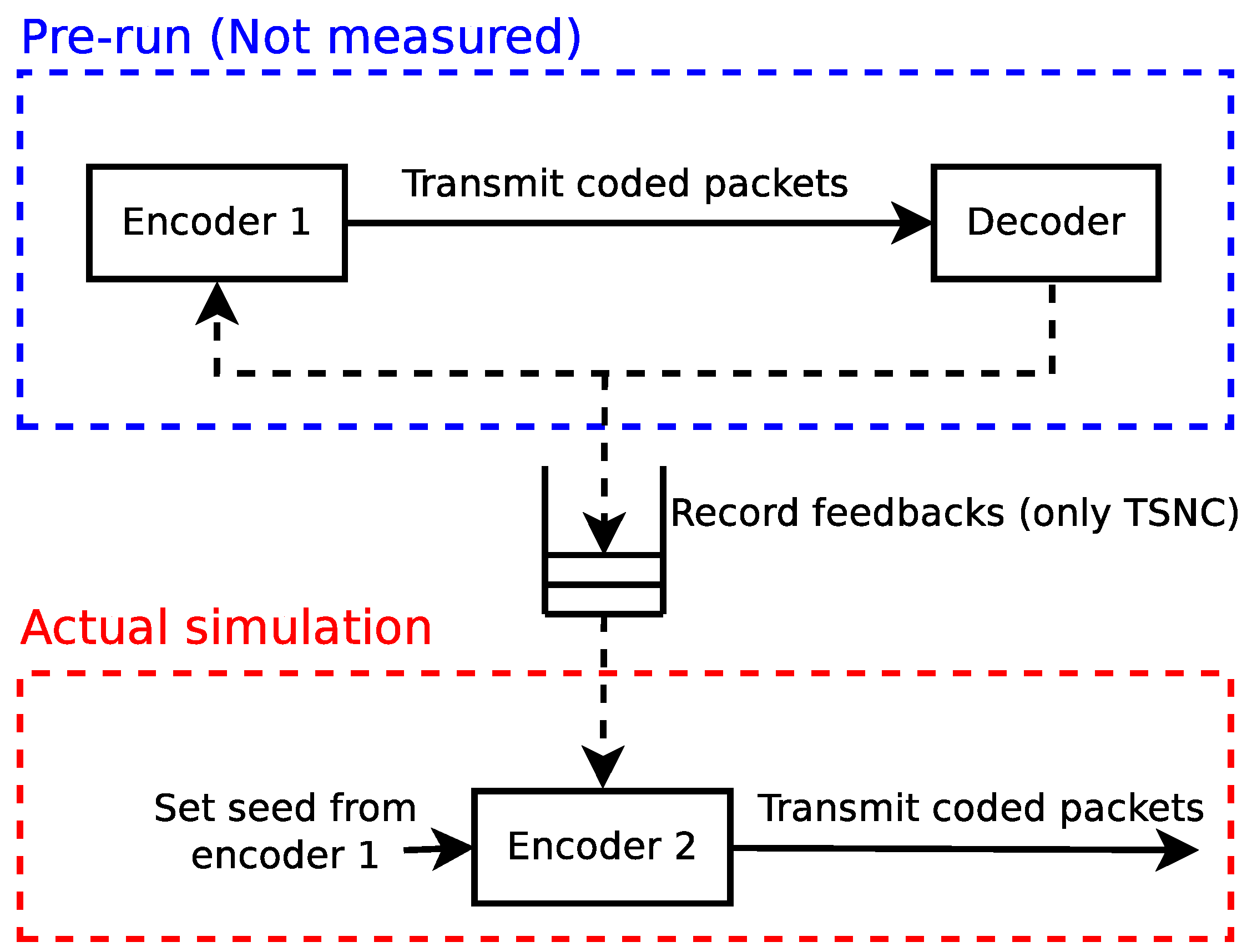
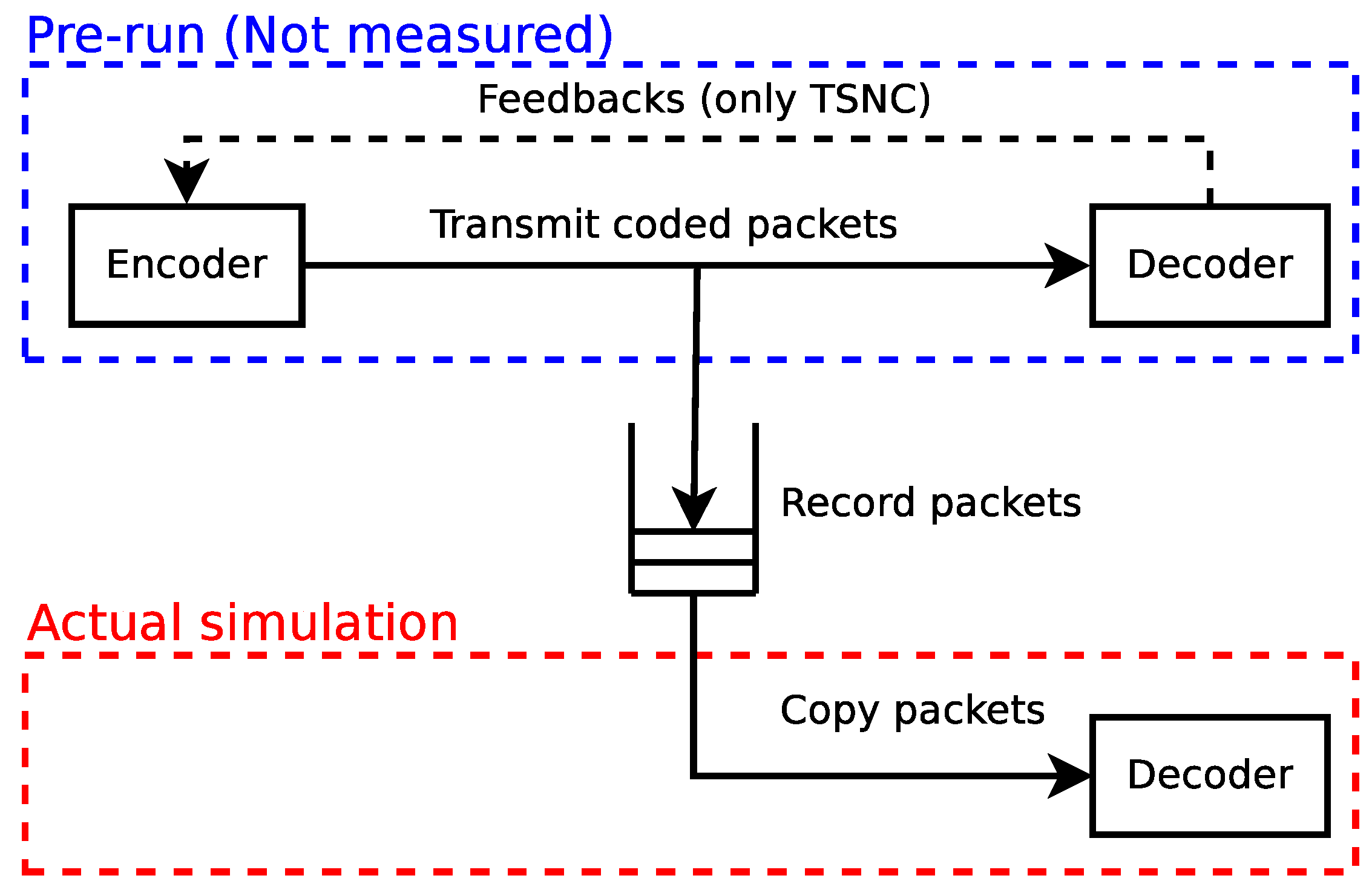
3. Metrics and Measurement Methodology

Once having defined the coding schemes behavior in terms of encoding and decoding, we proceed to describe the metrics considered in our study. The goodput is a measure for the effective processing speed, since it excludes protocol overhead, but considers all delays related with algorithmic procedures, field operations, hardware processing, multicore coordination (where it applies), etc. Moreover, both encoding and decoding goodput permit one to observe if coding is a system-block that limits the end-to-end performance. If a system presents a low goodput, this will affect the Quality of Experience (QoE) of delay-intolerant applications for the end user. For example, mobile user applications are typically delay-intolerant. Furthermore, Raspi processors are based on the ARM architecture, which is the same as in mobile devices, such as smartphones or tablets. Thus, the Raspi might be used as an experimental tool to get an estimate of the mobile device processing capability, which is easy-deployable and at a much lower cost than a smartphone.

To complement our study, we review the energy consumption of the Raspi, since this platform is deployed at a large scale in scenarios where (i) energy is constrained to the lifetime of the device battery and (ii) the devices could be established in locations that are unavailable for regular maintenance. Typical use cases of these types of scenarios are sensor applications where devices are positioned for measurement retrieval without any supervision for large periods of time.

3.1. Goodput

We consider the goodput defined as the ratio of the useful delivered information at the application layer and the total processing time. We focus on the goodput considering only the coding process, i.e., we assume that the application data have been properly generated before encoding and also correctly post-processed after decoding. In this way, we define the goodput for either an encoder or a decoder as follows:

$$\begin{array}{c}\hfill R_{proc}=\frac{gB}{T_{proc}}[\mathrm{Byte}/\mathrm{second}]\end{array}$$

(14)

In (14), B and g are the packet and generation size, as defined previously, and both represent the data to be processed. For goodput measurements, we are concerned with quantifying the processing time for either encoding or decoding g linearly-independent packets. Thus, $T_{proc}$ is the processing time required for this processing. In the next subsections, we define two time benchmarks available in [40]. The purpose of the benchmarks is to quantify the processing time for any of the coding schemes considered in Section 2.

3.1.1. Encoding Benchmark

Figure 1 refers to the benchmark setup made for measuring the encoding processing time. The time benchmark is divided into two parts as a way to exclude the decoding processing time from the measurements. In the first part, called a pre-run, we quantify the amount of transmitted coded packets, from Encoder 1 in Figure 1, required for decoding a generation of packets in a single encoder-decoder link with no packet erasures for a defined configuration of coding scheme, coding parameters and amount of feedback. In the case of TSNC, we also record the feedback packets received from the decoder. The purpose of the pre-run is to observe how an encoder behaves with a given seed within its random number generator. This part of the benchmark is not measured.

The second part is the actual simulation. The objective of this part is to replicate the pre-run to obtain the encoding speed without spending time decoding the packets. A Reset Encoder 2 in Figure 1 is given the same seed as in the pre-run, and then, we measure the time from which the process start until we reach the amount of transmitted packets in the pre-run. The measurement is stored as the encoder $T_{proc}$ for this generic configuration. For TSNC simulations, the recorded feedback packets are injected according to the observations in the pre-run.

3.1.2. Decoding Benchmark

Figure 2 shows the benchmark setup for measuring the decoding processing time. The time benchmark is divided into two parts as its encoding counterpart, e.g., a pre-run and the actual simulation. However, some differences occur.

In the pre-run, we still quantify the amount of transmitted coded packets from Encoder 1. Notice that we include the feedback case because it is necessary for the TSNC scheme. However, now, we store the transmitted packets instead. The reason being that we want to feed the decoder with the same packets in the same order. Later, in the actual simulation, a new decoder is given the same packets in the same order from the pre-run, and then, we measure the time from which the process starts until the decoder finishes to retrieve the original packets. Finally, this measurement is saved as the decoder $T_{proc}$ for this general configuration.

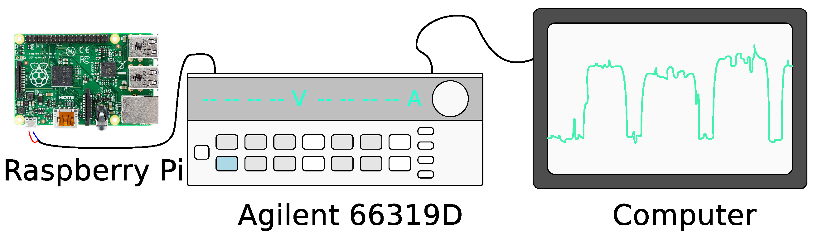
3.2. Energetic Expenditure

In large-scale networks where several Raspis might be deployed, both average power and energy per bit consumption of the devices are relevant parameters that impact the network performance for a given coding scheme. Hence, we consider a study of these energy expenditure parameters for the encoding and decoding. We define these metrics and propose a setup to measure them.

The average power specifies the rate at which energy is consumed in the Raspi. Thus, for a given energy value in the device battery without any external supplies, this metric permits one to infer the amount of time for which the Raspi can operate autonomously before draining out its battery. For the energy per bit consumption, it indicates how much energy is expended to effectively transmit or receive one bit of information taking into account the encoding or decoding operations, respectively.

For our energy measurement campaign, we automate the setup presented in Figure 3 to sequentially run a series of simulations for a given configuration of a coding scheme and its parameters, to estimate the energetic expenditure in both of our Raspi models. The energy measurement setup goal is to quantify the energy consumption of the Raspi over long periods of processing time to obtain accurate results. A representative sketch of the setup is shown on the computer monitor in Figure 3.

The energy measurement setup presents a Raspi device whose power supply is an Agilent 66319D Direct Current (DC) source, instead of a conventional power chord supply. To compute the power, we just need to measure the current, since the Raspi feeds from a fixed input voltage of 5 V set by the Agilent device, but its electric current demand is variable. Hence, the measured variable is the current consumed by the device for this fixed input voltage. The output of the measurements are later sent to a workstation where the raw measurement data are processed.

To identify each experiment, we classified the electrical current samples into two groups based on the magnitude. In our measurements, the groups to be reported are the idle current $I_{idle}$ and the processing current $I_{proc}$. The former is the current the Raspi requires while in idle state, meaning that no processing is being carried out. The latter stands for the current needed during the encoding or decoding processing of the packets. Measurements are taken either when $I_{idle}$ or $I_{proc}$ are observed. For the processing currents, its current measurements are made while the goodput benchmarks are running for a given configuration of a coding scheme with its parameters. For each configuration, ${10}^3$ simulations from the goodput benchmarks are carried out during the period of time where $I_{proc}$ occurs. We remark that a simulation is the conveying of g linearly-independent coded packets. Finally, for each configuration, each set of current measurements is enumerated to map it with its average power value and the corresponding goodput measurements. At post-processing, from the average power expenditure and the results from the goodput measurements, it is possible to extract the energy per bit consumption. We elaborate further on this post-processing in the next subsections.

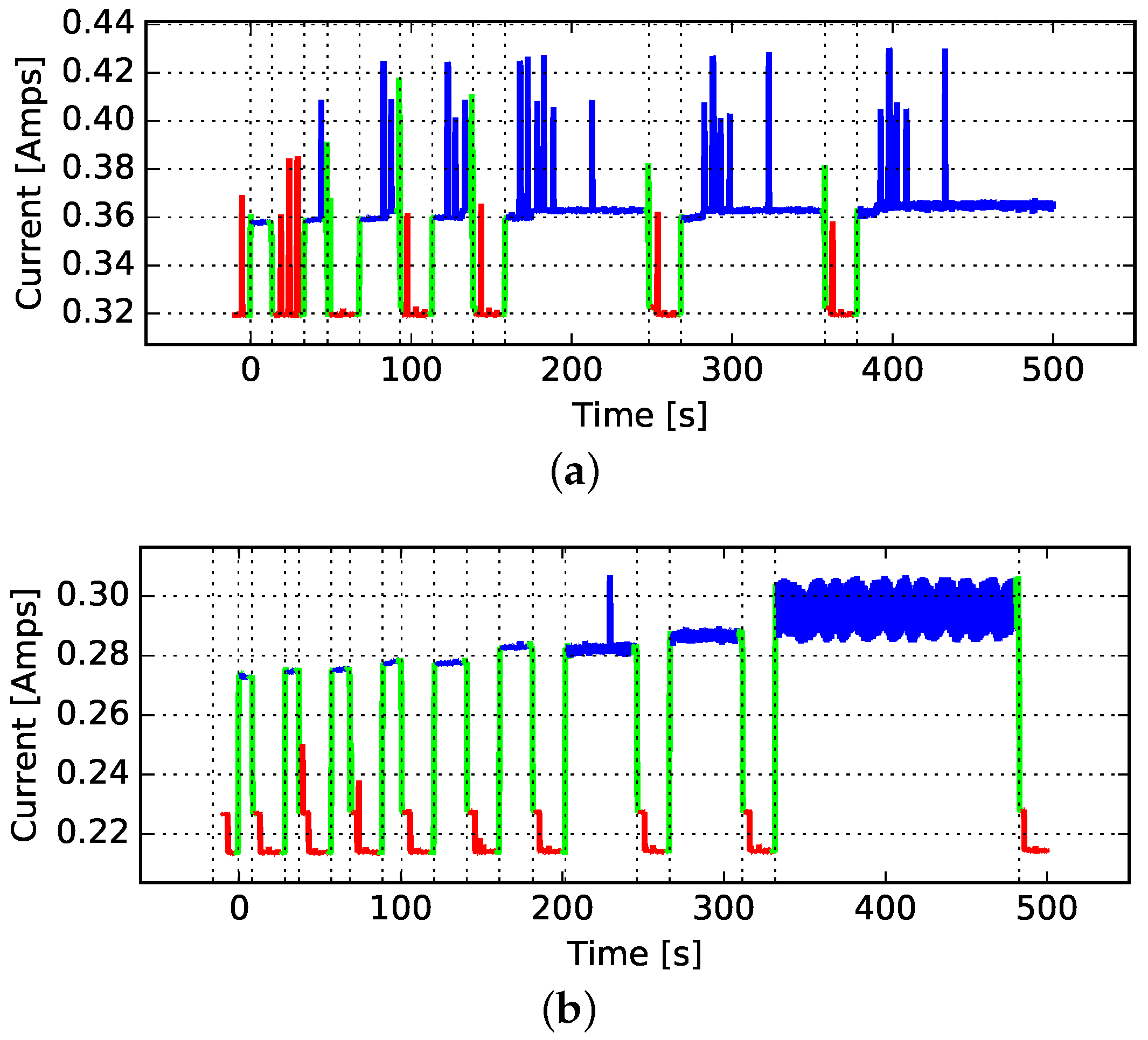
3.2.1. Average Power Expenditure

To extract the average power for a given configuration in our setup, we first calculate the average current in the idle state $I_{idle,avg}$ and the processing state $I_{proc,avg}$ for all of the available sample for the given configuration. Regardless of the current type, the average value of the sample set of a given number of samples $N_s$ is:

$$\begin{array}{c}\hfill I_{avg}=\frac{1}{N_s}\sum _{k=1}^{N_s}{I}_k\left[\mathrm{Ampere}\right]\end{array}$$

(15)

With the average current from (15), we compute the average current used for processing with respect to the idle state, by subtracting $I_{idle,avg}$ from $I_{proc,avg}$. Then, the result is multiplied by the supply voltage to obtain the average power during the considered configuration, given as:

$$\begin{array}{c}\hfill P_{avg}=V_{supply}(I_{proc,avg}-I_{idle,avg})\left[\mathrm{Watt}\right]\end{array}$$

(16)

3.2.2. Energy per Bit Consumption

To get this metric for a given configuration, we express the energy as the product of the average power by the processing time $T_{proc}(\mathrm{s}/\mathrm{byte})$ obtained from the goodput measurement for the same configuration. In this way, we can relate the processing time with the goodput, the packet and the generation size as shown:

$$\begin{array}{c}\hfill E_b=P_{avg}{T}_{proc,bit}=P_{avg}\times \frac{T_{proc}}{8gB}=\frac{P_{avg}}{8R_{proc}}\left[\mathrm{Joule}\right]\end{array}$$

(17)

4. Measurements and Discussion

With the methodology and setups from the previous sections, we proceed to obtain the measurements for the Raspi 1 and 2 devices. We consider the following set of parameters for our study: For all of the codes, we use $g=[16,32,64,128,256,512]$ and $q=[2,2^8]$. For the single-core implementations and cases when the generation size is varied, $B=1600$ bytes. We consider another setup where only the packet size varies, $B=[64,128,$$256,512,1024,2048,4096,8192,16,384,32,768,65,536,131,072]$ bytes with a generation size fixed on $g=[16,128]$ to see the performance of the Raspis in low and high packet size regimes. The third setup we considered used $B=1536$ bytes for the optimized multicore implementation. SRLNC was measured with the densities $d=[0.02,0.1]$. For TSNC, we considered excess packets, $e=[8,16]$, so that the budget is $b=g+e$. In all our measurement reports, to simplify their review, we first present the results for the Raspi 1 and later continue with the Raspi 2.

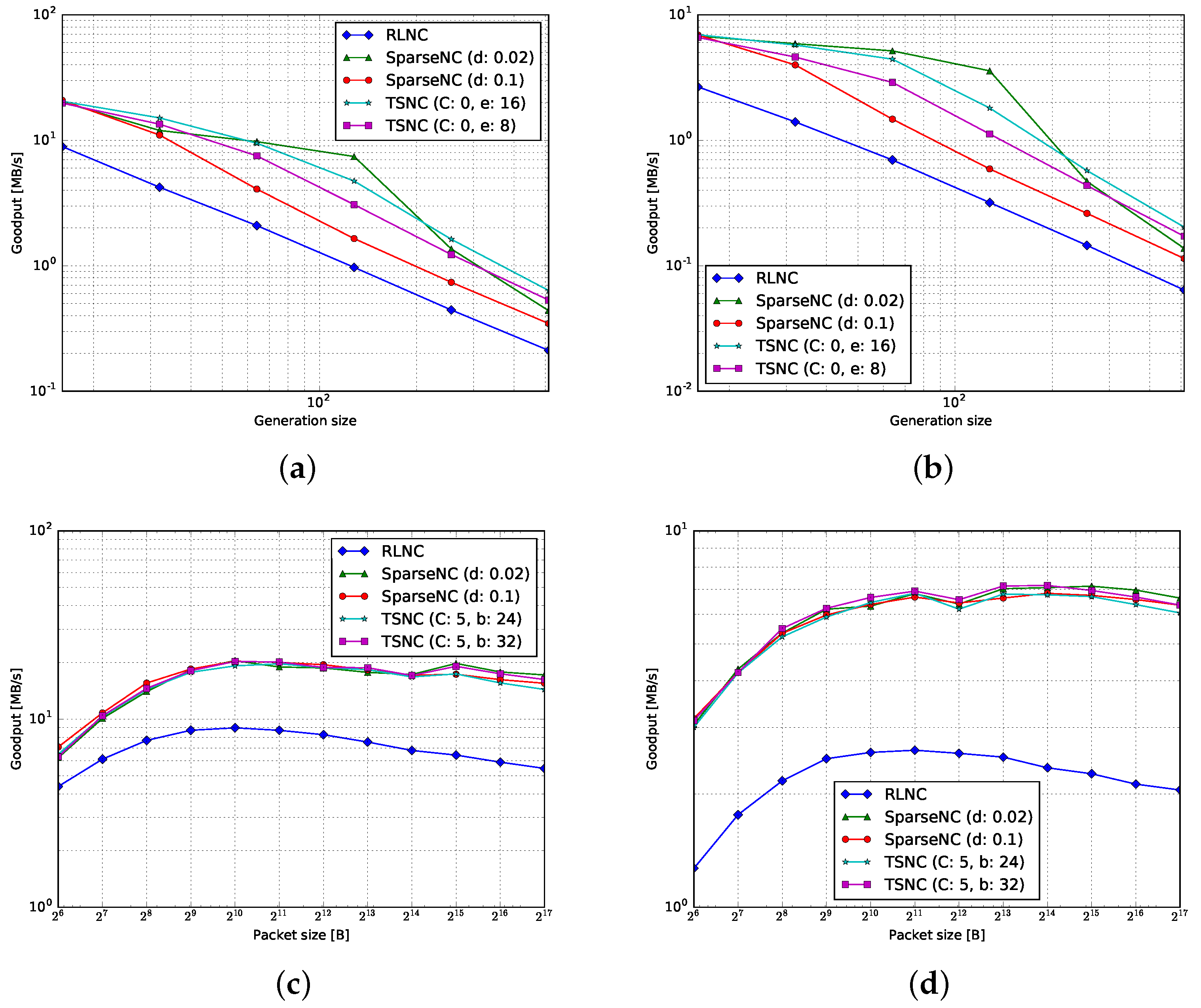
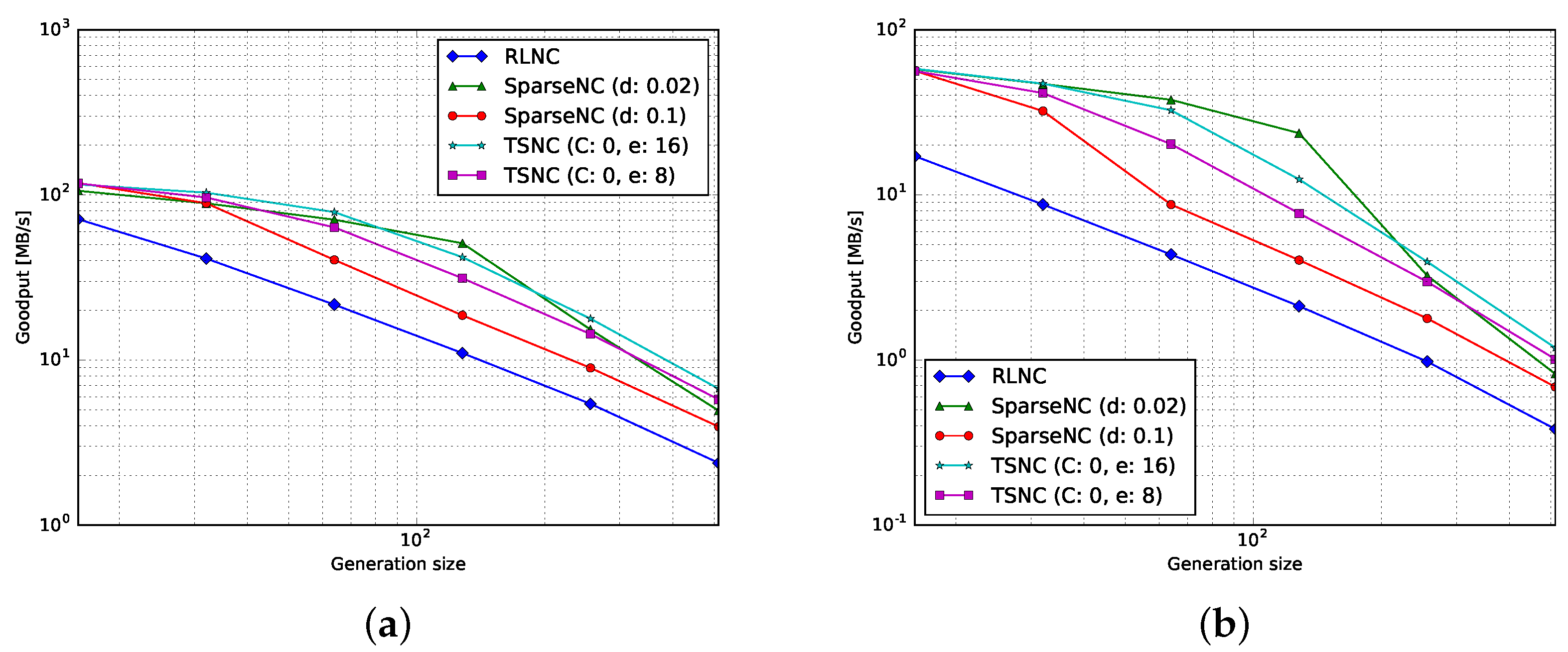
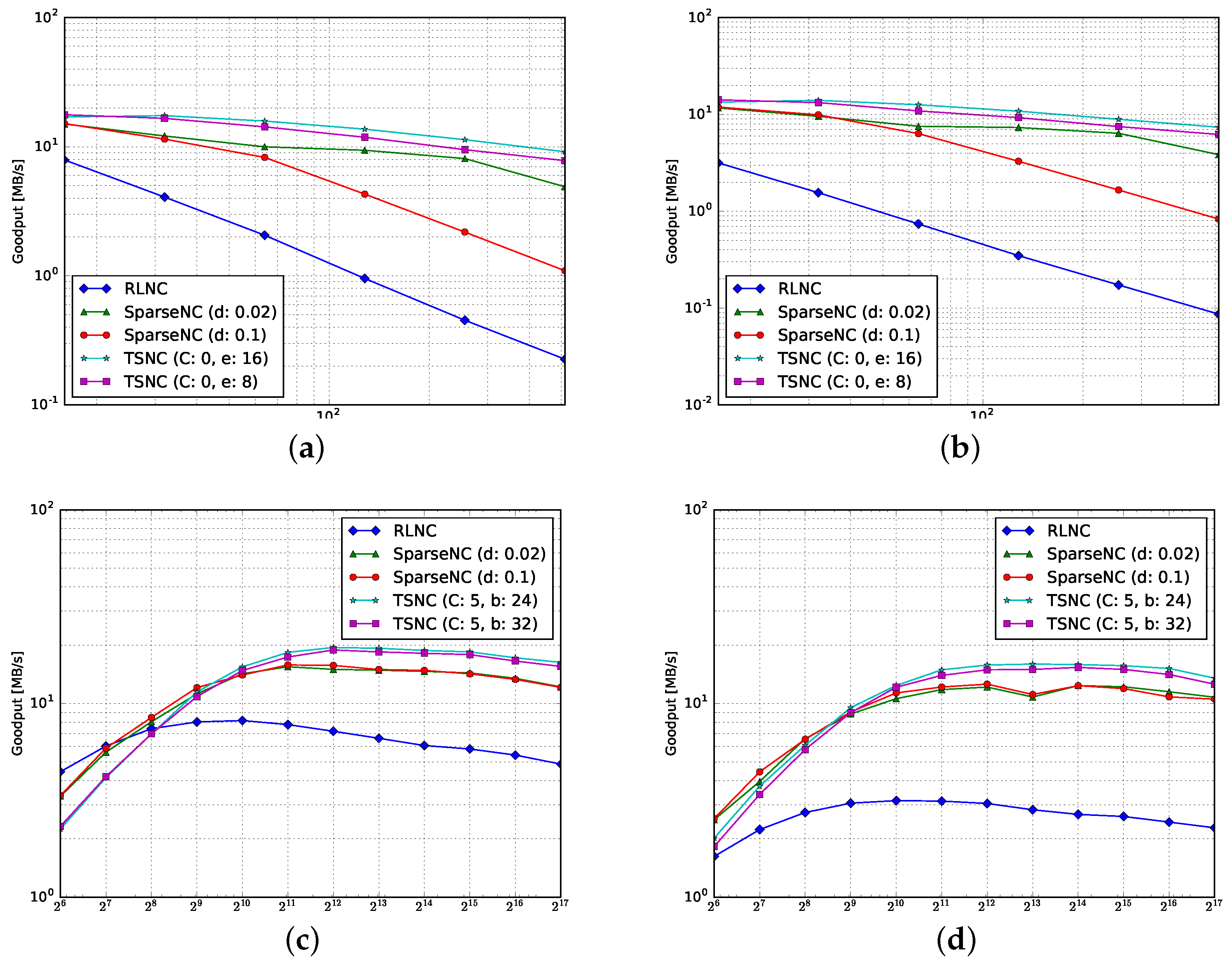
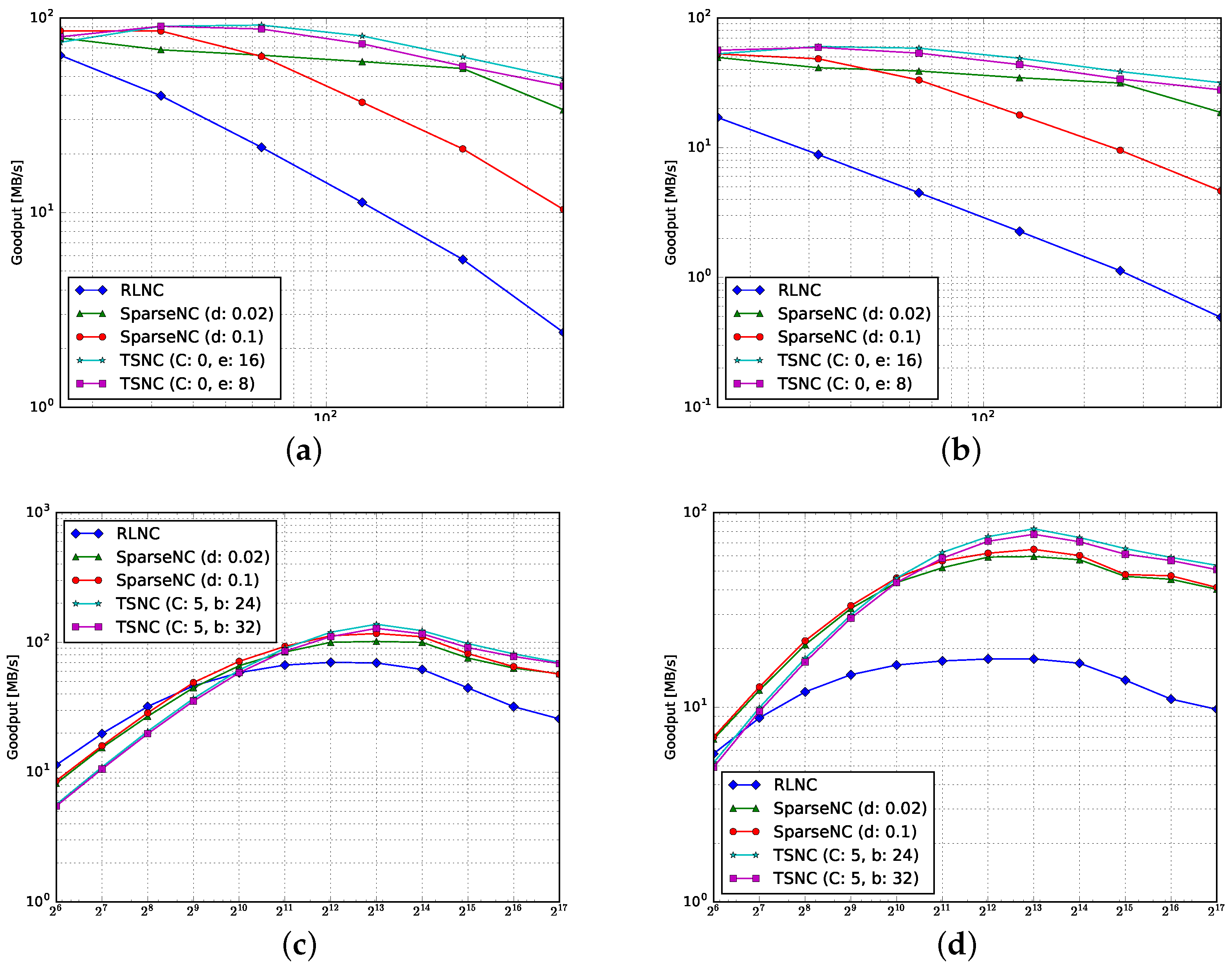
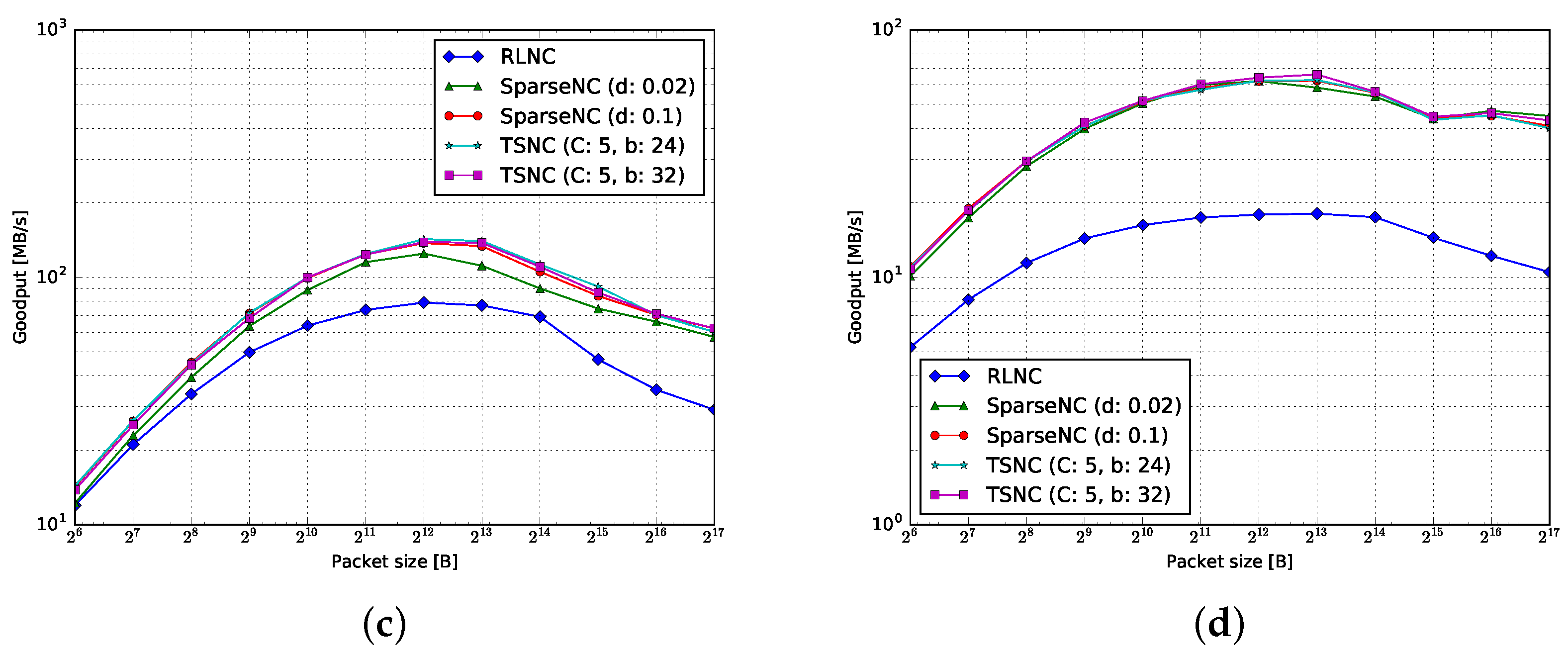
4.1. Goodput

For the goodput, we separate the results according to their time benchmarks as we did in Section 3. We proceed first with the measurements related to the encoder and later review the case of the decoder.

4.1.1. Encoding

Figure 4 shows the results of the encoder goodput measurements for the Raspi 1. Figure 4a,b presents goodput as a function of the generation size for $GF\left(2\right)$ and $GF\left(2^8\right)$, respectively, for a packet size of $B=1600$ bytes. Figure 4c,d presents the same metric, but now as a function of the packet size for $GF\left(2\right)$ and $GF\left(2^8\right)$, respectively. In this case, the generation size was set to $g=16$ packets.

Similarly, Figure 5 shows the same set of measurements for the Raspi 2. Hence, Figure 5a,b presents goodput as a function of the generation size and Figure 5c,d as a function of the packet size for the same cases mentioned previously. Therefore, we will proceed to make the results analysis with Raspi 1 and indicate which similarities or differences occur for the Raspi 2 and when they occur.

As can seen from Figure 4a,b and Figure 5a,b, which indicate the goodput dependency on the generation size, the encoding goodput gets reduced as the generation size increases, regardless of the Raspi model observed. The reason is that the encoding operation processing is $\mathcal{O}\left(g\right)$ because it is required to create g coding coefficients and to do g multiplications for each packet. This makes the goodput scale as the inverse of the generation size.

In the sets of figures shown in Figure 4 and Figure 5, it can be observed that the goodput for $GF\left(2\right)$ is higher than for $GF\left(2^8\right)$, but still around the same order of magnitude. This difference is explained by noticing that GF arithmetics in the binary field are simply XOR or AND operations. These operations are implemented efficiently in architectures nowadays. However, the operations in $GF\left(2^8\right)$ are more complex given that the finite field arithmetics have to be performed with lookup tables, which at the end reduces the computing speed giving a lower goodput when compared with the binary field.

In Figure 4a,b and Figure 5a,b, it can be seen that the goodput trends of five codes are a function of the generation size: RLNC, SRLNC with $d=[0.02,0.1]$ and TSNC, with an extra parameter that we mention. We define C as the number of density regions in the TSNC transmission process. The maximum number of possible regions depends on the generation size (12). The larger the generation, the more density regions may be formed and the more density changes are possible. Throughout this paper, TSNC is configured to use the maximum number of density regions possible. As there can be at least $C=1$ density region in a transmission, we use $C=0$ to indicate the maximum possible density regions. This is used for TSNC in plots where the generation size is not fixed. For the plots in the mentioned figures from the encoder goodput measurements, RLNC presents the lowest performance in terms of goodput and TSNC with $e=16$, the highest regardless of the Raspi model. Given that the processing time depends on the amount of coded packets required to be created, RLNC is the slowest to process since it must use all of the g original packets. Later, sparse codes process the data at a larger rate since less packets are being mixed when creating a coded packet. The caveat of these schemes is that the sparser the code, the more probable the occurrences of linearly-dependent packets are. Therefore, basically, the sparser the codes, the more overhead due to the transmissions of linearly-dependent packets. Excluding the coding coefficients overhead, the overhead due to transmissions of linearly-dependent packets might be high for the sparse schemes. For example, if we consider TSNC with $e=16$ and $g=16$ in Figure 4a, the budget in this case permits one to send up to 32 packets, which is $2\times$ the generation size for an overhead of $100\%$ excluding the overhead from appending the coding coefficients. This happens because TSNC has been allowed to add too much redundancy in this case. For RLNC, this is not the case, since the occurrence of linearly-dependent coded packets is small, because all coding coefficients are used. Even for $GF\left(2\right)$, the average amount of redundant packets for RLNC has been proven to be 1.6 packets after g have been transmitted [41,42], but less than the cases where sparse codes are utilized. Overall, we observe that there is a trade-off between goodput and linearly-dependent coded packets’ transmission overhead.

For Figure 4c,d and Figure 5c,d, we see the packet size effect in the encoding goodput in both Raspi models and for a fixed generation size. For TSNC in this case, we allow for five density changes during the generation transmission and again consider the same budgets as before. In all of the cases, we observe that there is an optimal packet size with which to operate. When reviewing the specifications of the Raspi 1, it uses an L1 cache of 16 KiB. Hence, the trends in the packet size can be explained in the following way: For low packet sizes, the data processing does not overload the Central Processing Unit (CPU) of the Raspi, so the goodput progressively increases given that we process more data as the packet size increases. However, after a certain packet size, the goodput gets affected, since the cache starts to saturate. The packets towards the cache needs to have more processing. Beyond this critical packet size, the CPU just queues processing, which incurs larger delay reducing the goodput.

If we consider the previous effect when reviewing the trends in the mentioned figures, in all of the models, we observe that the maximum coding performance is not at 16 KiB, but at a smaller value depending on the model, field size and coding scheme considered. The reason is that the CPU needs to allocate computational resources to other processes from the different tasks running in the Raspi. Then, given that there are various tasks from other applications for proper functioning running in the Raspi at the same time as coding, the cache space is filled also with the data from these tasks, thus diminishing the cache space available for coding operations.

For the Raspi 1 model, we observe in Figure 4c that the critical packet size for RLNC using $GF\left(2\right)$ occurs at 1 KiB, whereas for the sparse codes, it is close to 8 KiB in most cases for $GF\left(2\right)$. This difference takes place since the sparse codes mix less packets than RLNC, which turns into less data loading in the cache for doing computations. For a density of $d=0.1$, a packet size of $B=8$ KiB and $g=16$ packets, we observe that roughly $⌈gd⌉=2$ packets are inserted in the cache when calculating a coded packet with this sparse code. Loading this into the cache, this stands for 16 KiB, which is the cache size. A similar effect occurs for the other sparse codes. However, for RLNC given that it is a dense code since $d\to 1$, RLNC packets load data from all of the $g=16$ coding coefficients, which accounts for the 16 KiB of the cache size. In Figure 4d, although the ideal packet size remains the same for RLNC and the sparse codes, the final goodput is lower due to the field size effect.

The effects mentioned for the Raspi 1 were also observed for the Raspi 2 as mentioned previously. Still, the Raspi 2 achieves roughly $5\times$ to $7\times$ gains in terms of encoding speed when comparing the goodputs in Figure 4 and Figure 5, given that it has an ARM Cortex A7 (v7) CPU and twice the Random Access Memory (RAM) size than the ARM1176JZF-S (v6) core of the Raspi 1 model.

In Figure 5c,d, we observe that the packet size for the maximum RLNC goodput has shifted towards 8 KiB, indicating that the Raspi 2 is able to handle $16\times 8$ KiB $=128$ KiB. This is possible because the Raspi 2 has a shared L2 cache of 256 KiB allowing it to still allocate some space for the data to be processed while achieving a maximum goodput of 105 MB/s.

4.1.2. Decoding

Similar to the encoding goodput, in this section, we review decoder goodput in terms of performance and configurations. Figure 6 shows the results of the decoder goodput measurements for the Raspi 1 and Figure 7 for the Raspi 2.

In Figure 6 and Figure 7, we observe the same generation and packet size effects reported in the encoding case. However, we do observe in Figure 6a,b and Figure 7a,b that doubling the generation size does not reduce the goodput by a factor of four. In principle, given that Gaussian elimination scales as $\mathcal{O}\left(g^3\right)$ (and thus, the processing time), we would expect the goodput to scale as $\mathcal{O}\left(R_{proc,dec}\right)=\mathcal{O}(g/g^3)=\mathcal{O}\left(g^{-2}\right)$. This would imply that doubling the generation size should reduce the goodput by a factor of four, which is not the case. Instead, the goodput is only reduced by a factor of two. This is only possible if the Gaussian elimination is $\mathcal{O}\left(g^2\right)$. A study in [23] for RLNC speeds in commercial devices indicated that this is effectively the case. The reason is that the $g^2$ scaling factor in the scaling law of the Gaussian elimination is much higher than the $g^3$ scaling for $g<512$. Particularly, this factor relates to the number of field elements in a packet size as mentioned in [23].

Another difference with the encoding goodput resulting in the same figures is that even though TSNC with $e=16$ packets provides the fastest encoding, it does not happen to be the same for the decoding. For this very sparse scheme, the decoding is affected by the amount of linearly-dependent packets generated, which leads to a higher delay in some cases (particularly in $g=[64,128]$). For other generation sizes, the performance of sparse codes is similar.

4.2. Average Power

With the energy measurement setup described in Section 3.2, we compute the average power of each device from their electric current consumption across time in Figure 8a,b. In each figure, the electric current values are classified into three possible currents: idle, transition and processing. These values are identified by our post-processing. Later, the values in red are idle currents, green for transitions and blue for processing.

For a given configuration of a coding scheme, device type and its parameters, only electrical current processing values are present. In general, we associate the current samples from a given configuration with its goodput through a timestamp. In this way, we relate goodput and power/energy measurements. Once having identified the electric current values, we compute the averages for each configuration as described in Section 3.2. In the presented current samples, we observe the presence of bursty noise. Nevertheless, by taking the average as described in (15), we remove this contribution in the average processing current.

By reviewing the processing current samples in Figure 8a,b, we observe that the average processing current does not change significantly for each Raspi model in all of the shown configurations. Therefore, we approximate the electric current consumption for the devices and compute the average power as indicated in (16). The results are shown in

Table 1. Average power for the Raspi models.

Raspi Model	${\mathit{I}}_{\mathit{i}\mathit{d}\mathit{l}\mathit{e},\mathit{a}\mathit{v}\mathit{g}}$ (A)	${\mathit{I}}_{\mathit{p}\mathit{r}\mathit{o}\mathit{c},\mathit{a}\mathit{v}\mathit{g}}$ (A)	${\mathit{P}}_{\mathit{a}\mathit{v}\mathit{g}}$ (W)
Raspi 1	0.320	0.360	0.200
Raspi 2	0.216	0.285	0.345

.

From Table 1, we notice that the power expenditure for both models is almost the same. Thus, the energy behavior is mostly dependent on the goodput trends, since the power is just a scaling constant.

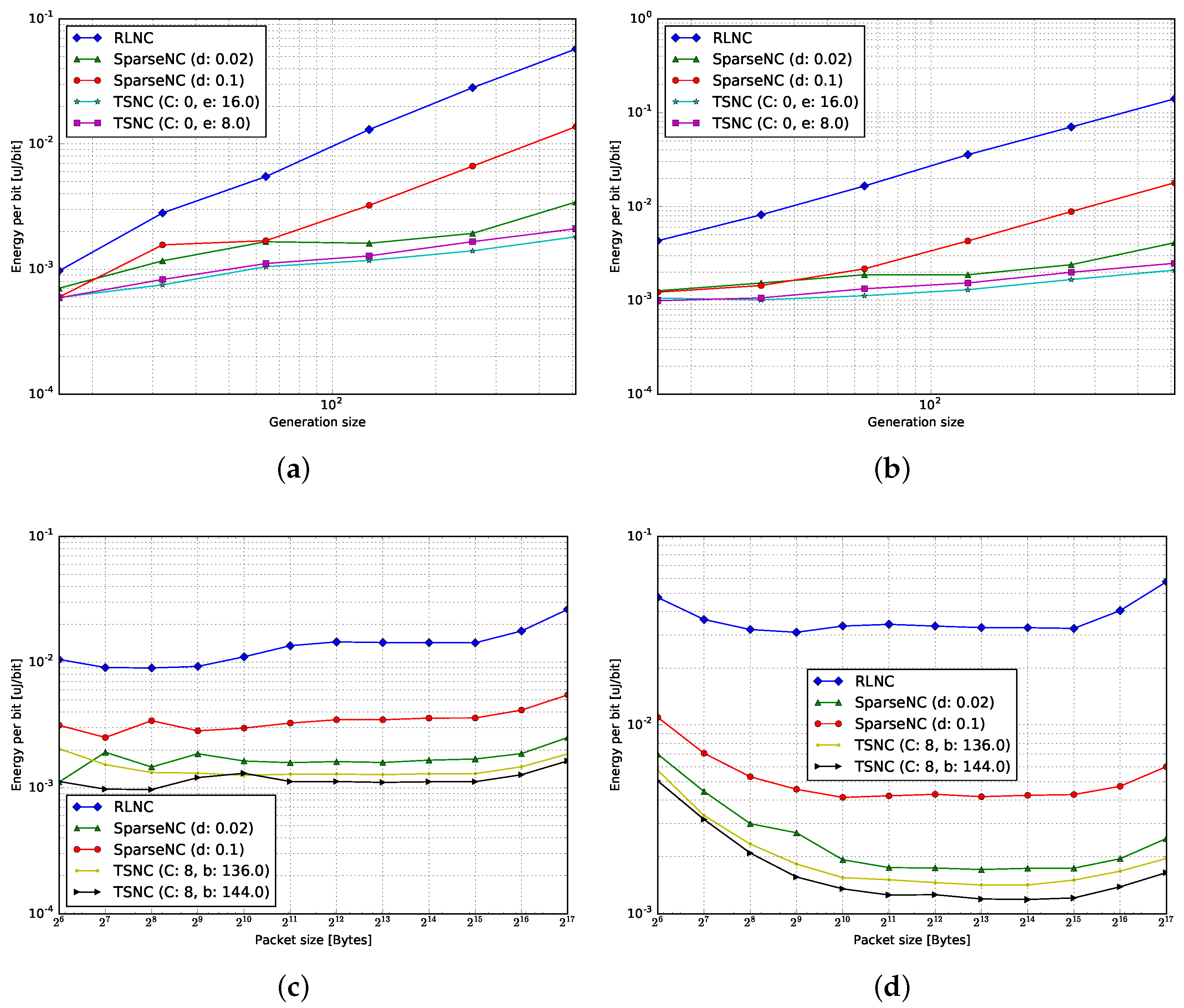
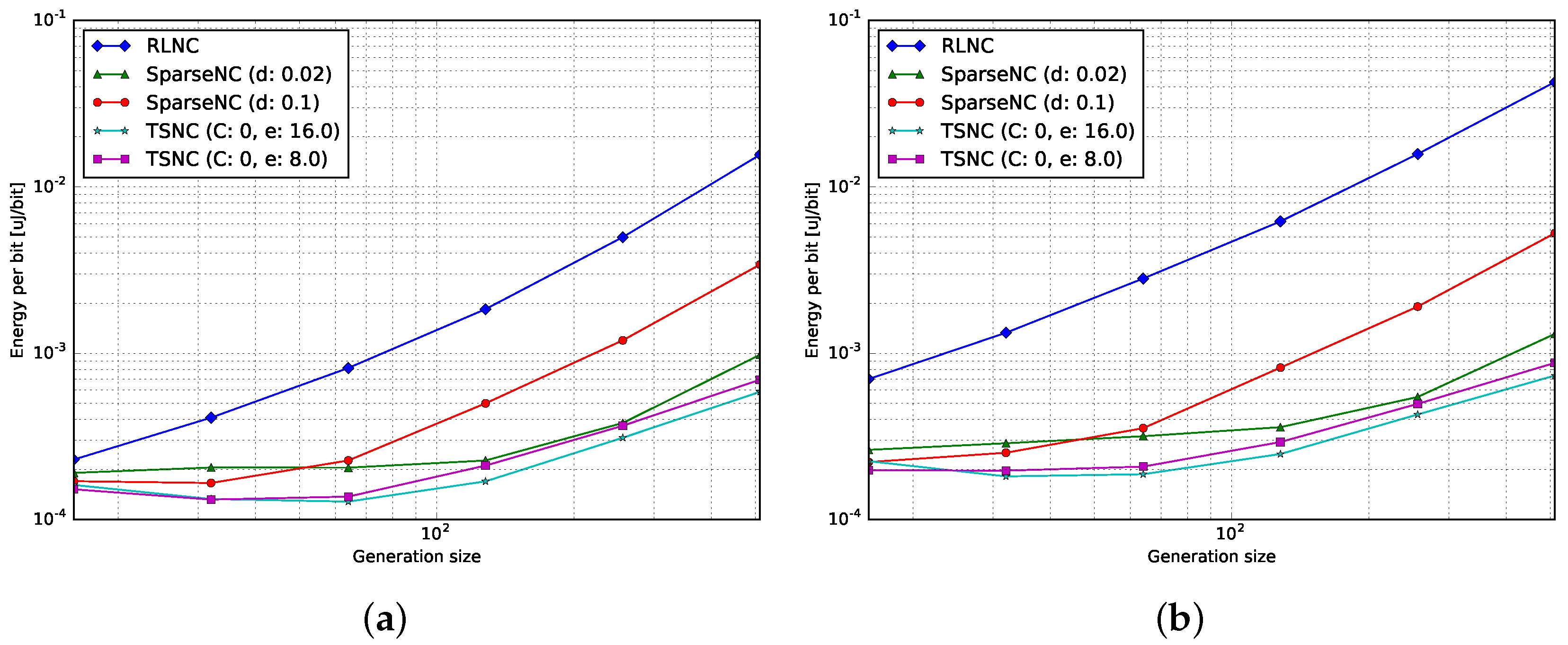
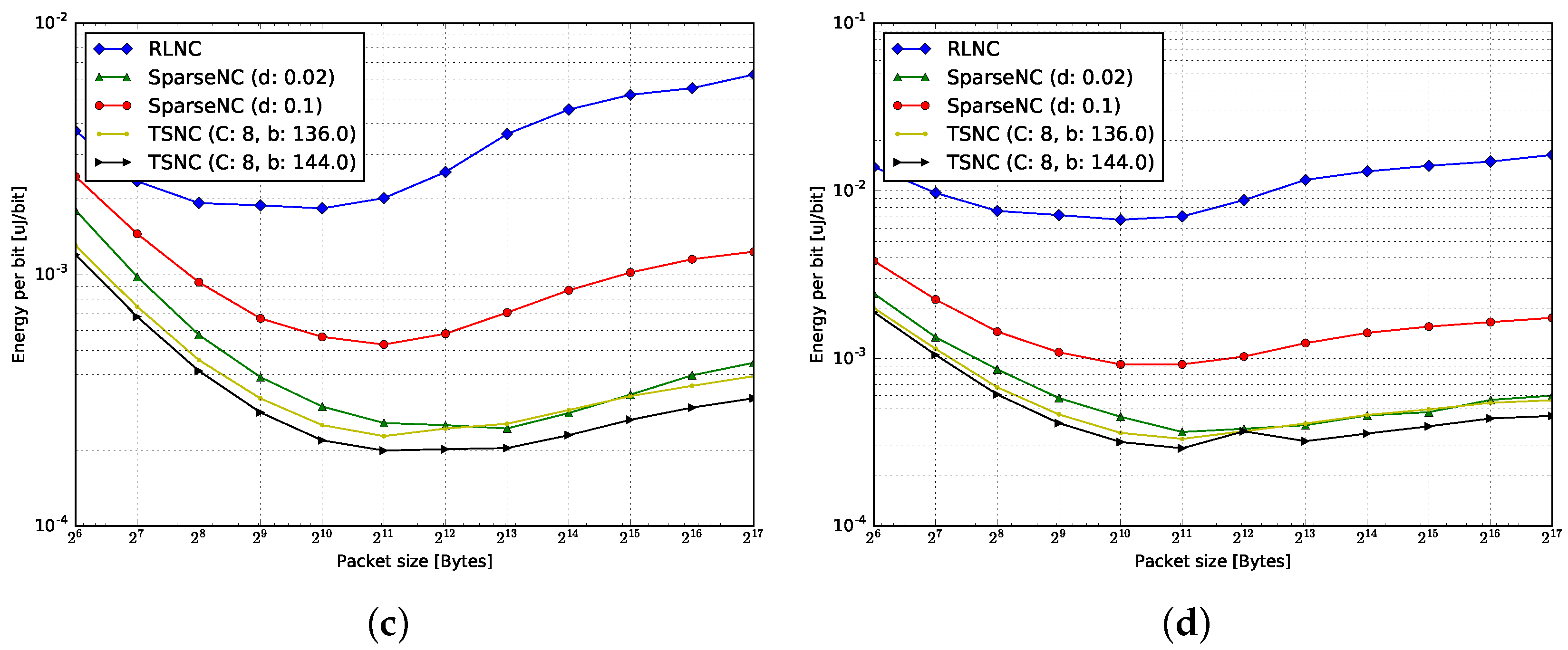
4.3. Energy per Bit

With power and goodput measurements, we compute the energy per bit of the previously-mentioned cases as described in (17). The trends of the energy per bit are the inverse of the goodput since both metrics are related by an inverse law. As made with the goodput, we separate the result descriptions according to the operation carried out by the Raspi: encoding and decoding. Besides this, we differentiate between the models in our study. The energy per bit consumption removes the dependency on the amount of packets, helping to normalize the results and indicating energy consumption on a fair basis for all of the configurations and coding operations involved in the study.

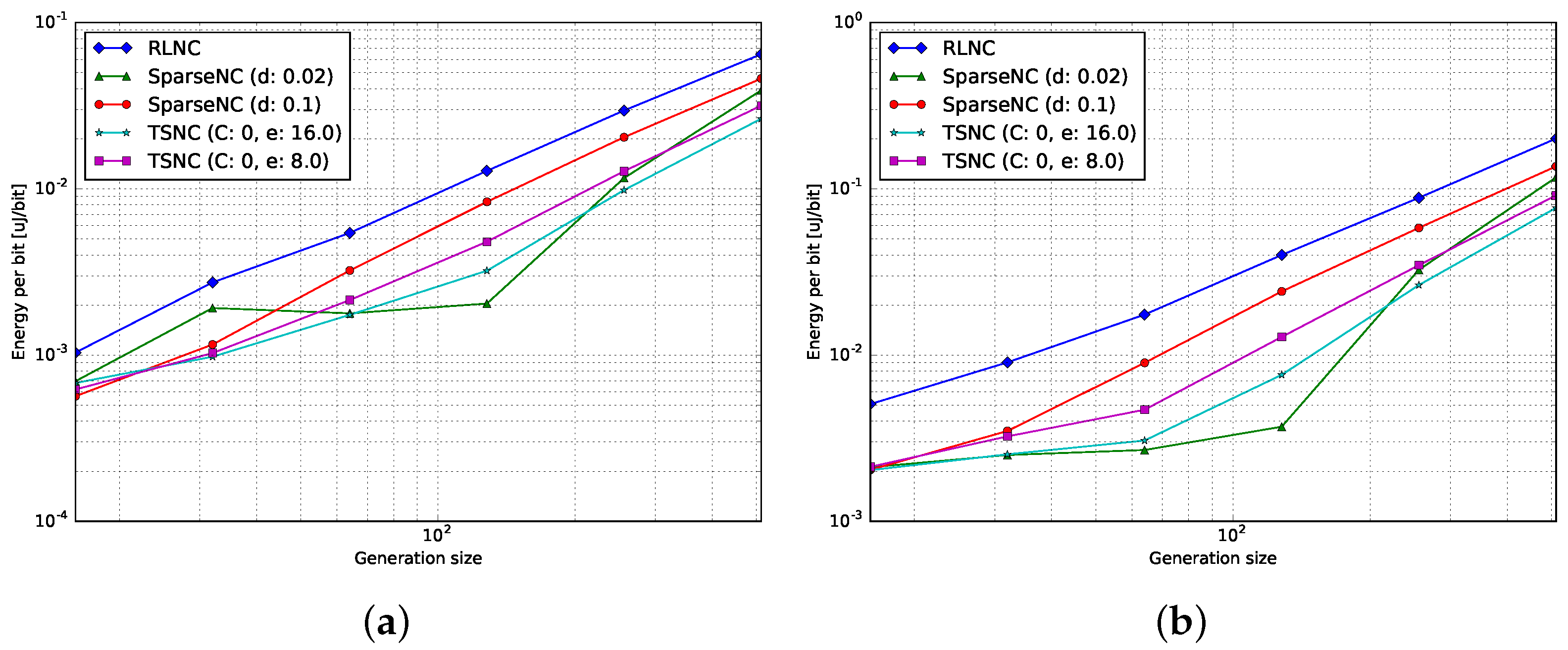
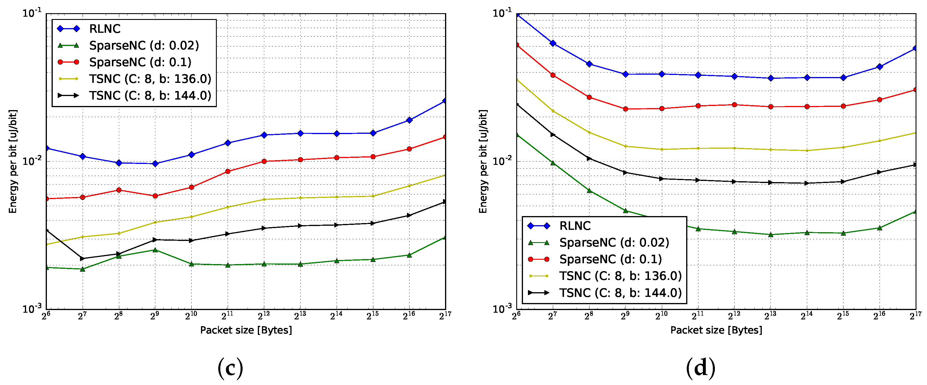
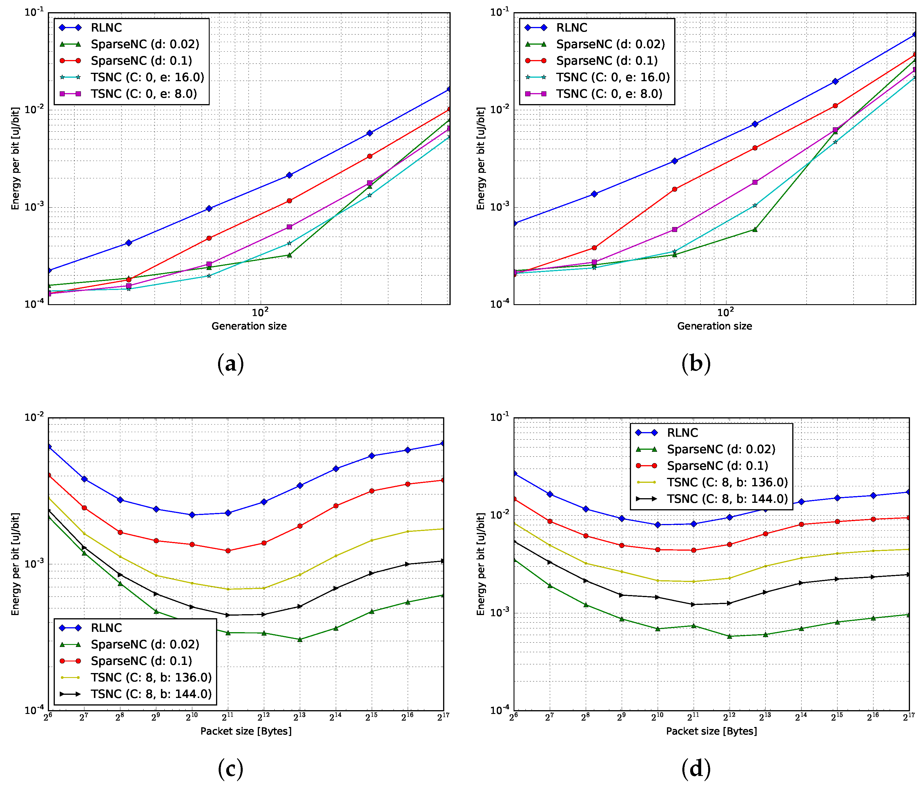
4.3.1. Encoding

Figure 9 and Figure 10 show the encoding energy per bit measurements for the Raspi 1 and 2 models, respectively. We now proceed to analyze first the Raspi 1 case pointing out proper differences with the Raspi 2 when applicable.

In Figure 9a,b, we see the dependency of the energy per bit processed on the generation size for the Raspi 1 model. In these types of plots, incrementing the generation size incurs more processing time per byte sent, which leads to more processing time per bit sent. For RLNC, the energy trends scale as the processing time scales, which is $\mathcal{O}\left(g\right)$. For sparse codes, this trend is scaled by the density, thus for sparse, we have $\mathcal{O}\left(⌈gd⌉\right)$, which can be appreciated in the same figures. We do also notice that using $GF\left(2\right)$ is energy-wise efficient on a per-bit basis since less operations are used to perform the GF arithmetics, which reduces the amount of energy spent.

In Figure 9c,d for the same device, we exhibit the relationship between the energy per bit processed on the packet size, which is the inverse of the goodput vs. the packet size scaling law. We set $g=128$ in this case to observe energy per bit consumption in the regime where the processing time is considerable. As we notice again in this case, $GF\left(2\right)$ presents as the field with the smallest energy per bit consumption given that is the one that has the least complex operations. The trends for the energy can be explained as follows: As the packet size increases, we process more coded bits at the same time, which increases the encoding speed, until we hit the critical packet size. After this value, we spend more time queueing data towards the cache besides the processing, which increases the time spent per processed bit and, thus, the energy.

In Figure 10a–d, we show the encoding energy per bit consumption for the Raspi 2. We clearly see that the effects discussed for the Raspi 1 also apply as well for the Raspi 2. Moreover, given that the average power is in the same order, but the Raspi 2 is a faster device, the energy costs for the Raspi 2 are $2\times$ less than the Raspi 1 when referring to variable generation sizes and a fixed packet size. Furthermore, these costs are one order of magnitude less for the Raspi 2 with respect to the Raspi 1 regarding the case of a fixed generation size and a variable packet size. This makes the Raspi 2 achieve a minimum encoding energy consumption per bit processed of 0.2 nJ for the binary field in the mentioned regime.

4.3.2. Decoding

In Figure 11a–d, we show the encoding energy per bit consumption for the Raspi 1. Again, we notice very similar behavior and trends as previously reviewed for the encoding energy per bit expenditure. In this case, we focus on performance among the coding schemes since the behavior and trends were previously explained for the encoding case. Later, we introduce the decoding energy results for the Raspi 2 doing relevant comparisons with the Raspi 1.

Some differences occur due to the nature of decoding. In this situation, the reception of linearly-dependent coded packets just increases the decoding delay, therefore reducing the performance of some coding schemes in terms of the energy per bit consumption. For example, we notice that using SRLNC with $d=0.02$ outperforms TSNC with $C=0$ and $e=16$, for most of the cases of the variable generation size curves and in all of the cases of the variable packet size curves of Figure 11. This is a clear scenario, where the decoding delay is energy-wise susceptible to the transmissions of linearly-dependent coded packets. With the Raspi 1, decoding energies per processed bit of 2 nJ or similar are possible.

Finally, in Figure 12a–d; we introduce the decoding energy per bit consumption for the Raspi 2. Here, we obtain a reduction of an order of magnitude in energy per processed bit due to the speed of the Raspi 2. For example, it can be seen that for the binary field with $g=16$ packets, we achieve a decoding energy consumption per bit processed close to 0.1 nJ in practical systems.

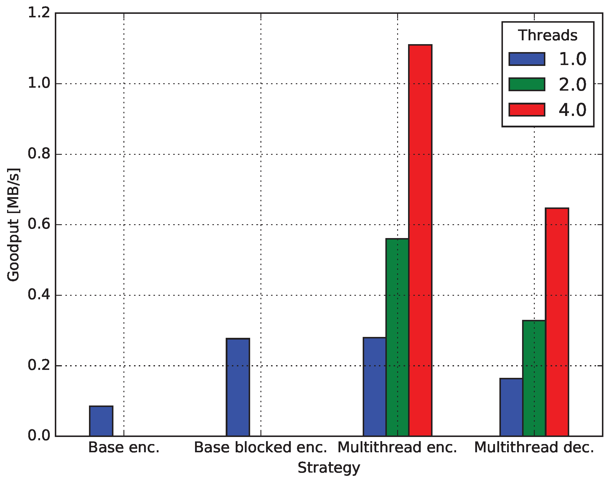
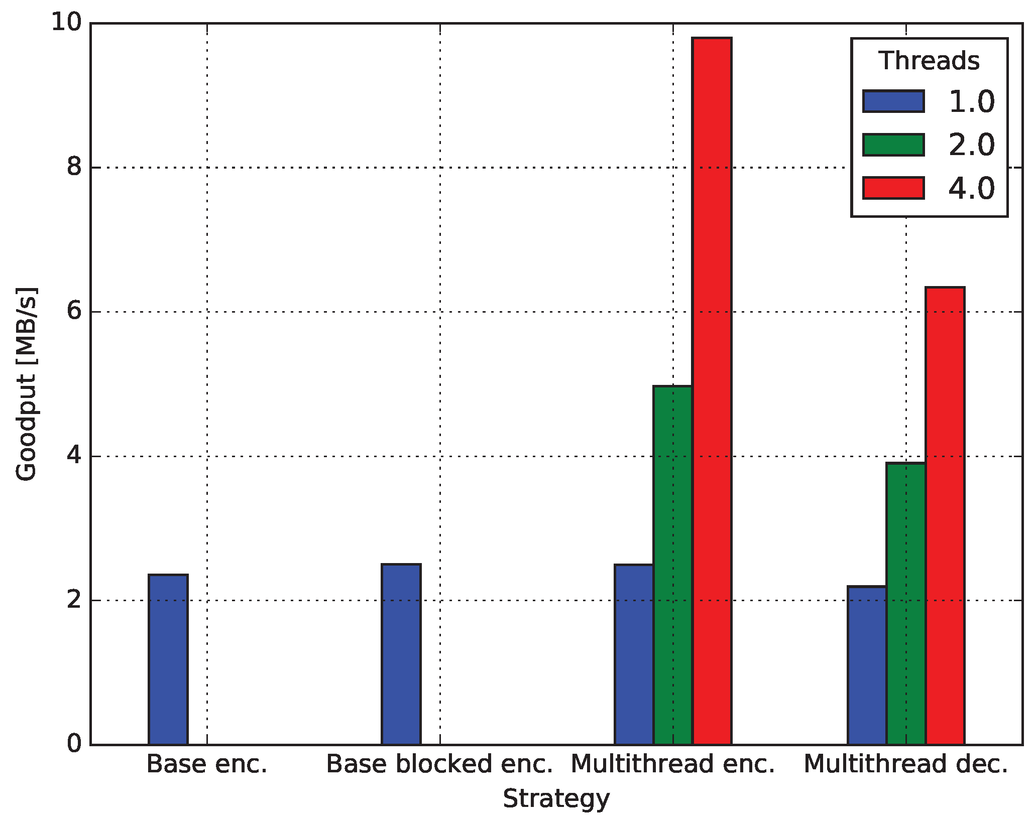
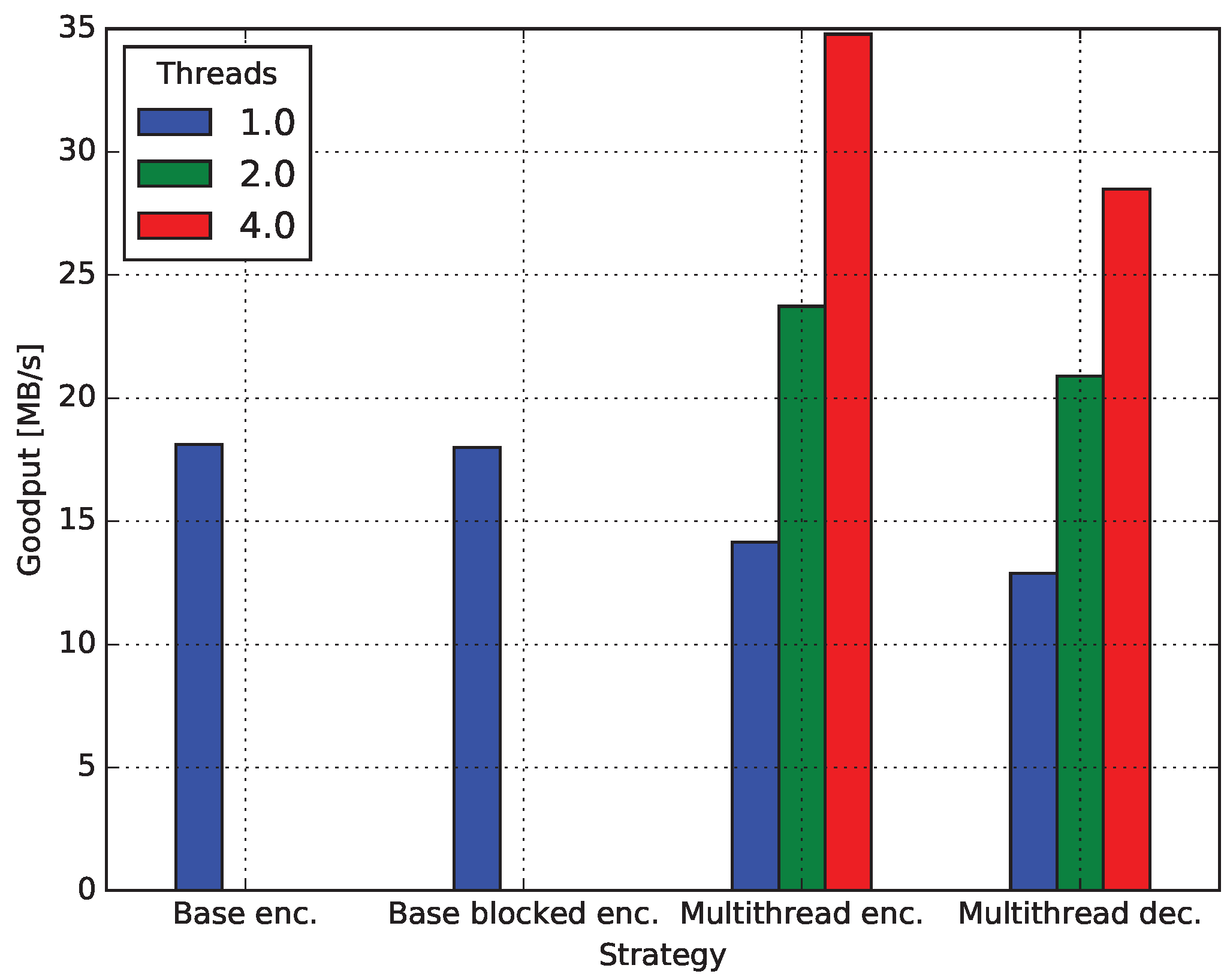
4.4. Multicore Network Coding

To review the performance of NC in a multicore architecture, we implemented the algorithm described in Section 2.4 on the Raspi 2 Model B, which features four ARMv7 cores in a Broadcom BCM2836 System on Chip (SOC) with a 900-MHz clock. Each core has a 32-KiB L1 data cache and a 32-KiB L1 instruction cache. The cores share a 512-KiB L2 cache. All of the measured results, including the baseline results, were obtained with NEON enabled. The Raspi 2 has a NEON extension instruction set, which provides 128-bit SIMD instructions that speed the computations. Figure 13, Figure 14 and Figure 15 show the encoding and decoding goodput in MB per second for different generation sizes, $g=[1024,128,16]$, respectively. For $g=[128,16]$, the displayed results are the mean values over 1000 measurements, while for $g=1024$, they are the mean values over 100 measurements. The size of each coded packet was fixed to 1536 bytes, since that is the typical size of an Ethernet frame. The blocked operations were performed dividing the matrices in squared sub-blocks of $16,32,64,\dots ,1024$ operands (words in the Galois field) in height and width. The figures show only block sizes of $16\times 16$ and $128\times 128$ operands, since with bigger block sizes, the operands do not fit in the cache. Several test cases are considered and detailed.

4.4.1. Baseline Encoding

The baseline results involve no recording of the Direct Acyclic Graph (DAG) and are performed in a by-the-book fashion. The encoder uses only one thread. The difference between the non-blocked and blocked encoding schemes is that in the blocked scheme, the matrix multiplications are performed dividing the matrices into sub-blocks in order to make the algorithm cache efficient, as described in Section 2.4.

4.4.2. Encoding Blocked

The encoding results are obtained using the method described in Section 2.4. The time recorded includes the dependencies resolving, creation of the DAG and the task scheduling. In practice, it would suffice to calculate and store this information only once per generation size.

4.4.3. Decoding Blocked

The difference between encoding and decoding is that the decoding task also involves the matrix inversion. Similarly, as with the encoding results, the time recorded includes the dependencies resolving, the creation of the DAG and the task scheduling. However, to decode, these calculations are also made for inverting the matrix of coding coefficients.

For $g=1024$, the blocked baseline measurements outperforms the non-blocked variant. This means that making the matrix multiplication algorithm cache efficient brings an increase in goodput by a factor of 3.24. When using the algorithm described in Section 2.4, encoding with four cores is on average $3.9\times$ faster than with one core. Similarly, decoding with four codes is $3.9\times$ faster, on average, than decoding with a single core. Figure 13 shows that the implemented algorithm, by exploiting cache efficiency and only three extra cores provides a $13\times$ gain compared with traditional non-blocked algorithms. With $g=1024$, the matrix inversion becomes more expensive than at smaller generations sizes. Therefore, the decoding goodput is 58% of the encoding goodput.

For $g=128$, the differences between the baselines operations show that a blocked algorithm is 8% faster than the non-blocked variant. Encoding with four cores is $2.89\times$ faster than with a single core. Due to the smaller matrix sizes, the gain when using blocked operations in the baselines is not that significant when compared with $g=1024$. For the same reason, the matrix inversion is less expensive. As a consequence, the decoding goodput is 46% of the encoding goodput.

When $g=16$, the gains of blocked operations are negligible compared with the non-blocked ones. The reason behind this behavior is that all of the data fits in the L1 cache. For the scheduled version, since the problem to solve is so small, the gain when using four cores is a factor of 2.45 compared with a single core and 1.46 compared with two cores. Therefore, the practical benefits in using four cores instead of two are reduced.

The differences in goodput, for all generation sizes, between the blocked baseline and the single threaded scheduled measurements are due the time spent resolving the dependencies and the scheduling overhead. These effects are negligible for big generation sizes, while considerable for small matrices. For instance, Figure 15 shows that the encoding speed when using one core with the described algorithm is 78% the encoding speed without the recording and calculation of the DAG.

4.4.4. Comparison of the Load of Matrix Multiplications and Inversions

To compare how much slower the matrix multiplication is with respect to the matrix inversion for different generation sizes, we ran a set of tests. We used a single core to perform the operations. We changed the generation sizes, performed matrices multiplications and matrix inversions and measured the time spent doing so, which we name $T_{mult}$ and $T_{inv}$. We calculate the ratio between these two measured times defined as $r=\frac{T_{mult}}{T_{inv}}$.

Table 2. Multiplication and inversion run-times for different generation sizes with one thread.

g	${\mathit{T}}_{\mathit{m}\mathit{u}\mathit{l}\mathit{t}}$ (ms)	${\mathit{T}}_{\mathit{i}\mathit{n}\mathit{v}}$ (ms)	r
16	1.495	0.169	8.8
32	5.365	0.514	10.4
64	20.573	2.024	10.1
128	81.357	11.755	6.9
256	326.587	75.451	4.3
512	1354.012	540.469	2.5
1024	5965.284	4373.329	1.3

summarizes the results. The bigger the matrix size, the smaller is the calculated ratio. This means that when the problems are bigger, the decoding goodput decreases compared with the encoding goodput.

5. Conclusions

Given the usefulness of the Raspi as a low-complex processing node in large-scale networks and network coding techniques against state-of-the-art routing, we provide a performance evaluation of network coding schemes focusing on processing speed and energy consumption for two Raspi models. The evaluation includes algorithms that exploit both SIMD instructions and multicore capabilities of the Raspi 2. Our measurements show that processing speeds of more than 80 Mbps and 800 Mbps are attainable for the Raspi Model 1 and 2, respectively, for a wide range of network coding configurations and maintaining a processing energy below 1 nJ/bit (or even an order of magnitude lower) in similar configurations. For the use of multithreading, we quantify processing gains ranging from 2× for $g=16$ to 13× for $g=1024$ when employing four threads each in a different core. Future work in the use of Raspi devices will focus on considering: (i) the performance of the Raspi in scenarios with synthetic packet losses; (ii) wireless networks where real packet losses can occur; and (iii) other topologies, such as broadcast or the cooperative scenario, to compare with theoretical results in order to evaluate the performance of different network codes with the Raspi.

References

- Evans, D. The Internet of Things: How the Next Evolution of the Internet Is Changing Everything; CISCO White Papers; CISCO: San Jose, CA, USA, 2011; Volume 1, pp. 1–11. [Google Scholar]
- Al-Fuqaha, A.; Guizani, M.; Mohammadi, M.; Aledhari, M.; Ayyash, M. Internet of things: A survey on enabling technologies, protocols, and applications. IEEE Commun. Surv. Tutor. 2015, 17, 2347–2376. [Google Scholar] [CrossRef]
- Vujović, V.; Maksimović, M. Raspberry Pi as a Wireless Sensor node: Performances and constraints. In Proceedings of the 2014 37th International Convention on Information and Communication Technology, Electronics and Microelectronics (MIPRO), Opatija, Croatia, 26–30 May 2014; pp. 1013–1018.
- Kruger, C.P.; Abu-Mahfouz, A.M.; Hancke, G.P. Rapid prototyping of a wireless sensor network gateway for the internet of things using off-the-shelf components. In Proceedings of the 2015 IEEE International Conference on Industrial Technology (ICIT), Seville, Spain, 17–19 March 2015; pp. 1926–1931.
- Mahmoud, Q.H.; Qendri, D. The Sensorian IoT platform. In Proceedings of the 2016 13th IEEE Annual Consumer Communications Networking Conference (CCNC), Las Vegas, NV, USA, 9–12 January 2016; pp. 286–287.
- Wirtz, H.; Rüth, J.; Serror, M.; Zimmermann, T.; Wehrle, K. Enabling ubiquitous interaction with smart things. In Proceedings of the 2015 12th Annual IEEE International Conference on Sensing, Communication, and Networking (SECON), Seattle, WA, USA, 22–25 June 2015; pp. 256–264.
- Alletto, S.; Cucchiara, R.; Fiore, G.D.; Mainetti, L.; Mighali, V.; Patrono, L.; Serra, G. An indoor location-aware system for an IoT-based smart museum. IEEE Internet Things J. 2016, 3, 244–253. [Google Scholar] [CrossRef]
- Jalali, F.; Hinton, K.; Ayre, R.; Alpcan, T.; Tucker, R.S. Fog computing may help to save energy in cloud computing. IEEE J. Sel. Areas Commun. 2016, 34, 1728–1739. [Google Scholar] [CrossRef]
- Ueyama, J.; Freitas, H.; Faical, B.S.; Filho, G.P.R.; Fini, P.; Pessin, G.; Gomes, P.H.; Villas, L.A. Exploiting the use of unmanned aerial vehicles to provide resilience in wireless sensor networks. IEEE Commun. Mag. 2014, 52, 81–87. [Google Scholar] [CrossRef]
- Ahlswede, R.; Cai, N.; Li, S.Y.; Yeung, R.W. Network information flow. IEEE Trans. Inf. Theory 2000, 46, 1204–1216. [Google Scholar] [CrossRef]
- Koetter, R.; Médard, M. An algebraic approach to network coding. IEEE/ACM Trans. Netw. 2003, 11, 782–795. [Google Scholar] [CrossRef]
- Gallager, R.G. Low-density parity-check codes. IRE Trans. Inf. Theory 1962, 8, 21–28. [Google Scholar] [CrossRef]
- Reed, I.S.; Solomon, G. Polynomial codes over certain finite fields. J. Soc. Ind. Appl. Math. 1960, 8, 300–304. [Google Scholar] [CrossRef]
- Ho, T.; Médard, M.; Koetter, R.; Karger, D.R.; Effros, M.; Shi, J.; Leong, B. A random linear network coding approach to multicast. IEEE Trans. Inf. Theory 2006, 52, 4413–4430. [Google Scholar] [CrossRef]
- Chachulski, S.; Jennings, M.; Katti, S.; Katabi, D. Trading structure for randomness in wireless opportunistic routing. SIGCOMM Comput. Commun. Rev. 2007, 37, 169–180. [Google Scholar] [CrossRef]
- Katti, S.; Rahul, H.; Hu, W.; Katabi, D.; Médard, M.; Crowcroft, J. XORs in the air: Practical wireless network coding. IEEE/ACM Trans. Netw. 2008, 16, 497–510. [Google Scholar] [CrossRef]
- Pedersen, M.V.; Fitzek, F.H. Implementation and performance evaluation of network coding for cooperative mobile devices. In Proceedings of the 2008 IEEE International Conference on Communications Workshops (ICC Workshops’ 08), Beijing, China, 19–23 May 2008; pp. 91–96.
- Pedersen, M.; Heide, J.; Fitzek, F. Kodo: An open and research oriented network coding library. In Networking 2011 Workshops; Lecture Notes in Computer Science; Springer: Berlin/Heidelberg, Germany, 2011; Volume 6827, pp. 145–152. [Google Scholar]
- Hundebøll, M.; Ledet-Pedersen, J.; Heide, J.; Pedersen, M.V.; Rein, S.A.; Fitzek, F.H. Catwoman: Implementation and performance evaluation of IEEE 802.11 based multi-hop networks using network coding. In Proceedings of the 2012 76th IEEE Vehicular Technology Conference (VTC Fall), Québec City, QC, Canada, 3–6 September 2012; pp. 1–5.
- Johnson, D.; Ntlatlapa, N.; Aichele, C. Simple pragmatic approach to mesh routing using BATMAN. In Proceedings of the 2nd IFIP International Symposium on Wireless Communications and Information Technology in Developing Countries, CSIR, Pretoria, South Africa, 6–7 October 2008.
- Pahlevani, P.; Lucani, D.E.; Pedersen, M.V.; Fitzek, F.H. Playncool: Opportunistic network coding for local optimization of routing in wireless mesh networks. In Proceedings of the 2013 IEEE Globecom Workshops (GC Wkshps), Atlanta, GA, USA, 9–13 December 2013; pp. 812–817.
- Krigslund, J.; Hansen, J.; Hundebøll, M.; Lucani, D.; Fitzek, F. CORE: COPE with MORE in Wireless Meshed Networks. In Proceedings of the 2013 77th IEEE Vehicular Technology Conference (VTC Spring), Dresden, Germany, 2–5 June 2013; pp. 1–6.
- Paramanathan, A.; Pedersen, M.; Lucani, D.; Fitzek, F.; Katz, M. Lean and mean: Network coding for commercial devices. IEEE Wirel. Commun. Mag. 2013, 20, 54–61. [Google Scholar] [CrossRef]
- Seferoglu, H.; Markopoulou, A.; Ramakrishnan, K.K. I2NC: Intra- and inter-session network coding for unicast flows in wireless networks. In Proceedings of the 30th IEEE International Conference on Computer Communications ( INFOCOM), Shanghai, China, 10–15 April 2011; pp. 1035–1043.
- Paramanathan, A.; Pahlevani, P.; Thorsteinsson, S.; Hundebøll, M.; Lucani, D.; Fitzek, F. Sharing the Pi: Testbed Description and Performance Evaluation of Network Coding on the Raspberry Pi. In Proceedings of the 2014 IEEE 79th Vehicular Technology Conference, Seoul, Korea, 18–21 May 2014.
- Chou, P.A.; Wu, Y.; Jain, K. Practical network coding. In Proceedings of the 41st Annual Allerton Conference on Communication, Control, and Computing, Monticello, IL, USA, 1–3 October 2003.
- Fragouli, C.; Le Boudec, J.Y.; Widmer, J. Network coding: An instant primer. ACM SIGCOMM Comput. Commun. Rev. 2006, 36, 63–68. [Google Scholar] [CrossRef]
- Pedersen, M.V.; Lucani, D.E.; Fitzek, F.H.P.; Soerensen, C.W.; Badr, A.S. Network coding designs suited for the real world: What works, what doesn’t, what’s promising. In Proceedings of the 2013 IEEE Information Theory Workshop (ITW), Seville, Spain, 9–13 September 2013; pp. 1–5.
- Sorensen, C.W.; Badr, A.S.; Cabrera, J.A.; Lucani, D.E.; Heide, J.; Fitzek, F.H.P. A Practical View on Tunable Sparse Network Coding. In Proceedings of the 21th European Wireless Conference European Wireless, Budapest, Hungary, 20–22 May 2015; pp. 1–6.
- Feizi, S.; Lucani, D.E.; Médard, M. Tunable sparse network coding. In Proceedings of the 2012 International Zurich Seminar on Communications (IZS), Zurich, Switzerland, 29 February–2 March 2012; pp. 107–110.
- Feizi, S.; Lucani, D.E.; Sorensen, C.W.; Makhdoumi, A.; Medard, M. Tunable sparse network coding for multicast networks. In Proceedings of the 2014 International Symposium on Network Coding (NetCod), Aalborg Oest, Denmark, 27–28 June 2014; pp. 1–6.
- Shojania, H.; Li, B.; Wang, X. Nuclei: GPU-Accelerated Many-Core Network Coding. In Proceedings of the IEEE 28th Conference on Computer Communications (INFOCOM 2009), Rio de Janeiro, Brazil, 20–25 April 2009; pp. 459–467.
- Shojania, H.; Li, B. Parallelized progressive network coding with hardware acceleration. In Proceedings of the 2007 Fifteenth IEEE International Workshop on Quality of Service, Evanston, IL, USA, 21–22 June 2007; pp. 47–55.
- Wunderlich, S.; Cabrera, J.; Fitzek, F.H.; Pedersen, M.V. Network coding parallelization based on matrix operations for multicore architectures. In Proceedings of the 2015 IEEE International Conference on Ubiquitous Wireless Broadband (ICUWB), Montreal, QC, Canada, 4–7 October 2015; pp. 1–5.
- Lawson, C.L.; Hanson, R.J.; Kincaid, D.R.; Krogh, F.T. Basic linear algebra subprograms for Fortran usage. ACM Trans. Math. Softw. (TOMS) 1979, 5, 308–323. [Google Scholar] [CrossRef]
- Dumas, J.G.; Giorgi, P.; Pernet, C. Dense linear algebra over word-size prime fields: The FFLAS and FFPACK packages. ACM Trans. Math. Softw. (TOMS) 2008, 35, 19. [Google Scholar] [CrossRef]
- Dumas, J.G.; Gautier, T.; Giesbrecht, M.; Giorgi, P.; Hovinen, B.; Kaltofen, E.; Saunders, B.D.; Turner, W.J.; Villard, G. LinBox: A generic library for exact linear algebra. In Proceedings of the 2002 International Congress of Mathematical Software, Beijing, China, 17–19 August 2002; pp. 40–50.
- Golub, G.H.; Van Loan, C.F. Matrix Computations; JHU Press: Baltimore, MD, USA, 2012; Volume 3. [Google Scholar]
- Dongarra, J.; Faverge, M.; Ltaief, H.; Luszczek, P. High performance matrix inversion based on LU factorization for multicore architectures. In Proceedings of the 2011 ACM International Workshop on Many Task Computing on Grids and Supercomputers (MTAGS ’11), Seattle, WA, USA, 14 November 2011; ACM: New York, NY, USA, 2011; pp. 33–42. [Google Scholar]
- Sparse Network Codes Implementation Based in the Kodo Library. Available online: https://github.com/chres/kodo/tree/sparse-feedback2 (accessed on 2 September 2016).
- Trullols-Cruces, O.; Barcelo-Ordinas, J.M.; Fiore, M. Exact decoding probability under random linear network coding. IEEE Commun. Lett. 2011, 15, 67–69. [Google Scholar] [CrossRef] [Green Version]
- Zhao, X. Notes on “Exact decoding probability under random linear network coding”. IEEE Commun. Lett. 2012, 16, 720–721. [Google Scholar] [CrossRef]
- Sample Availability: The testbed and measurements in this publication are both available from the authors.