A Multi-Slope Sliding-Mode Control Approach for Single-Phase Inverters under Different Loads

Abstract

In this paper, a new approach to the sliding-mode control of single-phase inverters under linear and non-linear loads is introduced. The main idea behind this approach is to utilize a non-linear, flexible and multi-slope function in controller structure. This non-linear function makes the controller possible to control the inverter by a non-linear multi-slope sliding surface. In general, this sliding surface has two parts with different slopes in each part and the flexibility of the sliding surface makes the multi-slope sliding-mode controller (MSSMC) possible to reduce the total harmonic distortion, to improve the tracking accuracy, and to prevent overshoots leading to undesirable transient-states in output voltage that occur when the load current sharply rises. In order to improve the tracking accuracy and to reduce the steady-state error, an integral term of the multi-slope function is also added to the sliding surface. The improved performance of the proposed controller is confirmed by simulations and finally, the results of the proposed approach are compared with a conventional sliding-mode controller (SMC) and a synchronous reference frame PI (SRFPI) controller.

1. Introduction

The single-phase inverters are widely used in various applications, such as uninterruptable power supplies [1,2,3], power filters [4,5], motor derives [6,7], renewable energy conversion [8,9], etc. [10,11]. The major requirement of its control system is to achieve a proper ac voltage regulation with fast dynamics response for sudden change at loads, good disturbance rejection and a stringent frequency regulation during transients, all this while retaining almost zero steady-state error under linear and non-linear loads [12,13]. In order to achieve these requirements, numerous control methods have been proposed in the literature [14,15]. Owing to availability and desired process of implementation, prevalent techniques based on repetitive control [16,17], deadbeat control [18,19], multi-loop regulation strategies [20,21], neural network methods [22,23], iterative learning control [24], and adaptive control method [25] have been introduced recently. Repetitive control has acceptable ability to reject periodic disturbances but slow dynamics, poor tracking accuracy, and inappropriate performance to non-periodic disturbances are the weaknesses of this method.

Deadbeat controller provides fast dynamics performance in direct control of inverters [26]. This method is easy to implement and appropriate design of this method leads to preventing overshoot and ringing, but suffers from drawbacks, such as sensitivity to system parameters, uncertainties and loading conditions. Continuous-time control strategies based on sliding-mode control technique have been proposed in [27,28,29,30,31], a discontinuous method has been proposed in [32] and a Lyapunov-Function-Based control strategy has also been proposed in [33]. The approach in [34] has proper performance but is not desired due to the high inductor’s current of the output filter which is used as state variable, and, moreover, implementation of its switching function is based on the computation of separate sliding surface for each leg with the associated hardware complexity. Sliding-mode control approach proposed in [35] is a good idea for a class of DC-DC converters that uses hysteresis approach in implementation, but, in this method, the dynamic response is not very fast. The hysteresis modulation-based control introduced in [36] is used for a Z-source converter and has the advantage of improved the stability. This method uses the high current of the filter inductor in the control process, which increases the cost of the implementation for high power applications. It is worth mentioning that the sliding-mode control can improve the performance of the converters for many applications such as PV MPPT application [37], in the design of the power gyrators [38], and bi-directional non-inverting buck–boost converter (BDNIBB) [39] which was found as one of the most appropriate candidates for applications, such as portable batteries, electric vehicles and other applications.

The sliding-mode controller with linear surface is simple to achieve due to the single-slope and inflexible sliding surface of this method, but for all values of error, the proper tracking accuracy and transient-states for different values of the error cannot be achieved. In this control structure, for small slopes of the surface, the tracking accuracy is decreased and for large slope of the sliding surface, poor transient-states and large overshoots are generated in output voltage in moments of loading.

It has been shown that the inability of the conventional sliding-mode controller and fast SRFPI controller [40] to achieve high-speed operation in reducing the tracking error and desired transient-states in moments of loading at the same time can be overcome by using the proposed control method without the need for complex algorithms. It is worth mentioning that most of the aforementioned drawbacks occur due to the constant slope of the sliding surface or inflexibility of the control method.

In this paper, a new approach to the sliding-mode-control of single-phase inverters is introduced. In this approach, by using a non-linear multi-slope (MS) function, a non-linear sliding surface function is generated. In general, this surface consists of two parts with different slopes and slope of the surface for low and large values of the error are different. The proposed structure of sliding-mode control has not been investigated yet for inverters and switching converters. In the proposed method, the sliding surface is flexible and its structure is composed of three non-linear terms that make the sliding surface possible to be non-linear. The SMC with multi-slope surface can lead to a better response for the system in comparison with the conventional SMC method. Therefore, by utilizing this multi-slope function, a considerable improvement can be achieved in transient-states, tracking accuracy and speed of error reduction. The important consequences of this sliding-mode controller are low total harmonic distortion (THD) under different loading conditions, high-speed performance with desired transient-states and a reduction in overshoots in loading moments.

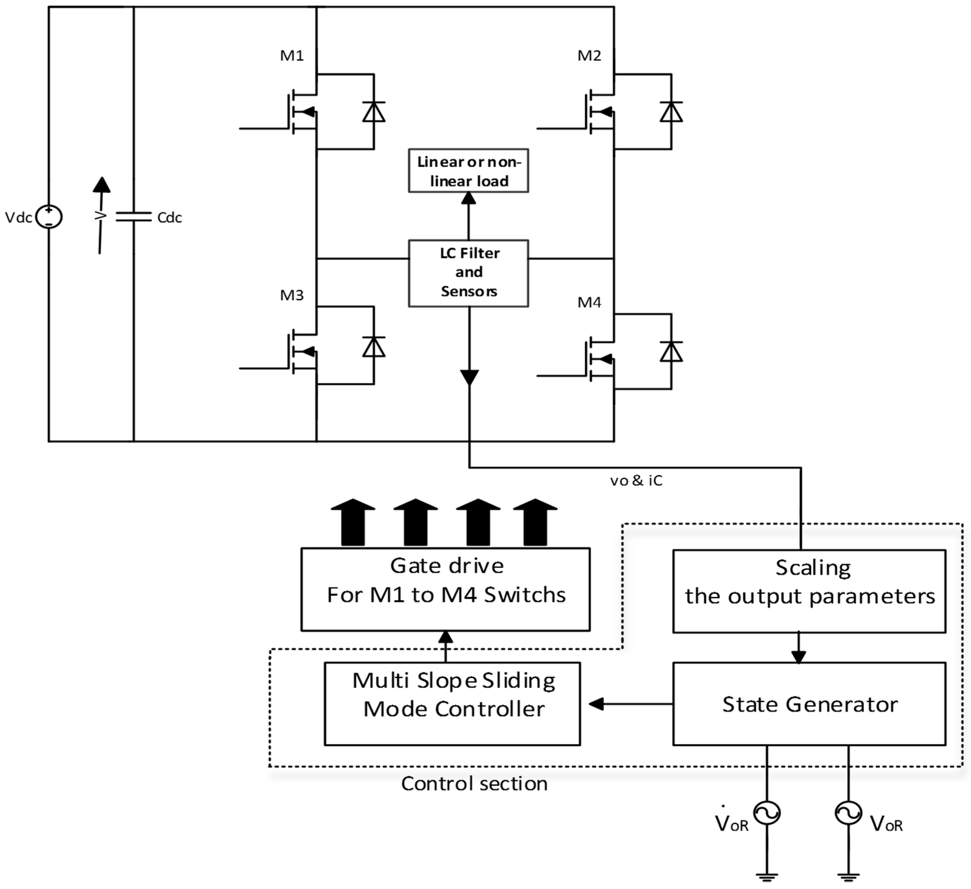
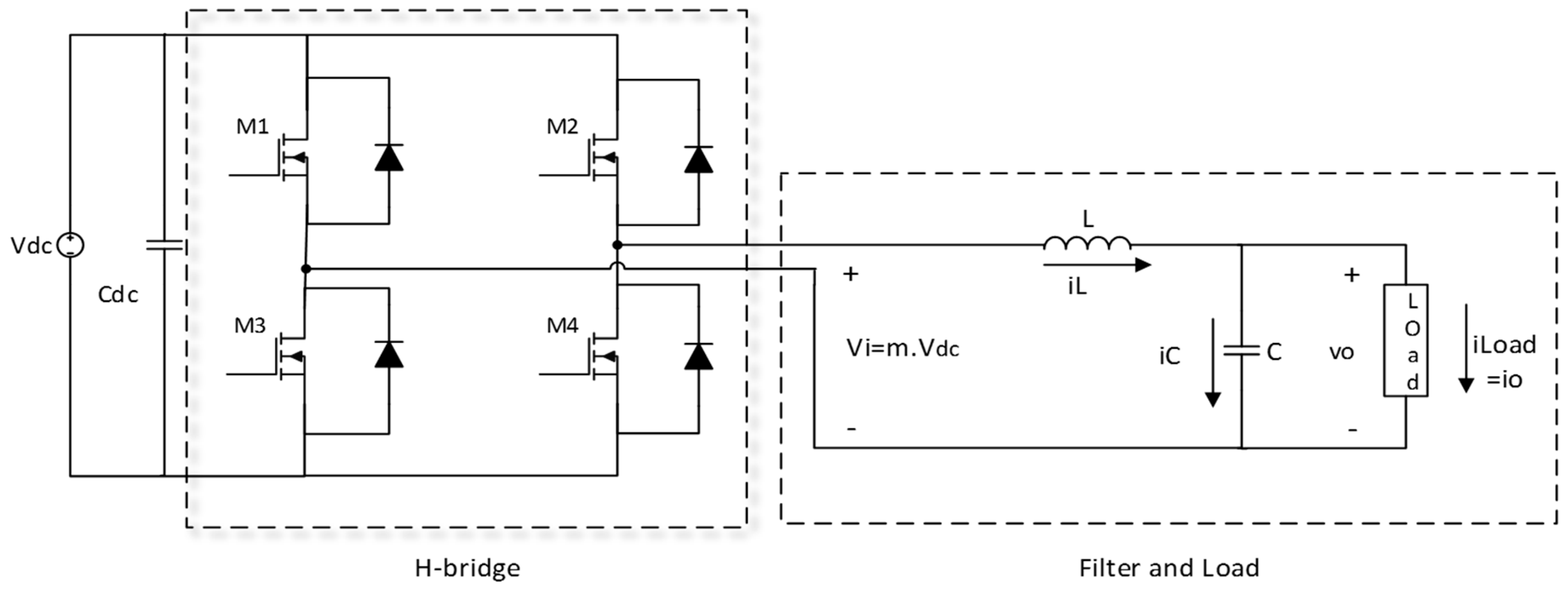
2. System Description

The main structure and power stage of the single-phase voltage source inverter (VSI) used in this research, as shown in Figure 1, consists of a switching part constructed by insulated-gate bipolar transistor (IGBT) or power MOSFET followed by 2nd or more order LC filter. Load in this case is located in parallel with the capacitor of the filter. In practice, to reduce the ESR effect and current ripple, several low ESR capacitors can be connected in parallel structure for the LC filter and it is worth mentioning that the small size of the filter capacitor is necessary and throughout this paper, the dc-link voltage is assumed to be constant, which can be realized by utilizing large capacitances at the dc-link of the inverter. The parameters of the inverter are given in

Table 1. Parameters for inverter model.

Parameter	Value
Fundamental Frequency, ω	2π50 $\raisebox{1ex}{$rad$}\!\left/ \!\raisebox{-1ex}{$s$}\right.$
Output Filter Inductance, L	250 µH
Output Filter Capacitance, C	100 µF
ESR of the filter Inductance and Capacitor, rL, rC	≈0
Dc-link voltage	460 V

. The equations describing the dynamics of the inverter can be obtained as:

$$v_L=L\frac{d{i}_L}{dt}=m{V}_{dc}-v_o$$

(1)

$$i_C=C\frac{d{v}_c}{dt}=i_L-i_{Load}$$

(2)

where m describes the control variable.

Considering low ESR capacitors are connected in parallel, the ESRs of the filter capacitor and inductor can be ignored. The state-space equation describing the operation of the system can be written in matrix form:

$$\left[\begin{array}{l}{\dot{v}}_o\\ {\dot{i}}_L\end{array}\right]=\left[\begin{array}{cc}0& \frac{1}{C}\\ -\frac{1}{L}& 0\end{array}\right]\left[\begin{array}{l}{v}_o\\ i_L\end{array}\right]+\left[\begin{array}{l}0\\ \frac{V_{dc}}{L}\end{array}\right]m+\left[\begin{array}{l}-\frac{1}{c}\\ 0\end{array}\right]i_{Load}$$

(3)

where $m\in \{-1,0,1\}$ is considered as the control input.

Based on Equations (1) and (2), the output voltage error [e(t)] and its derivative (rate of change of the output voltage error) are defined as:

$$e(t)=v_o-v_{oR}$$

(4)

$$x_1=e(t)$$

(5)

$$x_2={\dot{x}}_1={\dot{v}}_o-{\dot{v}}_{oR}$$

(6)

$${\dot{x}}_2=D(t)+(m{V}_{dc}-x_1){\mathsf{\omega }}_f^2$$

(7)

where dx₁/dt denotes the time derivative of x₁, ω_f = 1/(LC)^0.5, the time-varying term D(t) is considered as a disturbance, and $v_{oR}=V_{Rm}\sin (\mathsf{\omega }t)$ is the reference for output voltage. The disturbance term is defined as:

$$D(t)=-v_{oR}{\mathsf{\omega }}_f^2-\frac{1}{c}\frac{d(i_L-i_C)}{dt}-\frac{d{\dot{v}}_{oR}}{dt}$$

(8)

The behavior of the system can be expressed by the following state space controllable canonical form:

$$\left[\begin{array}{l}{\dot{x}}_1\\ {\dot{x}}_2\end{array}\right]=\left[\begin{array}{cc}0& 1\\ -{\mathsf{\omega }}_f^2& 0\end{array}\right]\left[\begin{array}{l}{x}_1\\ x_2\end{array}\right]+\left[\begin{array}{l}0\\ V_{dc}{\mathsf{\omega }}_f^2\end{array}\right]m+\left[\begin{array}{l}0\\ D(t)\end{array}\right]$$

(9)

Control of single-phase inverters under linear and non-linear loads using the sliding-mode method is well-improved research topic now. In order to achieve a desired control performance in different loading conditions, the controller should have the ability to ensure the low steady-state error in the presence of the inverter model uncertainties as well as other disturbances. In addition, to reduce the tracking error in moments of heavy loading, the controller must provide desired transient-states with negligible overshoots in the output voltage during the load current change. Therefore, the previous and single-slope method of sliding-mode control suffers from many problems such as single-slope and inflexible sliding surface, undesirable and poor transient-states in loading moments for sliding-mode controller with large slope of the surface, inability to achieve high-speed response and tracking accuracy simultaneously because of a significant reduction in existence regions for large slope of the surface.

3. Suggested Control Structure

In this section, the problems of conventional SMC will be explained briefly first; then, the novel non-linear function used to produce the multi-slope SMC (MSSMC) will be introduced; after that, its theoretical basis is developed and its coefficients adjustment is explained briefly; and, finally, based on a mathematical analysis, the improved performance of the proposed method will be confirmed. Figure 2 illustrates the suggested control structure, which consists of a MSSMC to regulate the instantaneous output voltage, state generator to provide the system states in order to use in proposed controller and a gate driver part, which is employed to trigger the switches of the VSI.

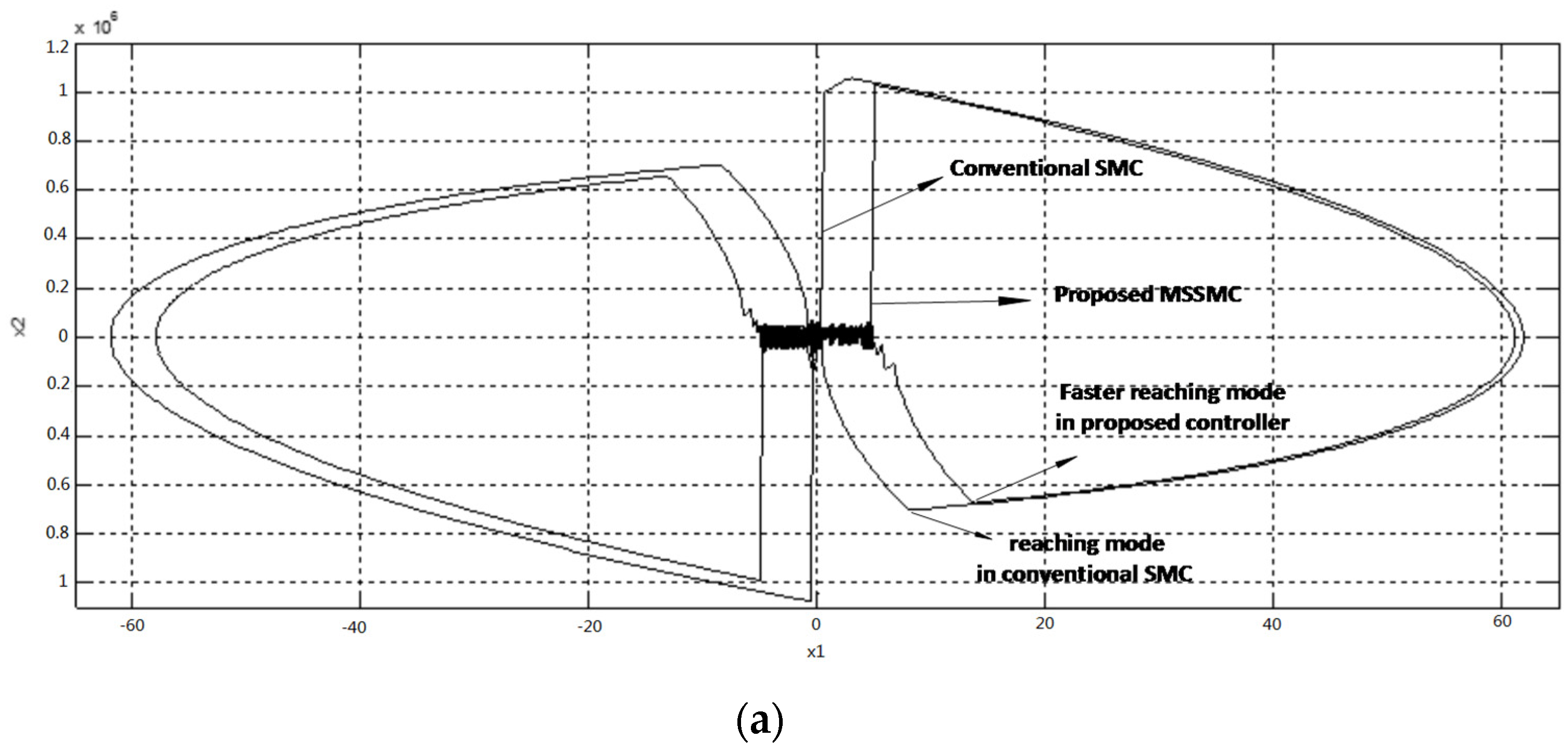
3.1. Conventional SMC Drawbacks

The conventional sliding-mode controller with single-slope sliding surface suffers from the following drawbacks. In the conventional sliding function, the integral term is not usually used to accumulate the existing steady-state errors. Even if the integral term is used, lack of flexibility in the integral term still exists for different values of the error. The principal reason behind this problem is the fixed-slope of the integral function for any values of error that can lead to wind-up the integral for different values of the tracking error.

As mentioned before, one of the most important drawbacks of the conventional sliding-mode controllers is single-slope and inflexible sliding surface. On the other hand, these controllers do not have the ability to achieve both high speed and desired transient-states in loading moments simultaneously. A surface with small slope leads to a slow response and low tracking accuracy and a surface with large slope leads to a poor transient-state during the load current change. A tradeoff between small and large slopes of the surface cannot realize both fast response and low THD response without any overshoots in output voltage simultaneously in moments of loading.

3.2. SMC Using Non-Linear Function

In order to overcome the conventional SMC drawbacks, to achieve a desired controller with high speed in reducing the tracking error in moments of loading, and to alleviate steady-state error under different types of loads without loss of the desired transient response, a flexible sliding surface composed of different terms of a special non-linear function is introduced. It should be noted here that each of these terms is made by a multi-slope non-linear function. Proposed sliding surface with an acceptable approximation consists of two general parts with different slopes, which are shown in Figure 3a as Part A and Part B. As can be obtained, when the error is generated by load current disturbance, for driving the system states to the sliding surface, a control low is applied to the system. In the sliding-mode, the state trajectory reaches Part B of the surface earlier and aligns the surface to Part A with high speed. Therefore, when the error value increases and output voltage drops because of the high current spikes of the load capacitance, the states trajectory hits Part B of the sliding surface first, which can lead to a faster reaching mode. It is important to know that, in the sliding-mode, the VSI will be robust and, by changing the slope of the surface, the system dynamics will also change.

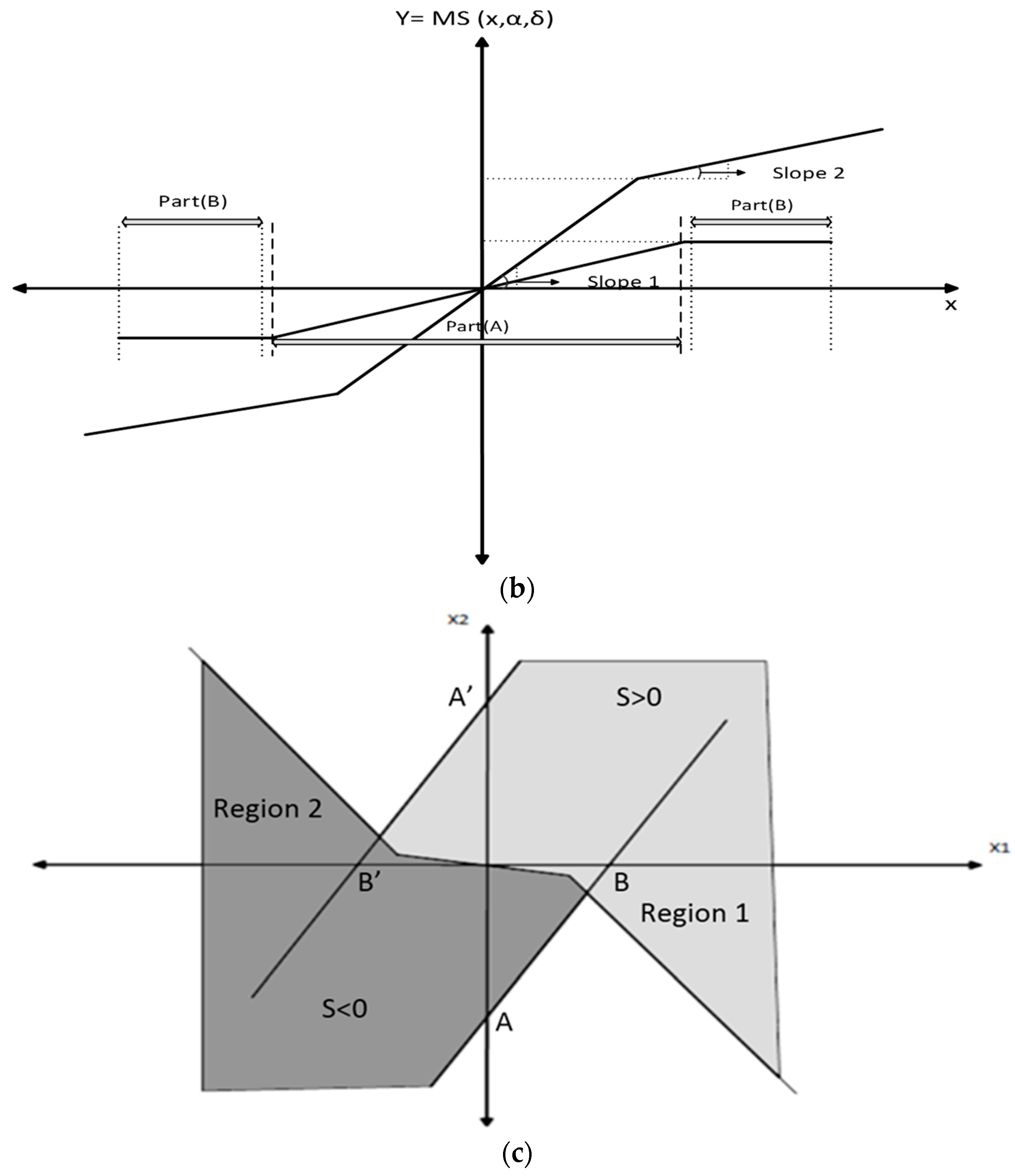
3.3. Multi-Slope (MS) Function

The Multi-Slope (MS) function can be described as:

$$Y=MS(x,\mathsf{\alpha },\mathsf{\delta })=({\mathsf{\alpha }}_{1}x+{\mathsf{\alpha }}_2\tan \mathrm{h}(\mathsf{\delta }x))$$

(10)

where α₁, α₂ and δ are adjustable coefficients of the function, which define the general form of the function and it is clear that MS function is a continuous and differentiable function. The variation of the slopes in Parts A and B and extent of these parts for different values of the multi-slope function coefficients (α₁, α₂, δ) are shown in Figure 3b. This clearly shows that the MS function includes two slopes and for small x values, the slope of Part A and for large value of x, the slope of Part B is more effective in this function.

In order to confirm the effectiveness of the MS function on the controller operation and to demonstrate the performance of the controller, the effectiveness of the proposed MSSMC has been described on a VSI loading behavior.

3.4. MS Function Coefficients Setting

The coefficients of the MS are α₁, α₂ and δ and to achieve a desired and fast dynamic response with almost negligible overshoot in the output voltage, these coefficients must be adjusted wisely. The tasks of these coefficients in the MS function structure are as follows:

(1)

δ coefficient: This coefficient adjusts the slope of Part A and should be positive (δ > 0). On the other hand, by changing this coefficient, the gain of the function will be changed for small error values.

(2)

α₁ coefficient: This coefficient is utilized in MS function to adjust the slope of Part B and its effect on slope of Part A is negligible. In principle, this coefficient is utilized to adjust the gain of the MS function for large values of the error.

(3)

α₂ coefficient: This coefficient adjusts the height of Part A. Therefore, by increasing this coefficient, the height of Part A will increase. It is worth mentioning that by increasing the value of this coefficient, low values of error in the input of the function creates more effect in the output of the function.

In general, the MS function is a non-linear function and use of this function in sliding function leads to yield a fast response with a desired transient-state without the need for any complex algorithm. On the other hand, if the coefficients of the MS function are adjusted wisely, a desired sliding surface will be generated, which leads to achieving a fast error convergence with a desired transient-state without any overshoots simultaneously.

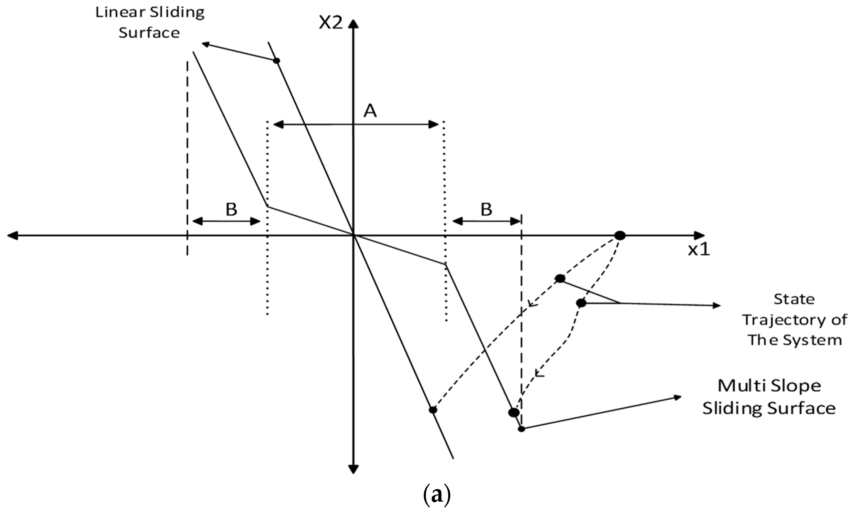
3.5. Sliding Surface and Stability Considerations

The sliding surface in MSSMC is composed of three MS functions and can be defined as:

$$S=MS(x_1,{\mathsf{\alpha }}_p,{\mathsf{\delta }}_p)+MS(x_2,{\mathsf{\alpha }}_d,{\mathsf{\delta }}_d)+{\displaystyle \int MS}(x_1,{\mathsf{\alpha }}_i,{\mathsf{\delta }}_i)dt$$

(11)

$$S=({\mathsf{\alpha }}_{p1}{x}_1+{\mathsf{\alpha }}_{p2}\tanh ({\mathsf{\delta }}_p{x}_1))+({\mathsf{\alpha }}_{d1}{x}_2+{\mathsf{\alpha }}_{d2}\tanh ({\mathsf{\delta }}_d{x}_2))+{\displaystyle \int ({\mathsf{\alpha }}_{i1}{x}_1+{\mathsf{\alpha }}_{i2}\tanh ({\mathsf{\delta }}_i{x}_1))}dt$$

(12)

In the sliding function, the integral term is added in order to reduce the steady-state error in output voltage and p, i, and d indexes represent the MS function in one of these three terms. When the sliding-mode is reached (S = 0), we have:

$${\mathsf{\alpha }}_{d1}{\dot{x}}_1+{\mathsf{\alpha }}_{d2}\tanh ({\mathsf{\delta }}_d{\dot{x}}_1)=-{\mathsf{\alpha }}_{p1}{x}_1-{\mathsf{\alpha }}_{p2}\tanh ({\mathsf{\delta }}_p{x}_1)-{\displaystyle \int ({\mathsf{\alpha }}_{i1}.x_1+{\mathsf{\alpha }}_{i2}\tanh ({\mathsf{\delta }}_i{x}_1))}dt$$

(13)

As can be seen, due to the structure of the MS function, the sliding surface is non-linear. It is worth mentioning that for proper performance of the controller, α_m1,2 must be positive where m can be p, i, and d. The existence condition must be satisfied for stability of reaching mode as:

$$S\stackrel{.}{S}<0$$

(14)

We consider the Lyapunov function as $V=0.5S^2$, and it is clear that for global stability $\dot{V}$ must be negative definite [41]. If this condition is satisfied, the state trajectory will be moved toward the surface and sliding can be preserved until the trajectory reached to the origin. By taking the time derivative of S, substituting Equations (6) and (7) into the resulting equation gives:

$$\begin{array}{l}\stackrel{.}{S}={\mathsf{\alpha }}_{p1}{x}_2+{\mathsf{\alpha }}_{p2}{x}_2{\mathsf{\delta }}_p{\mathrm{sech}}^2({\mathsf{\delta }}_p{x}_1)-{\mathsf{\alpha }}_{d1}{\mathsf{\omega }}_f^2{x}_1+{\mathsf{\alpha }}_{d1}{\mathsf{\omega }}_f^2{V}_{dc}m+D(t){\mathsf{\alpha }}_{d1}-{\mathsf{\alpha }}_{d2}{\mathsf{\delta }}_d{\mathsf{\omega }}_f^2{x}_1{\mathrm{sech}}^2({\mathsf{\delta }}_d{x}_2)+\\ {\mathsf{\alpha }}_{d2}{\mathsf{\delta }}_d{\mathsf{\omega }}_f^2{V}_{dc}m{\mathrm{sech}}^2({\mathsf{\delta }}_d{x}_2)+{\mathsf{\alpha }}_{d2}{\mathsf{\delta }}_{d}D(t){\mathrm{sech}}^2({\mathsf{\delta }}_d{x}_2)+{\mathsf{\alpha }}_{i1}{x}_1+{\mathsf{\alpha }}_{i2}\tanh ({\mathsf{\delta }}_i{x}_1)\end{array}$$

(15)

The above equation can be simplified as:

$$\stackrel{.}{S}={\mathsf{\epsilon }}_1(x_1)x_2-x_1({\mathsf{\epsilon }}_2(x_2){\mathsf{\omega }}_f^2-{\mathsf{\alpha }}_{i1})+{\mathsf{\epsilon }}_2(x_2)({\mathsf{\omega }}_f^2{V}_{dc}m+D(t))+{\mathsf{\alpha }}_{i2}\tanh ({\mathsf{\delta }}_i{x}_1)$$

(16)

The time derivative of the Lyapunov function is obtained as:

$$\dot{V}=S[{\mathsf{\epsilon }}_1(x_1)x_2-x_1({\mathsf{\epsilon }}_2(x_2){\mathsf{\omega }}_f^2-{\mathsf{\alpha }}_{i1})+{\mathsf{\epsilon }}_2(x_2)({\mathsf{\omega }}_f^2{V}_{dc}m+D(t))+{\mathsf{\alpha }}_{i2}\tanh ({\mathsf{\delta }}_i{x}_1)]$$

(17)

In Equation (17), ε₁(x₁) and ε₂(x₂) are defined as:

$${\mathsf{\epsilon }}_1(x_1)={\mathsf{\alpha }}_{p1}+{\mathsf{\delta }}_p{\mathsf{\alpha }}_{p2}{\mathrm{sech}}^2(x_1{\mathsf{\delta }}_p)$$

(18)

$${\mathsf{\epsilon }}_2(x_2)={\mathsf{\alpha }}_{d1}+{\mathsf{\delta }}_d{\mathsf{\alpha }}_{d2}{\mathrm{sech}}^2(x_2{\mathsf{\delta }}_d)$$

(19)

Substitution of m = −sign(s) into Equation (17) yields:

$$\dot{V}(t)=S\left[{\mathsf{\epsilon }}_1(x_1)x_2-x_1({\mathsf{\epsilon }}_2(x_2){\mathsf{\omega }}_f^2-{\mathsf{\alpha }}_{i1})-{\mathsf{\epsilon }}_2(x_2)({\mathsf{\omega }}_f^2{V}_{dc}sign(s)-D(t))+{\mathsf{\alpha }}_{i2}\tanh ({\mathsf{\delta }}_i{x}_1)\right]$$

(20)

$$\dot{V}(t)=\left|S\right|\left\{sign(s)\left[{\mathsf{\epsilon }}_1(x_1)x_2-x_1({\mathsf{\epsilon }}_2(x_2){\mathsf{\omega }}_f^2-{\mathsf{\alpha }}_{i1})+{\mathsf{\epsilon }}_2(x_2)D(t)+{\mathsf{\alpha }}_{i2}\tanh ({\mathsf{\delta }}_i{x}_1)\right]-{\mathsf{\epsilon }}_2(x_2){\mathsf{\omega }}_f^2{V}_{dc}\right\}$$

(21)

It is clear that $\dot{V}(t)<0$ if:

$$sign(s)\left[{\mathsf{\epsilon }}_1(x_1)x_2-x_1({\mathsf{\epsilon }}_2(x_2){\mathsf{\omega }}_f^2-{\mathsf{\alpha }}_{i1})+{\mathsf{\epsilon }}_2(x_2)D(t)+{\mathsf{\alpha }}_{i2}\tanh ({\mathsf{\delta }}_i{x}_1)\right]<{\mathsf{\epsilon }}_2(x_2){\mathsf{\omega }}_f^2{V}_{dc}$$

(22)

The following inequalities can be obtained from Equation (22):

$$\begin{array}{r}{A}_1=-x_2+x_1(\frac{{\mathsf{\epsilon }}_2(x_2){\mathsf{\omega }}_f^2-{\mathsf{\alpha }}_{i1}}{{\mathsf{\epsilon }}_1(x_1)})-\frac{{\mathsf{\epsilon }}_2(x_2)}{{\mathsf{\epsilon }}_1(x_1)}D(t)-\frac{{\mathsf{\alpha }}_{i2}}{{\mathsf{\epsilon }}_1(x_1)}\tanh ({\mathsf{\delta }}_i{x}_1)-\frac{{\mathsf{\epsilon }}_2(x_2)}{{\mathsf{\epsilon }}_1(x_1)}{\mathsf{\omega }}_f^2\\ V_{dc}>0forS<0\end{array}$$

(23)

$$\begin{array}{r}{A}_2=-x_2+x_1(\frac{{\mathsf{\epsilon }}_2(x_2){\mathsf{\omega }}_f^2-{\mathsf{\alpha }}_{i1}}{{\mathsf{\epsilon }}_1(x_1)})-\frac{{\mathsf{\epsilon }}_2(x_2)}{{\mathsf{\epsilon }}_1(x_1)}D(t)-\frac{{\mathsf{\alpha }}_{i2}}{{\mathsf{\epsilon }}_1(x_1)}\tanh ({\mathsf{\delta }}_i{x}_1)+\frac{{\mathsf{\epsilon }}_2(x_2)}{{\mathsf{\epsilon }}_1(x_1)}{\mathsf{\omega }}_f^2\\ V_{dc}<0forS>0\end{array}$$

(24)

Figure 3c illustrates the regions of existence of the sliding-mode. It is clear from Equations (23) and (24) that A₁ = 0 and A₂ = 0 are two lines in the x₁-x₂ plane for the practical values of the inverter parameters. Note that the slopes of these lines are equal which means that these lines are parallel with each other. This slope can be obtained as:

$$s_{L1}=s_{L2}\cong \frac{({\mathsf{\epsilon }}_2(0){\mathsf{\omega }}_f^2+{\mathsf{\alpha }}_{i1}){\mathsf{\epsilon }}_2(x_2)}{{\mathsf{\epsilon }}_1(0){\mathsf{\epsilon }}_2(0)}\cong \frac{{\mathsf{\epsilon }}_2(x_2){\mathsf{\omega }}_f^2}{{\mathsf{\epsilon }}_1(0)}$$

(25)

The intersection points of these lines with x₁ and x₂ axes can be obtained from Equations (26)–(29).

$$x_2=-\frac{{\mathsf{\epsilon }}_2(D(t)+{\mathsf{\omega }}_f^2{V}_{dc})}{{\mathsf{\epsilon }}_1(0)}\to A_1=0with{x}_2-axis$$

(26)

$$x_2=-\frac{{\mathsf{\epsilon }}_2(D(t)-{\mathsf{\omega }}_f^2{V}_{dc})}{{\mathsf{\epsilon }}_1(0)}\to A_2=0with{x}_2-axis$$

(27)

$$x_1=\frac{{\mathsf{\epsilon }}_2(0)(D(t)+{\mathsf{\omega }}_f^2{V}_{dc})+{\mathsf{\alpha }}_{i2}\tanh ({\mathsf{\delta }}_i{x}_1)}{{\mathsf{\epsilon }}_2(0){\mathsf{\omega }}_f^2-{\mathsf{\alpha }}_{i1}}\to A_1=0with{x}_1-axis$$

(28)

$$x_1=\frac{{\mathsf{\epsilon }}_2(0)(D(t)-{\mathsf{\omega }}_f^2{V}_{dc})+{\mathsf{\alpha }}_{i2}\tanh ({\mathsf{\delta }}_i{x}_1)}{{\mathsf{\epsilon }}_2(0){\mathsf{\omega }}_f^2-{\mathsf{\alpha }}_{i1}}\to A_2=0with{x}_1-axis$$

(29)

If the following condition holds:

$$\mathsf{\omega }{}_f^2{\mathsf{\epsilon }}_2(0)>>{\mathsf{\alpha }}_{i2},{\mathsf{\alpha }}_{i1}$$

(30)

Equations (28) and (29) can be approximated by:

$$x_1\cong \frac{(k_1(t))}{{\mathsf{\omega }}_f^2}\to A_1=0with{x}_1-axis$$

(31)

$$x_1\cong \frac{(k_2(t))}{{\mathsf{\omega }}_f^2}\to A_2=0with{x}_1-axis$$

(32)

where k₁(t) and k₂(t) are defined as:

$$k_1(t)=D(t)+{\mathsf{\omega }}_f^2{V}_{dc}$$

(33)

$$k_2(t)=D(t)-{\mathsf{\omega }}_f^2{V}_{dc}$$

(34)

Due to stability considerations, the existence regions should be kept as large as possible. As can be obtained from Equations (25)–(29), if ε₁(0) increases to achieve a faster response, this large value of ε₁(0) causes a reduction in sliding-mode existing region which can lead to an overshoot in output voltage. It is clear that for very large value of ε₁(0), instability can be occurred in the system because of the excessive reduction of the existence regions. In order to increase the sliding-mode existing regions and to reduce the overshoots in output voltage for large value of ε₁(0), it is clear that ε₂(0) can be adjusted wisely so that the high speed response is yielded and the overshoot is eliminated from the output voltage. Therefore, the distance between the intersection points of the x₂-axis and origin will be increased. In most cases, the following condition holds:

$${\mathsf{\epsilon }}_2(0){\mathsf{\omega }}_f^2+{\mathsf{\alpha }}_{i1}>>\mathsf{\alpha }{i}_2$$

(35)

It is clear that the system become unstable with very large ε₁(x₁)/ε₂(x₂) value. In most cases, α_i1 and α_i2 are chosen so that the following condition holds:

$${\mathsf{\epsilon }}_1(x_1)>>(x_1{\mathsf{\alpha }}_{i1}+{\mathsf{\alpha }}_{i2}\tanh ({\mathsf{\delta }}_i{x}_1))$$

(36)

According to Equation (36) combined with Equations (23) and (24), we obtain:

$${x_2}^{-1}(x_1{\mathsf{\omega }}_f^2-D(t)+{\mathsf{\omega }}_f^2{V}_{dc})>\frac{{\mathsf{\epsilon }}_1(x_1)}{{\mathsf{\epsilon }}_2(x_2)}>{x_2}^{-1}(x_1{\mathsf{\omega }}_f^2-D(t)-{\mathsf{\omega }}_f^2{V}_{dc})$$

(37)

An upper bound of ε₁(x₁)/ε₂(x₂) can be determined by:

$${x_2}^{-1}(x_1{\mathsf{\omega }}_f^2-k_2(t))>\frac{{\mathsf{\epsilon }}_1(x_1)}{{\mathsf{\epsilon }}_2(x_2)}$$

(38)

Clearly, the upper bound does not depend on one parameter and has a flexible and adjustable structure, which can lead to a fast response without any overshoots.

4. Simulation Results

In this section, the simulation results of an inverter controlled by proposed multi-slope sliding-mode controller under linear and non-linear loads have been evaluated. Due to limited switching frequency of an inverter, the direct implementation of m = −sign(s) is not possible for a VSI in practice. In order to prevent chattering, operating frequency has to be limited to a finite form by replacing a suitable hysteresis function instead of sign function. It is worth mentioning that the simulations are carried out using the Sim-Power-Systems toolbox of Simulink. Figure 4a shows the output voltages for an inverter controlled by proposed MSSMC and a fast controller with high performance proposed in [42]. As can be obtained, both of them are adjusted to generate high speed response with a very low voltage ripple in output voltage. It is clear that MSSMC leads to an output voltage without any overshoot and Figure 4b shows a larger view of this figure in the loading moment. The simulation results of the proposed controller are obtained when the controller coefficients are chosen as: α_p1 = 3 × 10⁶, α_p2 = 6 × 10⁵, α_d1 = 30, α_d2 = 7.2 × 10⁶, α_i1 = 2 × 10⁵, α_i2 = 6 × 10⁵, δ_p = 4000, δ_d = 101,000, and δ_i = 6 × 10³.

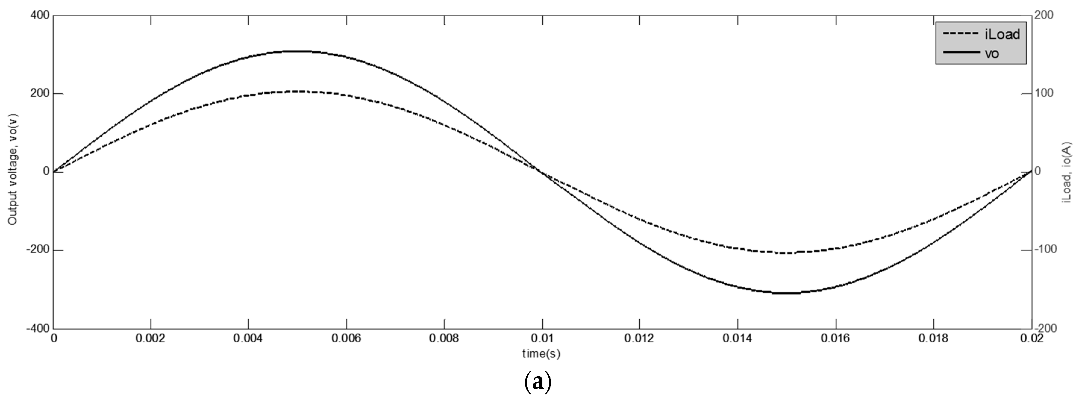
4.1. Resistive Load (R = 3 Ω)

By utilizing these coefficients, the system response is fast with a negligible overshoot. Figure 5a shows the simulated waveforms of output voltage and load current for a resistive load (R = 3 Ω). Figure 5b,c shows the spectrum of the output voltage for this case. It is clear that the magnitude of the output voltage fundamental component is much larger than the other components and, as can be seen, the regulation of the output voltage is preserved. The output voltage THD and the load current THD are obtained as 0.41% and the output PF is obtained as 0.99 for this case.

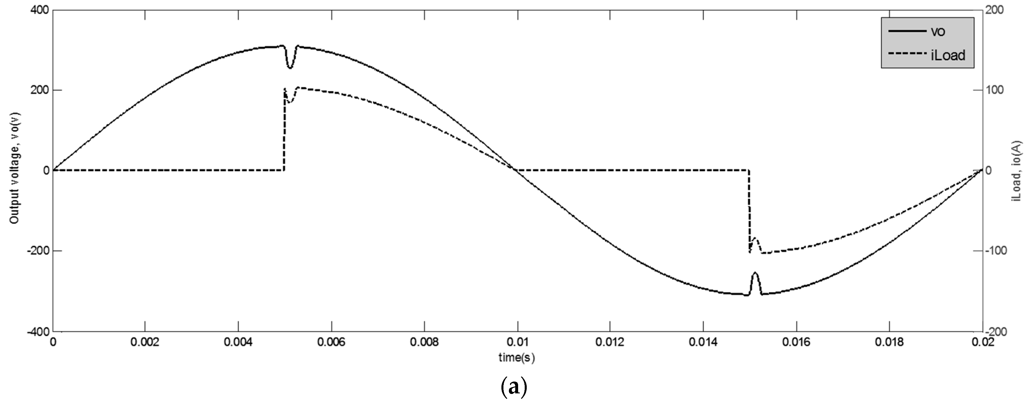
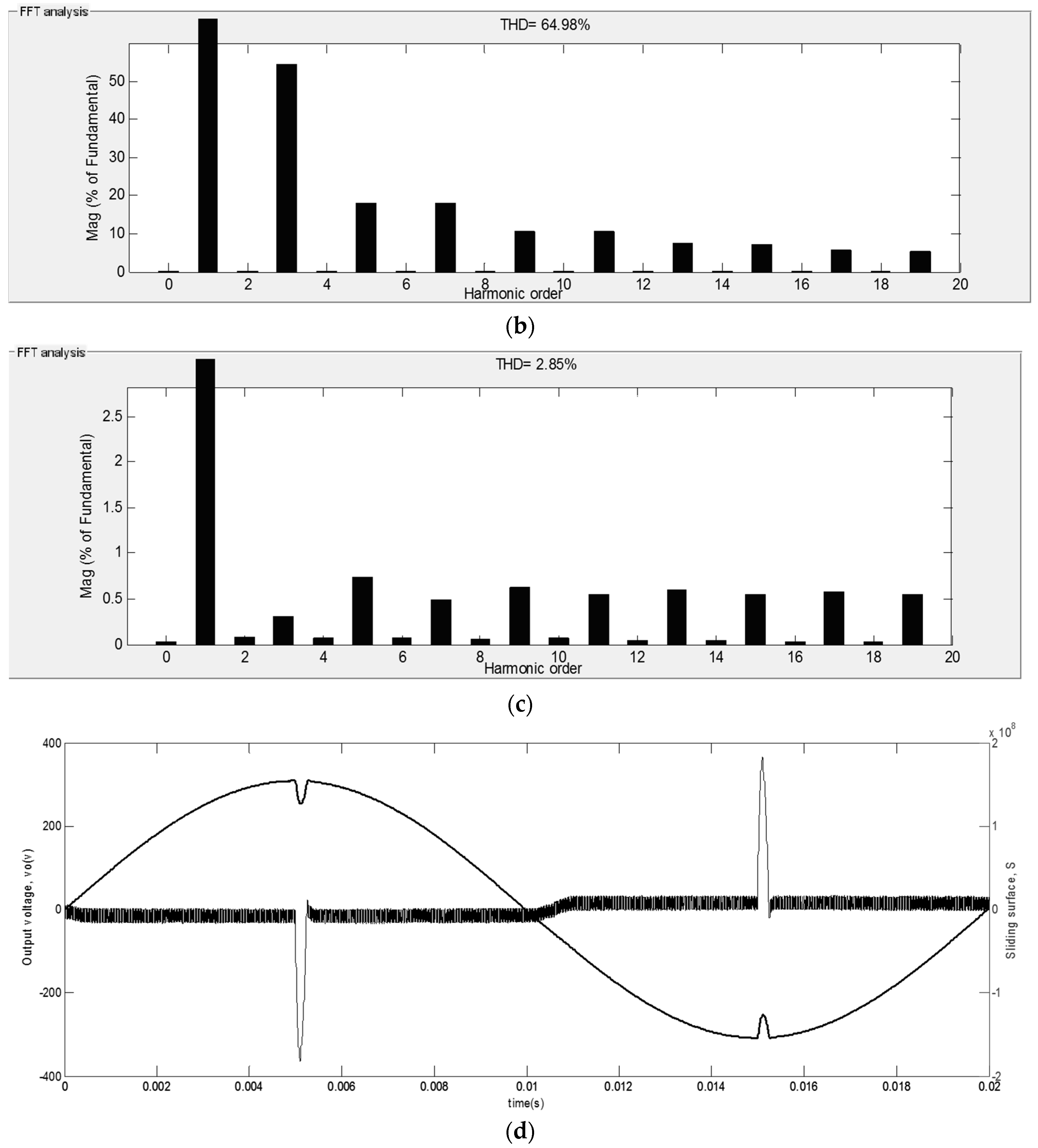
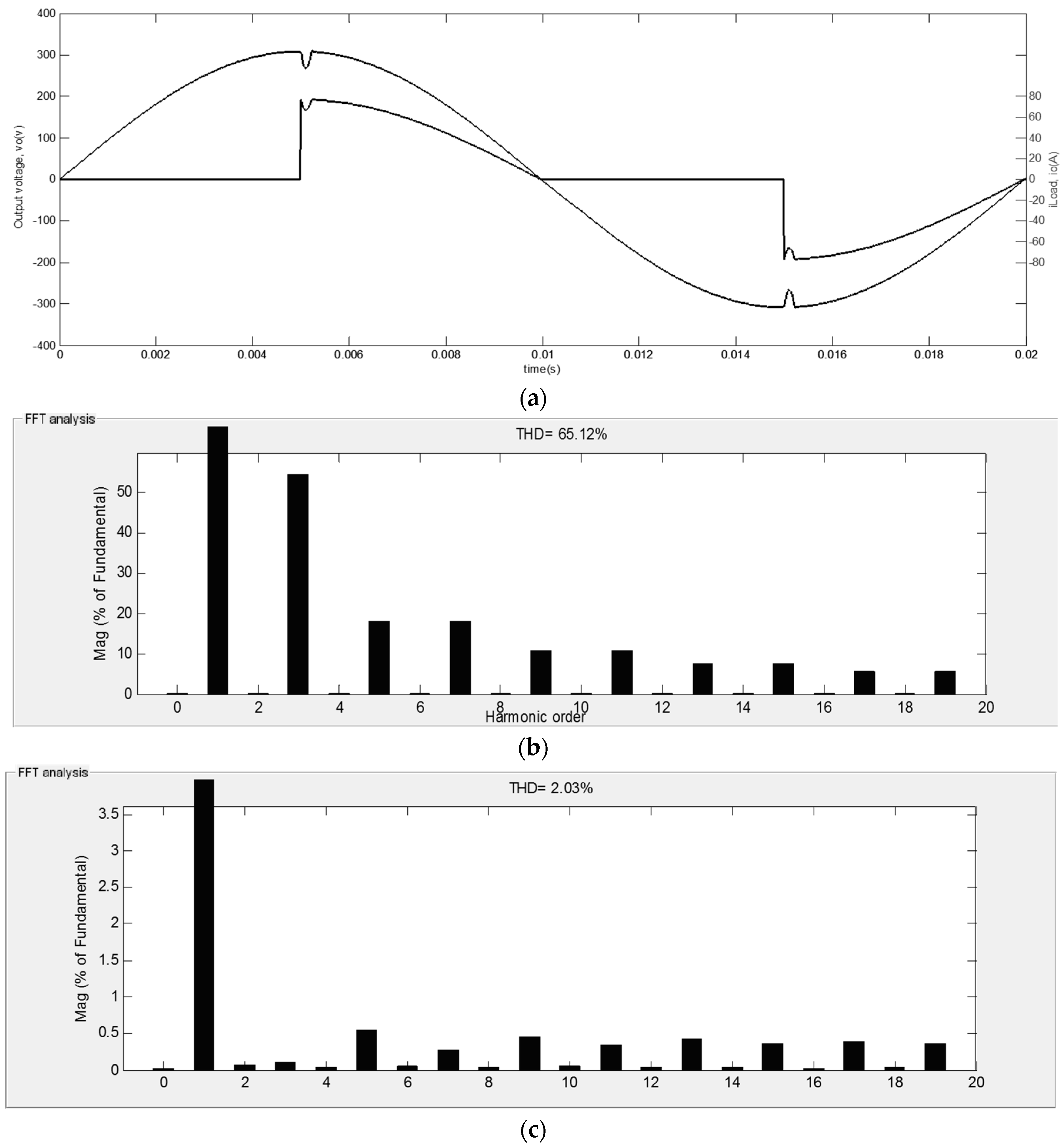
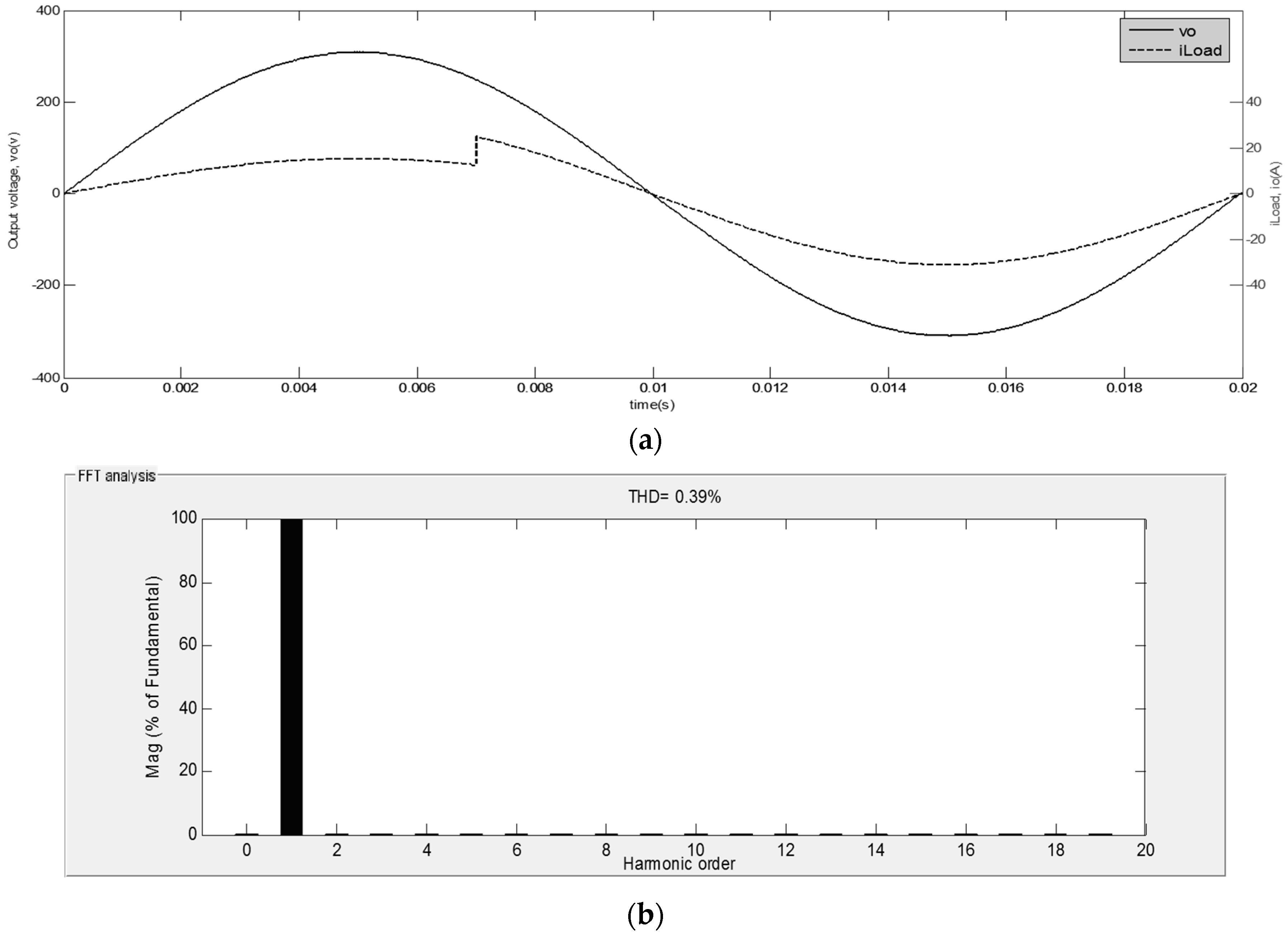
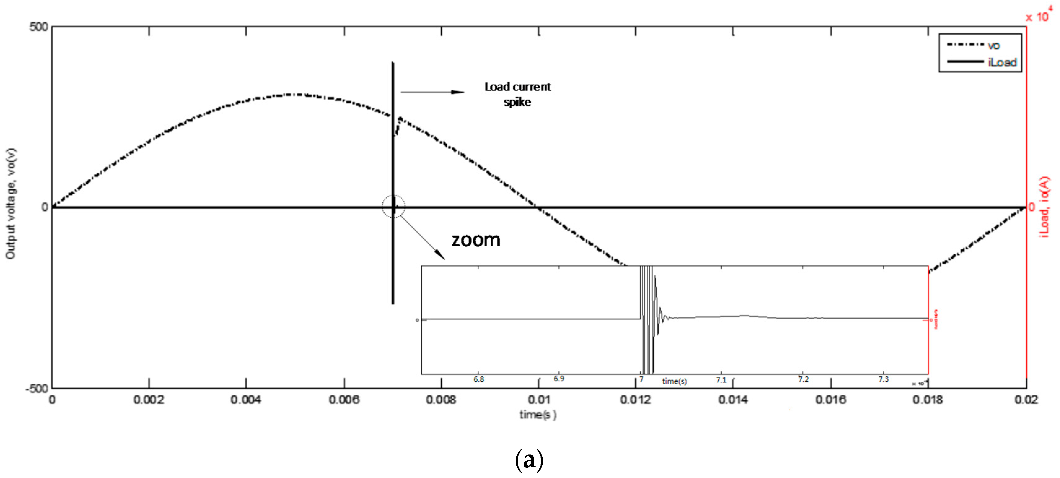
4.2. Non-Linear TRIAC-Controlled Resistive Load (R = 3 Ω)

Figure 6a depicts the output voltage and load current waveforms for a non-linear TRIAC-controlled resistive load (R = 3 Ω). The load current changes at the peak of the output voltage and, as can be observed, the output voltage regulation is fully preserved and the tracking error reduces with high speed and, as can be obtained from Figure 6b,c, the output voltage THD is limited to under 2.85%. The load current THD is obtained as 64.98% and the output PF is obtained as 0.84 for this load. Figure 6d shows the output voltage and the sliding function for a non-linear TRIAC-controlled resistive load case. Because of the structure of m, the sliding function varies between zero and negative or positive value in positive and negative cycles of the output voltage, respectively.

4.3. Non-Linear TRIAC-Controlled Resistive Load (R = 4 Ω)

To demonstrate the desired performance of the proposed controller for different levels of power, the output voltage and load current for a TRIAC-controlled resistive load (R = 4 Ω) are shown in Figure 7a and the spectrum of the load current and the output voltage for this load are illustrated in Figure 7b,c, respectively. From these plots, it can be concluded that the controller performance is as desired, regulation of the output voltage is preserved and the THD of the output voltage for this load case is 2.03%. It is worth noting that the load current THD for this load case is 65.12% and the output PF is obtained as 0.83.

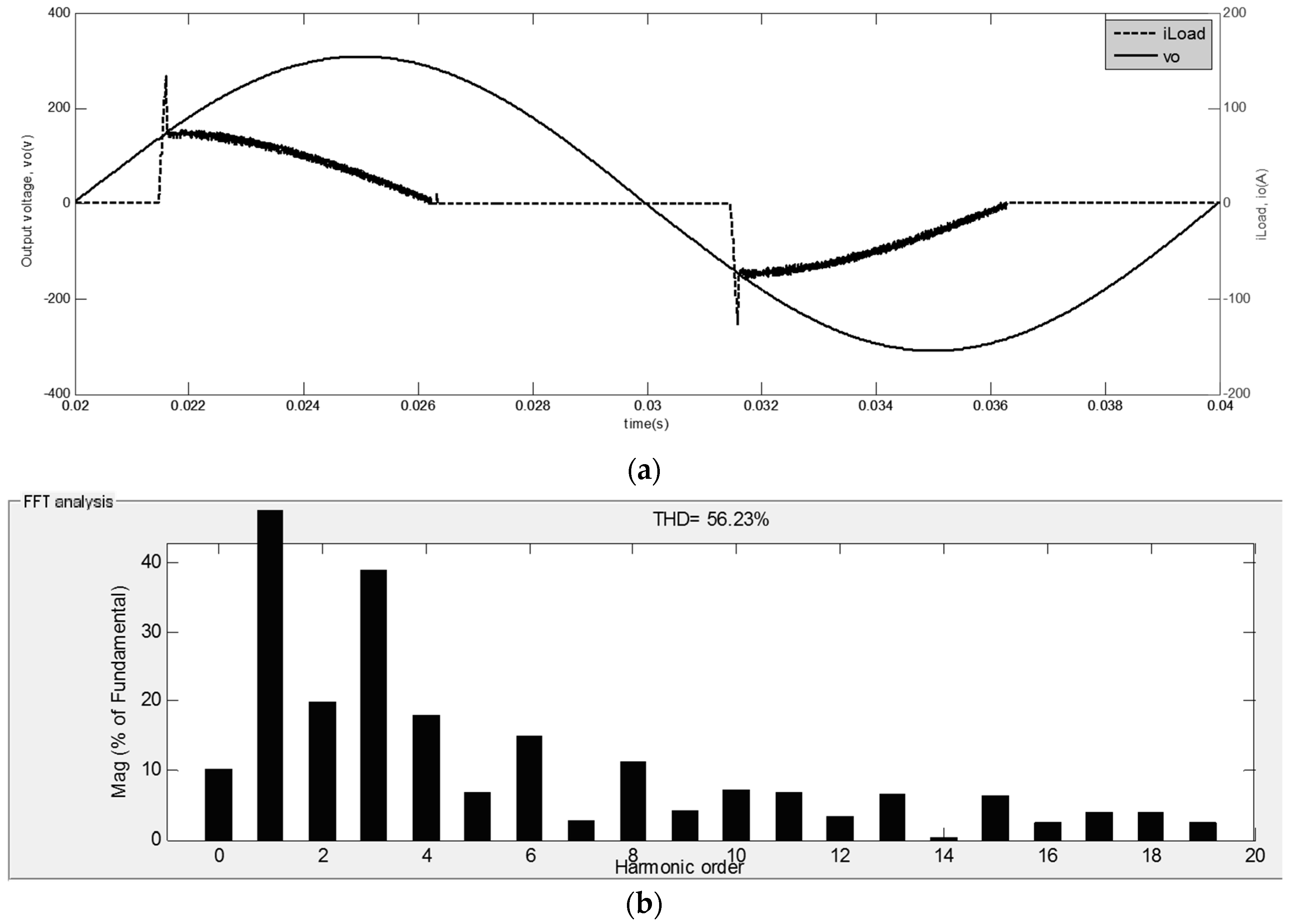
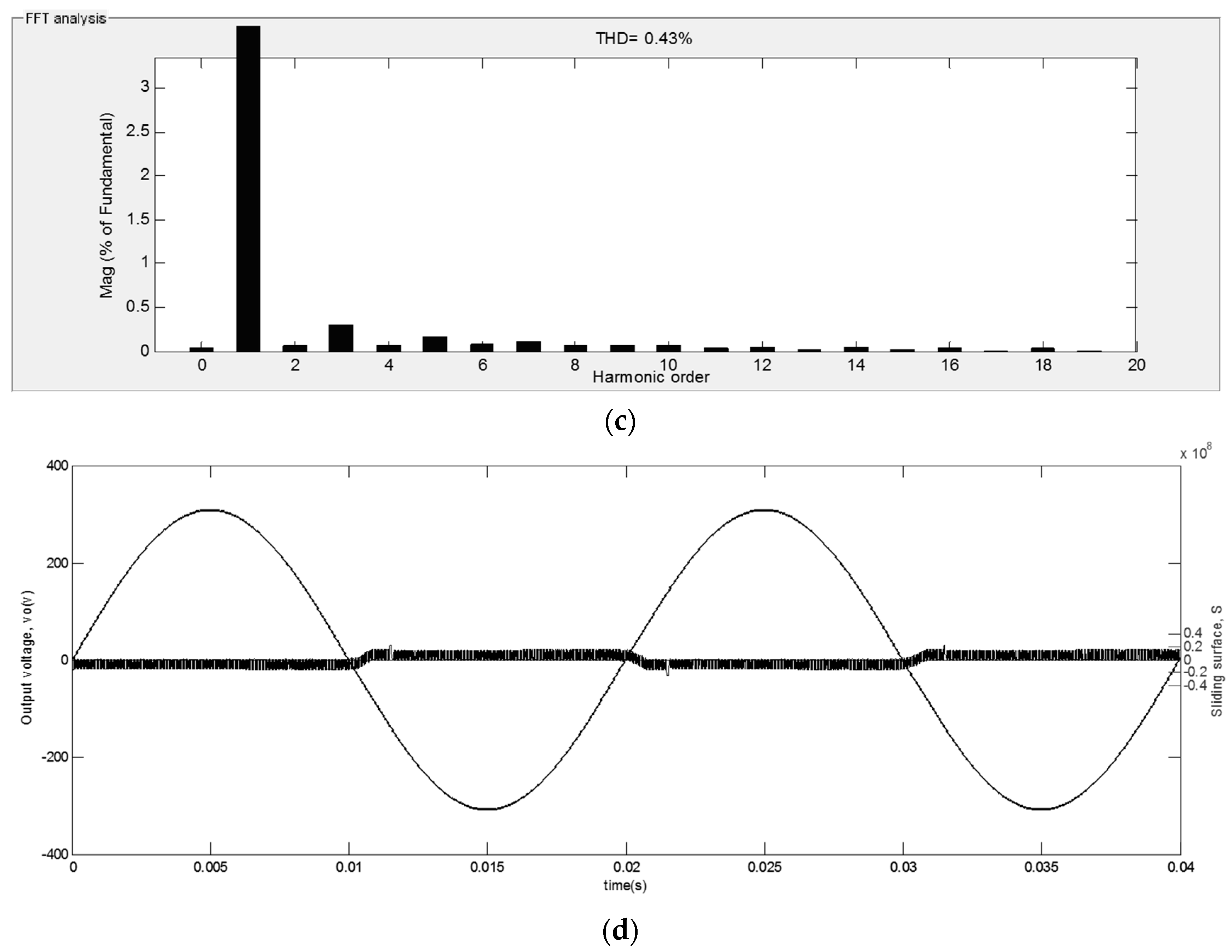
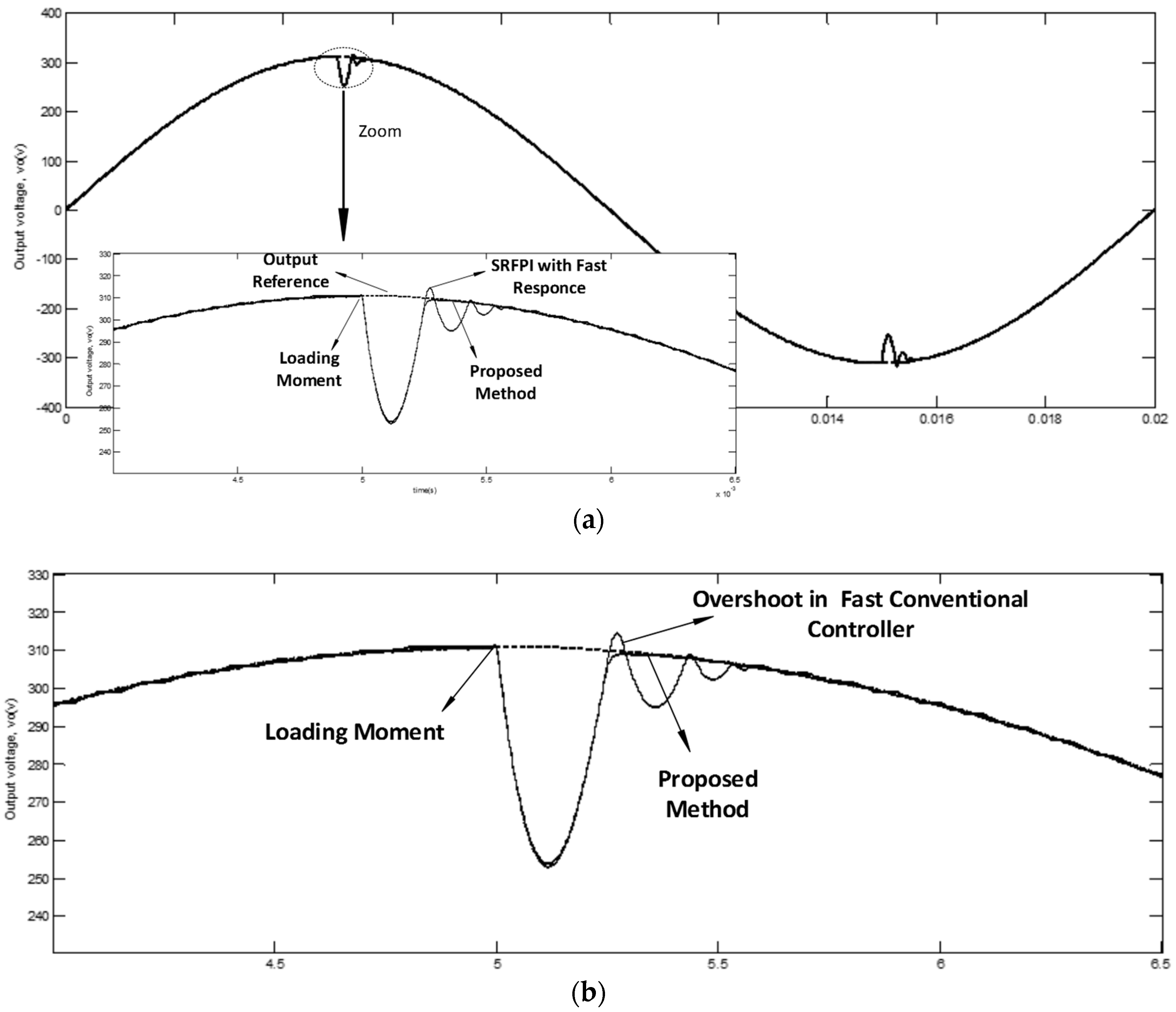
4.4. Dynamic Change in the Load Resistance

Figure 8a shows that the output voltage remaining constant when a sudden change occurs in the load resistance (at t = 7 ms) and confirms that the MSSMC has good robustness against the load disturbances. The spectrum of the output voltage is shown in Figure 8b and, as can be seen, the THD of the output voltage for this dynamic change in load is 0.39%. It is worth noting that the load current THD for this load case is 21.5% and the output PF is obtained as 0.98.

4.5. Load Type Change

The output voltage and the load current waveforms of the converter when the load suddenly changes from a resistive type to a capacitive-resistive type are shown in Figure 9a. As can be obtained, when the capacitive-resistive load is suddenly applied to the output of the converter, due to the large current spikes of the capacitor, the load current is highly distorted. Nevertheless, the output voltage is sinusoidal in shape and, as can be seen from Figure 9b, output the THD of the output voltage is 1.46%.

4.6. Rectifier Load

Figure 10a shows the output voltage and the load current for a bridge-rectifier having 10 Ω in parallel with a 700 µF at the output of the bridge. The spectrum of the load current and the output voltage is shown in Figure 10b,c, respectively, and, in this case, the THD of the output voltage is obtained as 0.43%, the load current THD is obtained as 56.23% and the output PF is obtained as 0.86. The output voltage and the sliding function for this bridge-rectifier load is shown in Figure 10d.

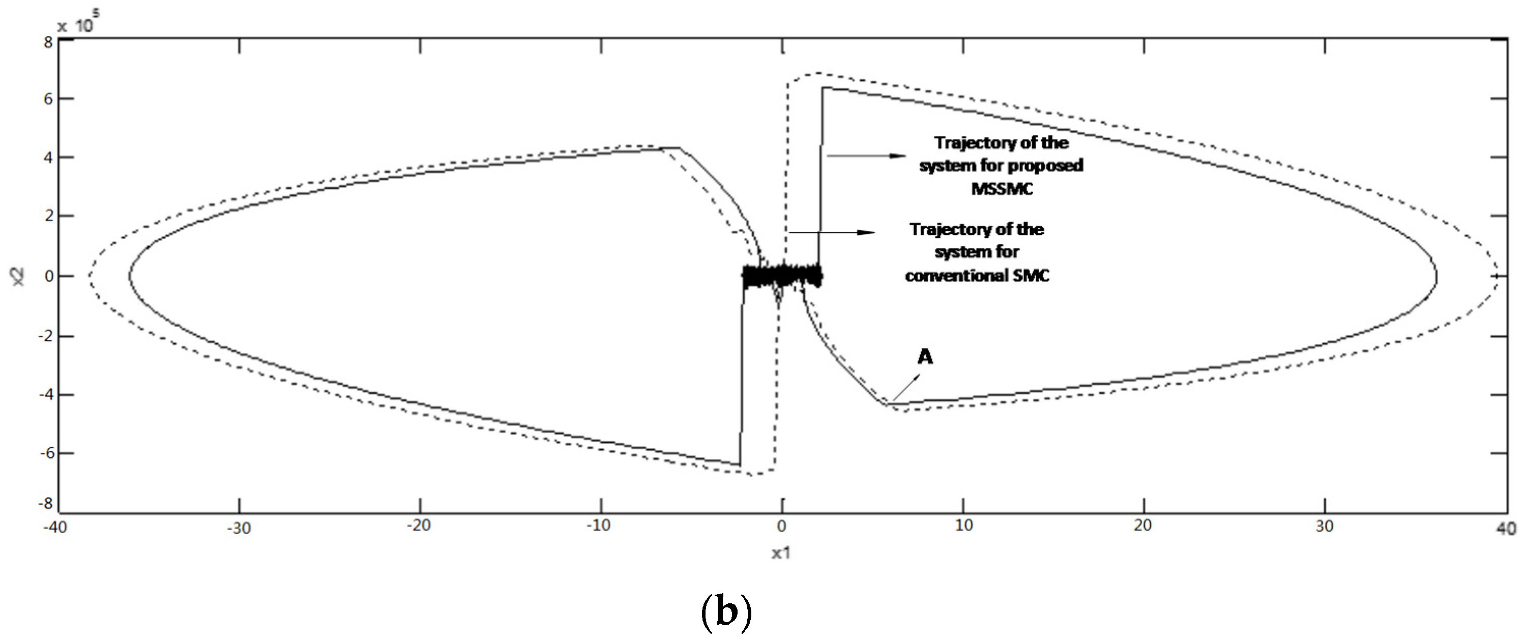
4.7. State Trajectories

Figure 11a depicts the state trajectories of the inverter controlled with proposed and conventional sliding-mode controller. It is obvious that the response of the output voltage can be made faster and the output voltage drop (x₁ value) can be reduced using the proposed MSSMC method. When the current disturbance occurs and the trajectory moves toward the surface, the reaching mode can be reached faster than the conventional SMC because of the improved surface structure. Figure 11b shows a comparison between the proposed and conventional SMC with the same reaching time. As can be obtained, in both cases, the trajectories reach each other at Point A, but, as can be seen, the drop of the output voltage for the inverter, which is controlled by proposed method, is lower than the conventional SMC.

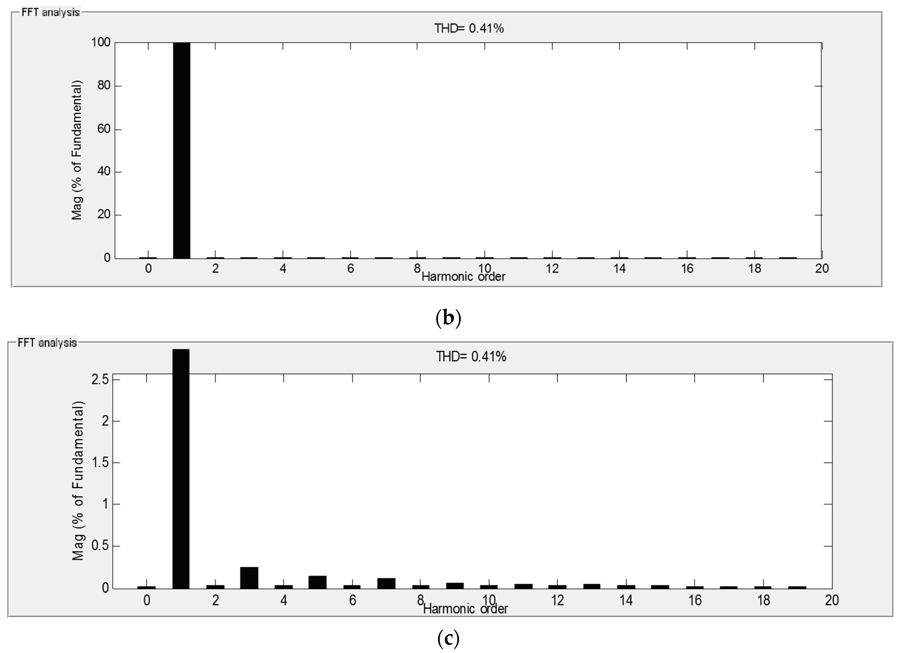
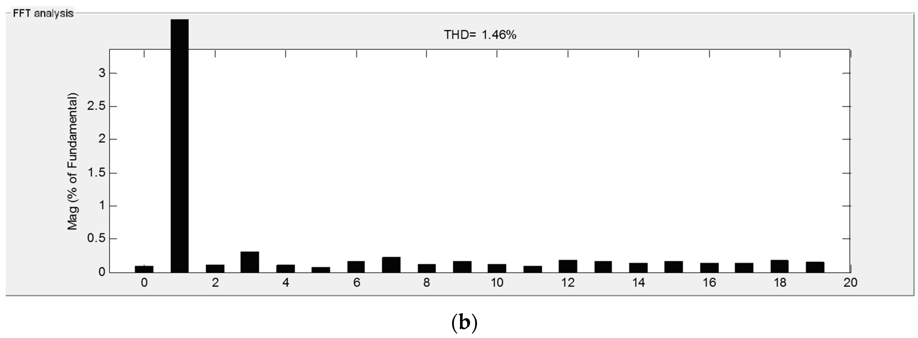
4.8. Comparative THD

The quality of inverter can be evaluated by THD value of output voltage and characteristics of transient response. The power quality depends on the choice of inverter control methods. THD is one important index to evaluate the performance of the inverters. The simulation results of proposed MSSMC controller in comparison with conventional SMC and a fast controller [42] are evaluated in the same inverter topology and loading conditions for non-linear load case.

Table 2. THD (total harmonic distortion) and harmonics of the output voltage for three control methods.

Comparison Category	Proposed Method in [42] kp = 25, ki = 60, k = 30	Proposed MSSMC	Single Slope SMC (s = λx1 + x2), λ = 75,000
THD (%) for non-linear load case	3	2.85	3.22
Output Voltage Fundamental (v)	308.4	306.2	308.6
2nd harmonic (% of fundamental)	0.036	0.08	0.005
3rd harmonic (% of fundamental)	0.63	0.3	0.69
4th harmonic (% of fundamental)	0.042	0.078	0.001
5th harmonic (% of fundamental)	0.75	0.74	0.71
Robustness	Good	Very good	Very good

summarizes the output voltage harmonic analysis in three methods for the TRIAC-controlled resistive load case. As can be obtained, three techniques can supply different load types with very small THD in generated voltage but the proposed technique produced an output voltage with lower harmonic contents than the output voltage produced by the conventional SMC and fast controller under the non-linear load.

5. Conclusions

In order to achieve an accurate and desired performance of single-phase sinusoidal inverter under different load types, a new approach to the sliding-mode controller is introduced in this paper. The proposed structure of sliding-mode control has not been investigated yet for inverters and switching converters. In this controller, by using a non-linear multi-slope function (MS), a multi-slope sliding surface is made consisting of two parts with different slopes. The slope of the surface in each part can be changed by setting the coefficients of the multi-slope function. It is shown that, in this approach, the speed of the controller to reduce the tracking error in moments of heavy loading can be increased and fast transient-states can be obtained without any overshoot. Therefore, the proposed approach leads to achieving a high-speed response with desired transient-states when the load current changes and under a highly non-linear load. Finally, the performance of the proposed control strategy has been confirmed through simulations.

References

1. Geisa, J.M.; Rajaram, M. Selective elimination of harmonic contents in an uninterruptible power supply: An enhanced adaptive hybrid technique. IET Power Electron. 2012, 5, 1527–1534. [Google Scholar] [CrossRef]
2. Roy, S.; Umanand, L. Magnetic arm-switch-based three-phase series-shunt compensated quality ac power supply. IET Electr. Power Appl. 2012, 6, 91–100. [Google Scholar] [CrossRef]
3. Faiz, J.; Shahgholian, G.; Mahdavian, M. Analysis and simulation of a three-phase UPS inverter with output multiple-filter. Armen. J. Phys. 2009, 2, 317–325. [Google Scholar]
4. Tian, J.; Chen, Q.; Xie, B. Series hybrid active power filter based on controllable harmonic impedance. IET Power Electron. 2012, 5, 142–148. [Google Scholar] [CrossRef]
5. Massoud, A.M.; Finney, S.J.; Cruden, A.; Williams, B.W. Mapped phase-shifted space vector modulation for multi-level voltage-source inverters. IET Electr. Power Appl. 2007, 1, 622–636. [Google Scholar] [CrossRef]
6. Sekhar, K.R.; Srinivas, S. Discontinuous decoupled PWMs for reduced current ripple in a dual two-level inverter fed open-end winding induction motor drive. IEEE Trans. Power Electron. 2012, 28, 2493–2502. [Google Scholar] [CrossRef]
7. Chen, Y.; Liu, T.H.; Cuong, N.M. Implementation of sensorless DC-link capacitorless inverter-based interior permanent magnet synchronous motor drive via measuring switching-state current ripples. IET Electric Power Appl. 2016, 10, 197–207. [Google Scholar] [CrossRef]
8. Lin, B.R.; Dong, J.Y. New zero-voltage switching DC-DC converter for renewable energy conversion systems. IET Power Electron. 2012, 5, 393–400. [Google Scholar] [CrossRef]
9. Shahgholian, G.; Khani, K.; Moazzami, M. Frequency control in autanamous microgrid in the presence of DFIG based wind turbine. J. Intell. Proced. Electr. Technol. 2015, 6, 3–12. [Google Scholar]
10. Shahgholian, G.; Izadpanahi, N. Improving the performance of wind turbine equipped with DFIG using STATCOM based on input-output feedback linearization controller. Energy Equip. Syst. 2016, 4, 65–79. [Google Scholar]
11. Pouresmaeil, E.; Montesinos-Miracle, D.; Gomis-Bellmunt, O. Control scheme of three-level NPC inverter for integration of renewable energy resources into AC grid. IEEE Syst. J. 2012, 6, 242–253. [Google Scholar] [CrossRef]
12. Faiz, J.; Shahgholian, G.; Ehsan, M. Stability analysis and simulation of a single-phase voltage source UPS inverter with two-stage cascade output filter. Eur. Trans. Electr. Power 2008, 18, 29–49. [Google Scholar] [CrossRef]
13. Faiz, J.; Shahgholian, G.; Ehsan, M. Modeling and simulation of the single phase voltage source UPS inverter with fourth order output filter. J. Intell. Proced. Electr. Technol. 2011, 1, 63–58. [Google Scholar]
14. Shahgholian, G.; Faiz, J.; Jabbari, M. Voltage control techniques in uninterruptible power supply inverters: A review. Int. Rev. Electr. Eng. 2011, 6, 1531–1542. [Google Scholar]
15. Faiz, J.; Shahgholian, G. Modeling and simulation of a three-phase inverter with rectifier-type non-linear loads. Armen. J. Phys. 2009, 2, 307–316. [Google Scholar]
16. Escobar, G.; Valdez, A.A.; Leyva-Ramos, J.; Mattavelli, P. Repetitive rased controller for a UPS inverter to compensate unbalance and harmonic distortion. IEEE Trans. Ind. Electron. 2007, 54, 504–510. [Google Scholar] [CrossRef]
17. Zhang, B.; Wang, D.; Zhou, K.; Wang, Y. Linear phase lead compensation repetitive control of a CVCF PWM inverter. IEEE Trans. Ind. Electron. 2008, 55, 1595–1602. [Google Scholar] [CrossRef]
18. Wang, C.; Ooi, B.-T. Incorporating deadbeat and low-frequency harmonic elimination in modular multilevel converters. IET Gener. Transm. Distrib. 2015, 9, 369–378. [Google Scholar] [CrossRef]
19. Mattavelli, P. An improved deadbeat control for UPS using disturbance observer. IEEE Trans. Ind. Electron. 2005, 52, 206–211. [Google Scholar] [CrossRef]
20. Loh, P.C.; Newman, M.J.; Zmood, D.N.; Holmes, D.G. A comparative analysis of multi-loop voltage regulation strategies for single and three-phase UPS systems. IEEE Trans. Power Electron. 2003, 18, 1176–1185. [Google Scholar]
21. Sun, X.; Chow, M.H.L.; Leung, F.H.F.; Xu, D.; Wang, Y.; Lee, Y.S. Analogue implementation of a neural network controller for UPS inverter applications. IEEE Trans. Power Electron. 2002, 17, 305–313. [Google Scholar]
22. Shahgholian, G.; Faiz, J.; Arezoomand, M. Dynamic analysis and control design of a single-phase UPS inverter with novel topology and experimental verification. Int. Rev. Electr. Eng. 2009, 4, 513–523. [Google Scholar]
23. Cheng, K.W.E.; Wang, H.Y.; Sutanto, D. Adaptive directive neural network control for three-phase AC/DC PWM converter. Proc. Electr. Power Appl. 2001, 148, 425–430. [Google Scholar] [CrossRef]
24. Deng, H.; Oruganti, R.; Srinivasan, D. Analysis and design of iterative learning control strategies for UPS inverters. IEEE Trans. Ind. Electron. 2007, 54, 1739–1751. [Google Scholar] [CrossRef]
25. Escobar, G.; Mattavelli, P.; Stankovic, A.M.; Valdez, A.A.; Ramos, J.M. An adaptive control for UPS to compensate unbalance and harmonic distortion using a combined capacitor/load current sensing. IEEE Trans. Ind. Electron. 2007, 54, 839–847. [Google Scholar] [CrossRef]
26. Faiz, J.; Shahgholian, G. Uninterruptible power supply—A review. J. Electomotion 2006, 13, 276–289. [Google Scholar]
27. Chang, S.H.; Chen, P.Y.; Ting, Y.H.; Hung, S.W. Robust current control-based sliding-mode control with simple uncertainties estimation in permanent magnet synchronous motor drive systems. IET Electr. Power Appl. 2010, 4, 441–450. [Google Scholar] [CrossRef]
28. Komurcugil, H.; Ozdemir, S.; Sefa, I.; Altin, N.; Kukrer, O. Sliding-mode control for single-phase grid connected LCL-filtered VSI with double band hysteresis control scheme. IEEE Trans. Ind. Electron. 2016, 63, 864–873. [Google Scholar] [CrossRef]
29. Komurcugil, H. Nonsingular terminal sliding-mode control of DC-DC buck converters. Control Eng. Pract. 2013, 21, 321–332. [Google Scholar] [CrossRef]
30. Hao, X.; Yang, X.; Liu, T.; Huang, L.; Chen, W. A sliding-mode controller with multiresonant sliding surface for single-phase grid-connected VSI with an LCL filter. IEEE Trans. Power Electron. 2013, 28, 2259–2268. [Google Scholar] [CrossRef]
31. Susperregui, A.; Martinez, M.I.; Zubia, I.; Tapia, G. Design and tuning of fixed-switching-frequency second-order sliding-mode controller for doubly fed induction generator power control. IET Electr. Power Appl. 2012, 6, 696–706. [Google Scholar] [CrossRef]
32. Tai, T.L.; Chen, J.S. UPS inverter design using discrete-time sliding-mode control scheme. IEEE Trans. Ind. Electron. 2002, 49, 67–75. [Google Scholar]
33. Komurcugil, H.; Altin, N.; Ozdemir, S.; Sefa, I. An extended Lyapunov-function-based control strategy for single-phase UPS inverters. IEEE Trans. Power Electron. 2015, 30, 3976–3983. [Google Scholar] [CrossRef]
34. Chiang, S.J.; Tie, T.L.; Lee, T.S. Variable structure control of UPS inverters. IEE Proc. Electr. Power Appl. 1998, 145, 559–567. [Google Scholar] [CrossRef]
35. Shen, L.; Lu, D.D.; Li, C. Adaptive sliding-mode control method for DC–DC converters. IET Power Electron. 2015, 8, 1723–1732. [Google Scholar] [CrossRef]
36. Zaman, H.; Zheng, X.; Khan, S.; Ali, H.; Wu, X. Hysteresis modulation-based sliding-mode current control of z-source DC-DC converter. Int. Power Electron. Motion Control Conf. 2016. [Google Scholar] [CrossRef]
37. Levron, Y.; Shmilovitz, D. Maximum power point tracking employing sliding-mode control. IEEE Trans. Circuits Syst. 2013, 60, 724–732. [Google Scholar] [CrossRef]
38. Cid-Pastor, A.; Martinez-Salamero, L.; Alonso, C.; Estibal, B.; Alzieu, J.; Schweitz, G.; Shmilovitz, D. Analysis and design of power gyrators in sliding-mode operation. IEE Proc. Electr. Power Appl. 2005, 152, 821–826. [Google Scholar] [CrossRef]
39. Aharon, I.; Kuperman, A.; Shmilovitz, D. Analysis of dual-carrier modulator for bidirectional noninverting buck–boost converter. IEEE Trans. Power Electron. 2015, 30, 840–848. [Google Scholar] [CrossRef]
40. Golestan, S.; Monfared, M.; Guerrero, J.M.; Joorabian, M. A D-Q synchronous frame controller for single-phase inverters. In Proceeding of the IEEE/PEDSTC, Tehran, Iran, 16–17 February 2011; pp. 317–323.
41. Komurcugil, H. Rotating-sliding-line-based sliding-mode control for single-phase UPS inverters. IEEE Trans. Ind. Electron. 2012, 59, 3719–3726. [Google Scholar] [CrossRef]
42. Monfared, M.; Golestan, S.; Guerrero, J.M. Analysis, design, and experimental verification of a synchronous reference frame voltage control for single-phase inverters. IEEE Trans. Ind. Electron. 2014, 61, 258–269. [Google Scholar] [CrossRef]
Figure 1. Single-phase inverter.
Electronics 05 00068 g001
Figure 2. Block diagram of the sliding-mode-controlled inverter with the proposed method.
Electronics 05 00068 g002
Figure 3. Suggested sliding-mode control structure: (a) multi-slope and linear sliding surfaces and trajectory of states during the reaching mode; (b) multi-slope function for different slopes of Part A and Part B; and (c) existence regions of sliding-mode in the x1-x2 plane.
Electronics 05 00068 g003aElectronics 05 00068 g003b
Figure 4. Output voltage of the inverter for MSSMC and proposed controller in [42]: (a) output voltages of the inverter controlled by fast controller and proposed MSSMC; and (b) output voltages of the inverter controlled by proposed MSSMC and a fast controller when loading is performed at the peak of the output voltage.
Electronics 05 00068 g004
Figure 5. Simulation results for a resistive load: (a) output voltage and load current waveforms for a resistive load; (b) the spectrum of the output voltage for a resistive load; and (c) the spectrum of the output voltage for a resistive load.
Electronics 05 00068 g005aElectronics 05 00068 g005b
Figure 6. Simulation results for a TRIAC-controlled resistive (R = 3 Ω) load: (a) simulated waveforms of vo and iLoad for a TRIAC-controlled resistive load; (b) the spectrum of the load current for a TRIAC-controlled resistive load; (c) the spectrum of the output voltage for a TRIAC-controlled resistive load; and (d) output voltage and sliding function for a TRIAC-controlled-resistive load.
Electronics 05 00068 g006aElectronics 05 00068 g006b
Figure 7. Simulation results for a TRIAC-controlled resistive (R = 4 Ω) load: (a) simulated waveforms of vo and iLoad for a TRIAC-controlled resistive load; (b) the spectrum of the load current for a TRIAC-controlled resistive load; and (c) the spectrum of the output voltage for a TRIAC-controlled resistive load.
Electronics 05 00068 g007
Figure 8. Simulation results for a dynamic change in the load resistance: (a) output voltage and load current for a dynamic change in the load resistance; and (b) the spectrum of the output for a dynamic change in the load resistance.
Electronics 05 00068 g008
Figure 9. Simulation results for a sudden change of load: (a) output voltage and load current when the load suddenly changes from a resistive type to a capacitive-resistive type; and (b) the spectrum of the output voltage when the load suddenly changes from a resistive type to a capacitive-resistive type.
Electronics 05 00068 g009aElectronics 05 00068 g009b
Figure 10. Simulation results for a bridge-rectifier load: (a) output voltage and load current for a bridge-rectifier load for the inverter controlled by MSSMC; (b) the spectrum of the load current for a bridge-rectifier load for the inverter controlled by MSSMC; (c) the spectrum of the output voltage for a bridge-rectifier load for the inverter controlled by MSSMC; and (d) simulated results of output voltage and sliding function for a diode rectifier load.
Electronics 05 00068 g010aElectronics 05 00068 g010b
Figure 11. State trajectories in the phase plane: (a) state trajectories in the phase plane obtained by conventional and proposed controller; and (b) state trajectories in the phase plane obtained by conventional and proposed SMC controller.
Electronics 05 00068 g011aElectronics 05 00068 g011b