Sudoku Inspired Designs for Radar Waveforms and Antenna Arrays

Abstract

Sudoku puzzles, often seen in magazines and newspapers, are logic-based challenges where each entry within the puzzle is comprised of symbols adhering to row, column and box constraints. Previously, we had investigated their potential in frequency-hopped waveforms to achieve desirable radar ambiguity functions and compared them with random, as well as the more familiar Costas sequences. This paper further examines the properties of Sudoku codes in more detail through computational search and analysis. We examine the co-hit and cross-hit arrays, defined as the correlation between two sequences, to quickly and efficiently evaluate numerous Sudoku puzzles. Additionally, we investigate the use of Sudoku puzzles for antenna applications, including array interleaving, array thinning and random element spacing.

1. Introduction

Sudoku is a combinatorial number-placement puzzle that has its roots in the well-studied Latin squares [1]. A Latin square is comprised of an $n\times n$ grid in which each column and row contains all of the integers from one to n. Sudoku has the additional constraint that the same integer appears only once in the same row, column or any of the n sub-grids of size $m\times l$ of the $n\times n$ grid. The box constraint serves to increase its Shannon entropy (measure of the disorder of a typical matrix) as compared to cases without the constraints imposed, i.e., for randomly-generated matrices of the same size [2]. The most recognizable Sudoku puzzle is the popular $9\times 9$ variant, where $n=9$ and $m=l=3$. However, puzzle sizes as large as $121\times 121$ have been realized. While the square and rectangular sub-grids within a Sudoku-type puzzle are the most common arrangement, other irregular geometries exist, where the integers one through n have to fit more esoteric shapes [3]. Mutually-orthogonal Sudoku squares have also been constructed and studied [4,5]. Sudoku squares are classified as mutually orthogonal if two squares of the same order n can be overlayed on top of one another and produce distinct pairs of numbers. Specifically, if $m=l$ and are prime, a set of $n-m=m(m-1)$ mutually-orthogonal $n\times n$ Sudoku squares can be constructed. Thus, there are six mutually-orthogonal realizations for the popular $9\times 9$ Sudoku puzzle.

Previously, we investigated the use of Sudoku puzzles as a means to realize frequency-coded waveforms [6] similar to the well-known Costas coded sequences [7]. We explored the auto-ambiguity and cross-ambiguity functions of different Sudoku-coded waveforms and compared them to traditional Costas sequences and random sequences. Our initial work showed that Sudoku-based waveforms can achieve low ambiguities in both range and Doppler planes, giving a “thumbtack”-like response. Although such a surface is not attainable in practice, several waveform sequences based on continuous discrete frequency coding [8] techniques have been developed that approximate the ideal ambiguity diagram, while at the same time allowing practical system designs. For such waveforms, any translation of the sequence parallel to the coordinate axes (frequency and time: thus, velocity and range) produces a very low number of out-of-phase coincidences with improved resolution characteristics over other frequency-hopped signals, such as the linear frequency-hopping sequence [9]. Often, the resolution of a radar system indicates its ability to resolve targets, where low ambiguities in range can help to resolve weaker targets.

This paper expands on our previous analysis of Sudoku-coded waveforms through computational analysis and radar simulations of Sudoku-coded waveforms. We also examine the utilization of Sudoku puzzles for antenna arrays applications. The paper is organized as follows. Section 2 discusses frequency-hopping-coded waveforms and provides an in depth analysis of Sudoku applied designs; Section 3 provides an examination of Sudoku-coded arrays through computational analysis; Section 4 examines Sudoku as applied to antenna arrays for beam steering, array thinning and random element spacing; finally, Section 5 summarizes our results and provides conclusions.

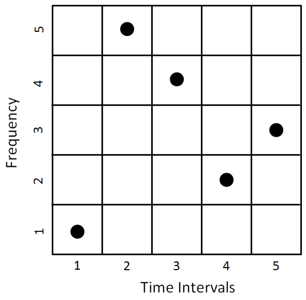
2. Sudoku-Coded Waveforms

An important tool for radar waveform analysis is the ambiguity function, first introduced by Woodward [10]. The ambiguity function characterizes the matched filter output of a radar waveform and is useful for analyzing resolution and ambiguities in delay and Doppler. The radar ambiguity function, $\left|\chi (\tau ,f_d)\right|$, is defined as:

$$\left|\chi (\tau ,f_d)\right|=\left|\frac{1}{2E}{\int }_{-\infty }^{\infty }{S}_1\left(t\right)S_2^{*}(t-\tau )e^{j2\pi f_{d}t}dt\right|,$$

(1)

where $S_1$ is the transmitted signal, $S_2$ is the time-delayed received signal, τ is the time delay, $f_d$ is the Doppler shift and E is the total energy. Often, Equation (1) is termed the auto-ambiguity function if $S_1$ and $S_2$ are the same waveform and likewise the cross-ambiguity function if $S_1$ and $S_2$ are two different waveforms. The cross-ambiguity is of interest in order to gauge the interference from other waveforms.

In the case of a frequency-hopped radar, the signal consists of frequencies chosen from a set $\{f_1,f_2,...f_n\}$ of available frequencies spanning the range $[f_{min},f_{max}]$, where $B=f_{max}-f_{min}$ is the bandwidth and $\Delta f=B/n$ is the frequency spacing, i.e., $\left|f_i-f_j\right|=k\Delta f$ where k is an integer and $1\le i,j\le n$. These frequencies are transmitted at each of a set $\{t_1,t_2,...t_n\}$ of consecutive time intervals, where $T=t_n-t_1$ is the total signal duration and $\Delta t=t_{k+1}-t_k=T/n$ is the time step or the sub-pulse duration, where $2\le k\le n-1$ [11]. Optimum resolutions in both range and Doppler require $\Delta f=1/\Delta t$ [12]. Such a signal can be represented as an $n\times n$ matrix $\mathbf{X}$ shown in Figure 1 where the n vertical rows correspond to the n frequencies and the n horizontal columns correspond to the n time intervals. The matrix entry $x_{pq}$ equals one if and only if frequency $f_p$ is transmitted in time interval $t_q$; otherwise $x_{pq}=0$. Allowing the frequencies to increase or decrease in a linear order over the various time slots would result in a Linear Frequency Modulation (LFM) waveform instead of a more disordered frequency-hopped waveform.

The auto-ambiguity function for the frequency-hopped radar is expressed in terms of coincidence matrices defined as follows. The auto-coincidence matrix of size $(2n-1)\times (2n-1)$ is denoted as χ, and its elements are obtained from the number of the coincidences of the ones of the signal matrix $\mathbf{X}$ between the original array and its translation in both coordinate directions [13]. Each entry of χ, denoted by ${\chi }_{rs}$, represents a shift of r units in the horizontal and s units in the vertical direction. For a shift towards the right, r is positive, while it is negative for a shift towards the left. Similarly, s is positive for a shift upward and negative for a shift downward. The entries of the auto-coincidence matrix χ satisfy the following conditions: ${\chi }_{00}=n$ (this is the autocorrelation), $0\le {\chi }_{rs}<n$ for $(r,s)\ne (0,0)$ when $\left|r\right|\le n-1$ and $\left|s\right|\le n-1$, and ${\chi }_{rs}=0$ if $\left|r\right|>n$ or if $\left|s\right|>n$. For two such signals $\mathbf{X}$ and $\mathbf{Y}$, we define the cross-coincidence matrix ξ of size $(2n-1)\times (2n-1)$ as the number of coincidences of ones between $\mathbf{X}$ and a translated version of $\mathbf{Y}$, shifted to the right or left by r and up or down by s. Ideally, we require ${\xi }_{rs}(\le n)$ for $\left|r\right|\le n-1$ and $\left|s\right|\le n-1$ to be as close to zero as possible in order to ensure orthogonality between $\mathbf{X}$ and $\mathbf{Y}$. Note that ${\xi }_{00}$ represents the cross-correlation between $\mathbf{X}$ and $\mathbf{Y}$.

A specific subset of frequency-coded waveforms are Costas codes, which give what is known as a “thumbtack”-like response for the radar ambiguity function. The longer the codes, the closer the approximation converges to a true “thumbtack” response. Utilizing Sudoku puzzles, we can code the waveforms based on the symbol locations as shown in Figure 2, where the locations of the ones are laid out to demonstrate one possible code. Sudoku has the potential to offer similar performance to that of the Costas codes with the added benefit of many more available codes compared to the finite amount of Costas codes for a given size. One disadvantage is that the distance vectors may not be unique as in the case for Costas-based codes, causing more coincidences to occur.

The ambiguity function $\chi (\tau ,f_d)$ for Sudoku frequency-hopped waveforms is derived from the auto-coincidence matrix by taking into account its finite time duration, as derived in [14] and shown in Equation (2), which is made up of the sum of the auto ${\chi }_{nn}(\tau ,f_d)$ and cross-term ${\chi }_{nm}(\tau ,f_d)$ responses given in Equations (3) and (4), respectively, as follows,

$$\chi (\tau ,f_d)={\chi }_{nn}(\tau ,f_d)+{\chi }_{nm}(\tau ,f_d),$$

(2)

$${\chi }_{nn}(\tau ,f_d)=\frac{1}{N}\sum _{n=0}^{N-1}{e}^{j2\pi f_{d}nT}{e}^{-j2\pi f_n\tau }{e}^{j\pi f_d(T+\tau )}·(1-\frac{\tau }{T})\frac{\sin \left[\pi f_{d}T(1-\frac{\tau }{T})\right]}{\pi f_{d}T(1-\frac{\tau }{T})},$$

(3)

$$\begin{array}{cc}\hfill {\chi }_{nm}(\tau ,f_d)=& \frac{1}{N(N-1)}\sum _{n=0}^{N-1}{e}^{j2\pi f_{d}nT}\sum _{m=0m\ne n}^{N-1}{e}^{-j2\pi f_m[\tau -(n-m)T]}\hfill \\ & ·e^{-j\pi f_{nmd}(NT+\tau )}(1-\frac{\tau }{NT})\frac{\sin \left[\pi f_{nmd}NT(1-\frac{\tau }{NT})\right]}{\pi f_{nmd}NT(1-\frac{\tau }{NT})},\hfill \end{array}$$

(4)

where T is the sub-pulse length, N is the number of chips, $f_m$ is the m-th frequency code, $f_n$ is the n-th frequency code and $f_{nmd}=f_n-f_m-f_d$.

The ambiguity function plot for a Sudoku sequence of length nine corresponding to the ones in Figure 2b is shown in Figure 3a, with the corresponding delay and Doppler cuts in Figure 3b,c. The results are directly comparable to the Costas ambiguity function in which we observe a narrow thumbtack-like peak, which narrows as the number of chips N increases.

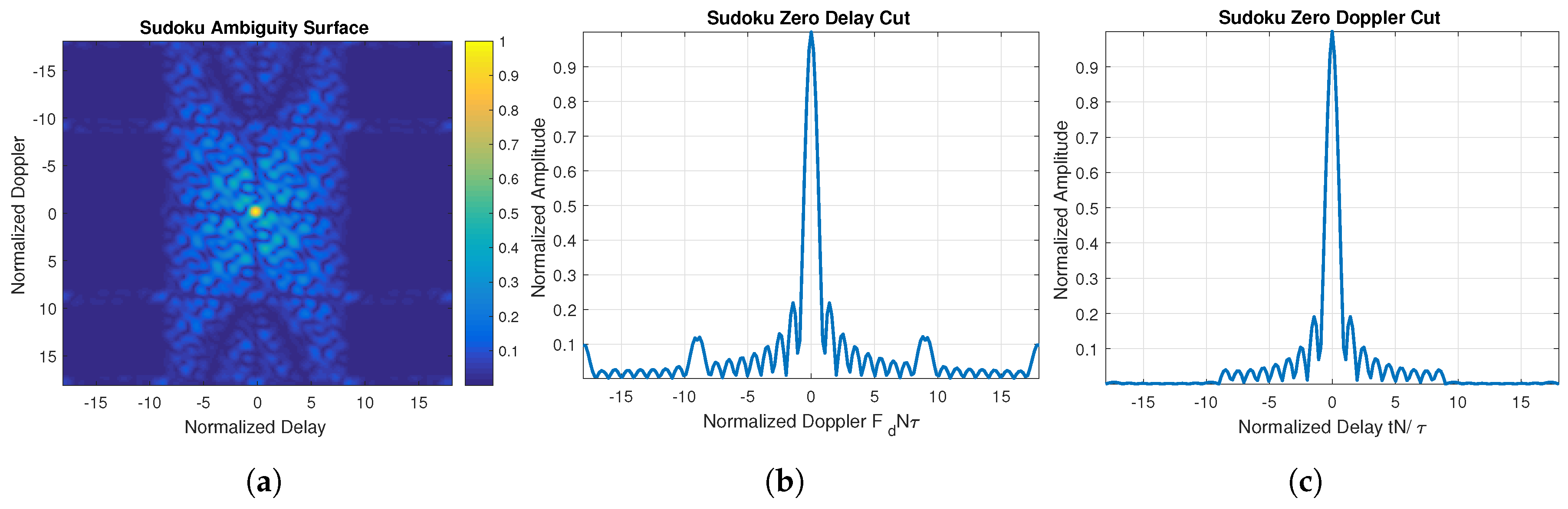
3. Sudoku Ambiguity Function Analysis

Instead of evaluating Equation (2) for side-lobes of multiple sequences, which would be a time-consuming process, we can instead analyze the auto-coincidence and cross-coincidence matrices, which can be performed more efficiently through 2D correlation. The generation of the coincidence matrices was accomplished through the backtracking algorithm for both the Sudoku and the Latin square matrices. The backtracking algorithm recursively solves a given Sudoku or Latin square grid. We start with a blank grid beginning in the upper left corner, continue column wise until we reach the end and then proceed onto the next row. The solver inserts a valid number for a given square from a uniform distribution while checking to make sure it satisfies box, row and column constraints. The algorithm will backtrack to previous squares if no valid numbers solve the current square.

Increasing the Sudoku and Latin square order also increases the number of possible puzzles. While we could easily sort through all $4\times 4$ order matrices, going through $9\times 9$ and even high orders is not feasible. Therefore, we generated a finite number of puzzles and evaluated them for different criteria. Going above a $12\times 12$ Sudoku puzzle was not practical as the computational time for the backtracking algorithm increases significantly for a valid solution; thus, $12\times 12$ was the highest order investigated. The number of puzzles generated was 10,000 for a given size whose auto- and cross-coincidence results are examined in the next section.

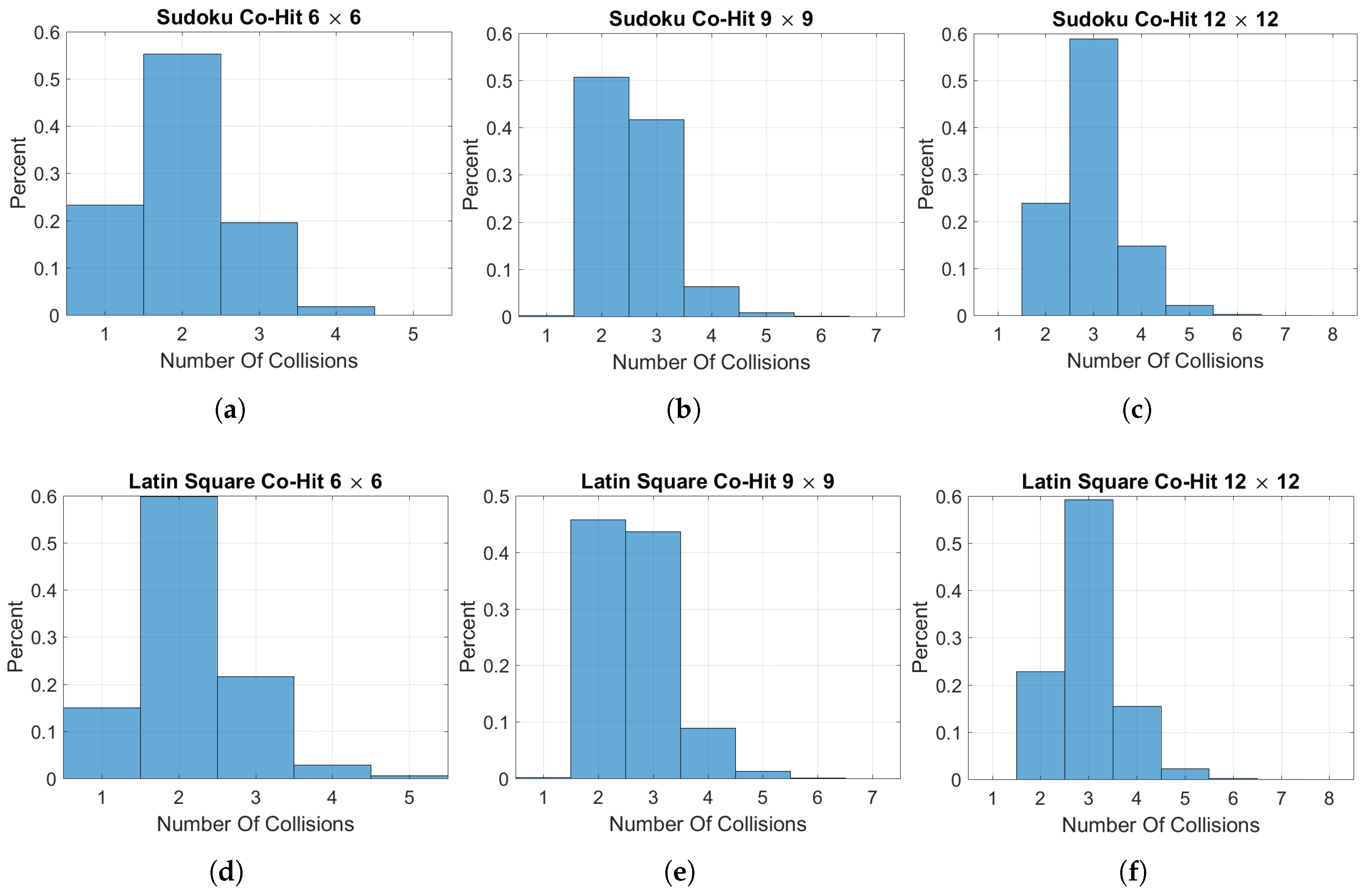
3.1. Sudoku Puzzle Coincidence Analysis

The auto-coincidence matrix or co-hit array is computed by correlating the binary frequency matrix with itself, while the cross-coincidence or cross-hit array is computed by correlating two different frequency codes with each other. By examining the resulting hit array matrices and sorting the resulting collisions in order from greatest to least, we can investigate how well these codes perform. Finding the second highest number of collisions in the co-hit array will give the expected side-lobe performance of that particular code, while the highest number of collisions given in the cross-hit array will give the highest side-lobe coincidence for interference. An example of the coincidence arrays is given in Figure 4.

After the generation of every Sudoku or Latin square, that particular matrix is examined by taking each of the N codes and analyzing their co-hit array performance. Similarly, the cross-hit array performance is analyzed by taking every combination of the N codes and evaluating them among each other.

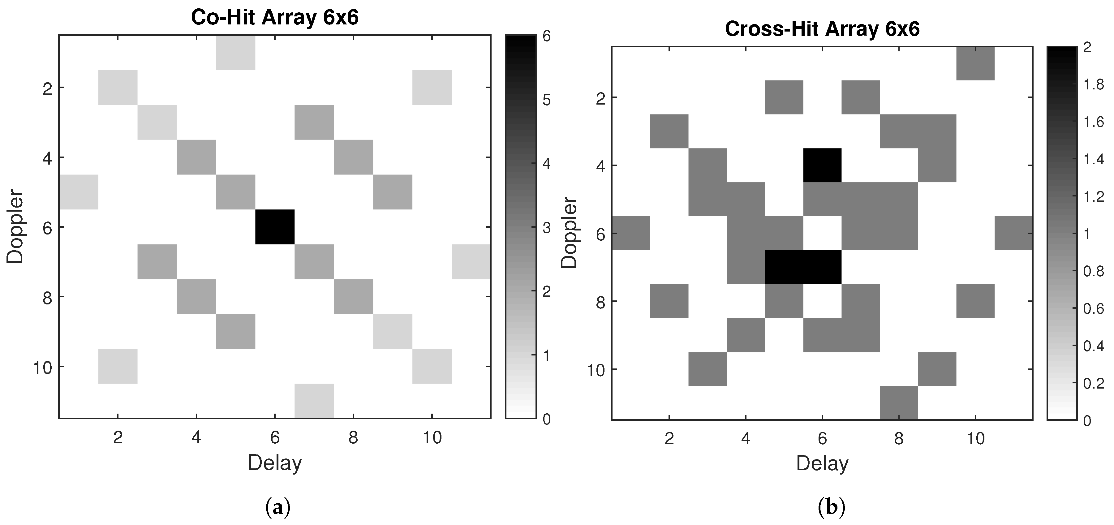
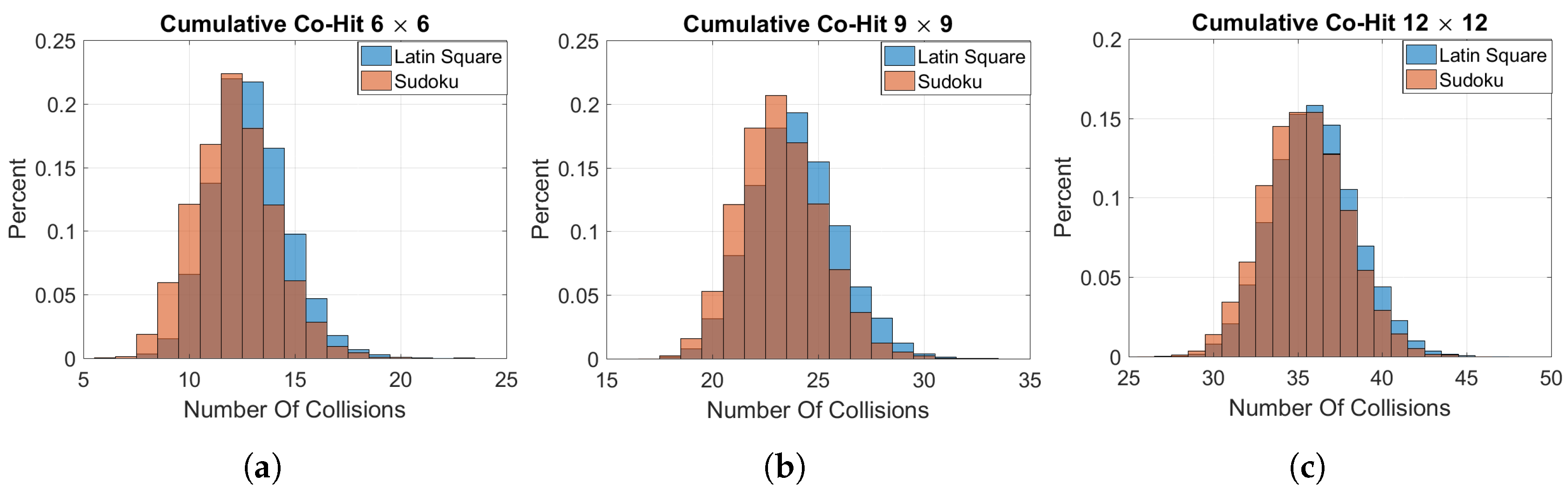
3.1.1. Co-Hit Array Analysis

Histograms displaying the number of auto-coincidences are tabulated for $6\times 6$, $9\times 9$ and $12\times 12$ Sudoku and Latin square matrices and are shown in Figure 5. We observe that the majority of Sudoku puzzles have two or three coincidences with $4\times 4$ containing equal amounts of one and two collisions. As the Sudoku order is increased, we see a shift in the majority of collisions from two to three, with $12\times 12$ having a majority of three. Comparing the Sudoku co-hit arrays with Latin squares, we find that the Sudoku puzzles offer slightly better side-lobe performance with a greater percentage of Sudoku frequency codes offering “one” and “two” numbers of coincidences. The numerical simulations and analysis show that Sudoku frequency codes offer slightly better performance.

Table 1. Percentage of auto-coincidences for Sudoku and Latin squares.

Collisions	1	2	3	4	5	6	7	8
$4\times 4$ Sudoku	50%	50%	0%	0%	0%	0%	0%	0%
$4\times 4$ Latin Square	50%	50%	0%	0%	0%	0%	0%	0%
$6\times 6$ Sudoku	22.21%	55.8%	19.93%	2.04%	0%	0%	0%	0%
$6\times 6$ Latin Square	15.15%	59.5%	21.93%	2.88%	0.50%	0%	0%	0%
$9\times 9$ Sudoku	0.20%	50.24%	42.02%	6.56%	0.88%	0%	0%	0%
$9\times 9$ Latin Square	0.20%	45.54%	44.15%	8.75%	1.15%	0.17%	0.01%	0.0044%
$12\times 12$ Sudoku	0%	24.51%	58.44%	15.16%	1.97%	0.22%	0%	0%
$12\times 12$ Latin Square	0.0025%	22.67%	58.34%	16.24%	2.54%	0.30%	0.033%	0.0042%

shows the percentages of the co-hit array analysis for the different sizes of Sudoku and Latin square matrices. We can see for the Sudoku co-hit array that as the arrays increase in size, the average collision level shifts to the right with the $6\times 6$ averaging two collisions and $12\times 12$ averaging three for the majority. The Latin squares perform similar to the Sudoku matrices with a slightly higher average number of collisions.

Furthermore, we can examine the cumulative coincidences for a given Sudoku or Latin square matrix. The cumulative total is defined as taking a generated matrix and calculating the number of collisions for each of the N codes and summing the total together. Histograms comparing the Sudoku and Latin squares cumulative distributions are shown in Figure 6, where we see that the Sudoku results are slightly shifted to the left, indicating better performance for a particular puzzle order.

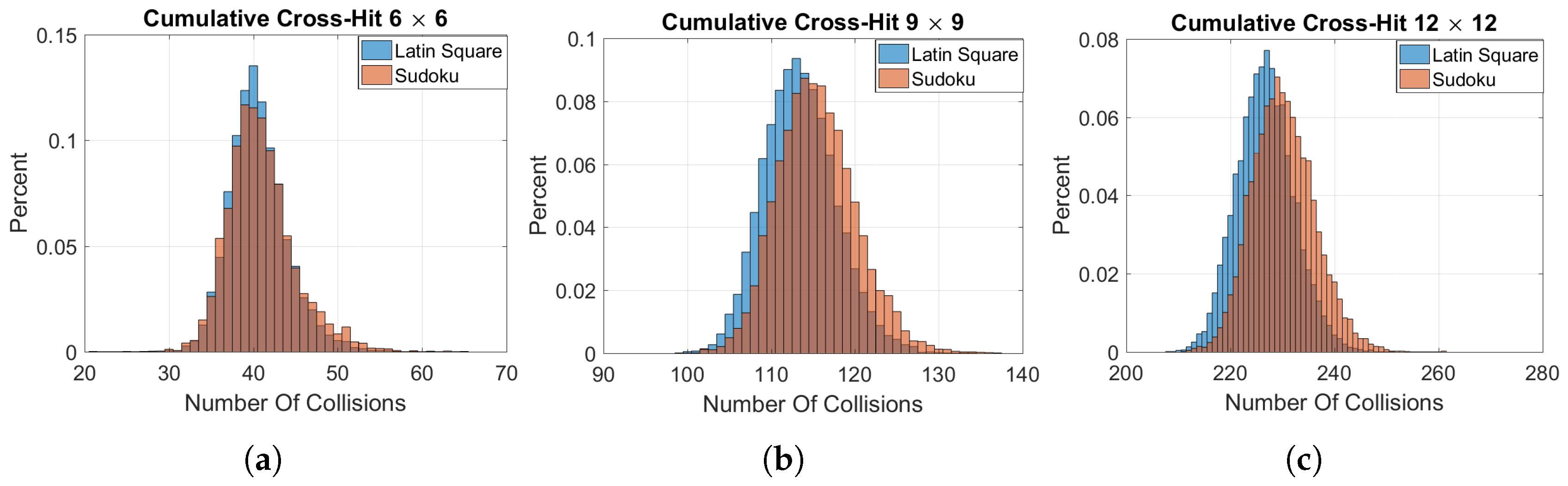
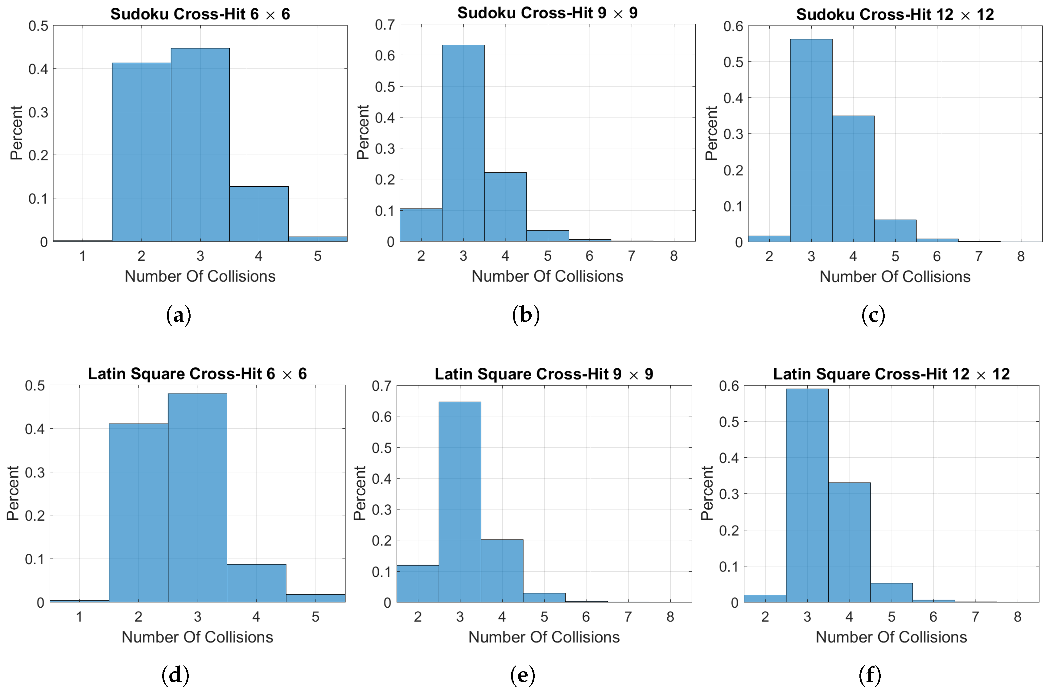
3.1.2. Cross-Hit Array Analysis

The cross-ambiguity function previously mentioned is the matched filter output from two different signals. One reason for exploring cross-ambiguity is to see how interference from other waveforms affects the matched filter output. We compare Latin square permutations to that of the Sudoku solutions by means of the backtracking algorithm. We show results for two different scenarios. First, for a given Sudoku or Latin square matrix, we evaluate the matrix as a whole, i.e., the spread of the cross-hit side-lobes for the N frequency codes. Secondly, we evaluate the cumulative cross-hit arrays for each of the Sudoku and Latin square matrices produced.

Histograms displaying the number of cross-hit coincidences for $6\times 6$, $9\times 9$ and $12\times 12$ Sudoku and Latin square matrices are shown in Figure 7. Viewing these results in graph form rather than tabular form clearly shows the trend of shifting to the right as the order of the Sudoku and Latin square matrices increases.

Table 2. Percentage of cross-coincidences for Sudoku and Latin squares.

Collisions	1	2	3	4	5	6	7
$6\times 6$ Sudoku	0.20%	41.31%	44.6%	12.7%	1.08%	0%	0%
$6\times 6$ Latin Square	0.36%	41.1%	48.6%	8.69%	1.79%	0%	0%
$9\times 9$ Sudoku	0%	10.4%	63.2%	22.2%	3.5%	0.5%	0%
$9\times 9$ Latin Square	0%	11.95%	64.6%	20.2%	2.9%	0.31%	0.02%
$12\times 12$ Sudoku	0%	1.66%	56.28%	34.96%	6.15%	0.8%	0.1%
$12\times 12$ Latin Square	0%	1.97%	59.00%	33.07%	5.24%	0.6%	0.06%

shows the percentages of cross-hit collisions in tabular form. Increasing the Sudoku order causes the majority of cross-hits to increase and shift to the right, and the same can be seen for the Latin square puzzles. The Latin squares show a slightly smaller shift than the Sudoku matrices and therefore perform better for cross-hit collision performance.

The cumulative cross-hit array analysis in Figure 8 shows that indeed, the Latin squares offer better performance in cross-hit collisions, and this effect is more prominent as the order is increased. Comparing these results to the co-hit array results, we can see a trade-off between the co-hit and cross-hit performance of Latin squares and Sudoku-based matrices.

3.2. Costas Sudoku Solutions

Within the Sudoku context, their exists a subset of Sudoku codes that have Costas properties. Starting the search with $4\times 4$ Sudoku matrices, we came across the following solution depicted in Figure 9. Regardless of which number of locations is observed, they are in fact identical with different rotations applied. For example, flipping the twos vertically causes the twos to line up with the fours. Figure 9 shows a $4\times 4$ Sudoku matrix in which every subset of the same number is a Costas sequence, meaning N Costas sequences can form a valid Sudoku puzzle and fit on the same $N\times N$ matrix. Therefore, some Sudoku solutions are in fact Costas arrays. However, not all Costas arrays are Sudoku solutions, as shown in Figure 10, which demonstrates a violation of the Sudoku box constraint.

Another example of a Costas code solution was found when looking at $9\times 9$ Sudoku matrices. The sequence $[9,1,4,5,3,7,6,8,2]$ corresponds to the locations of the ones in the following Sudoku matrix shown in Figure 11. This sequence is a Costas code, but cannot be translated or rotated to fill in the remaining spaces.

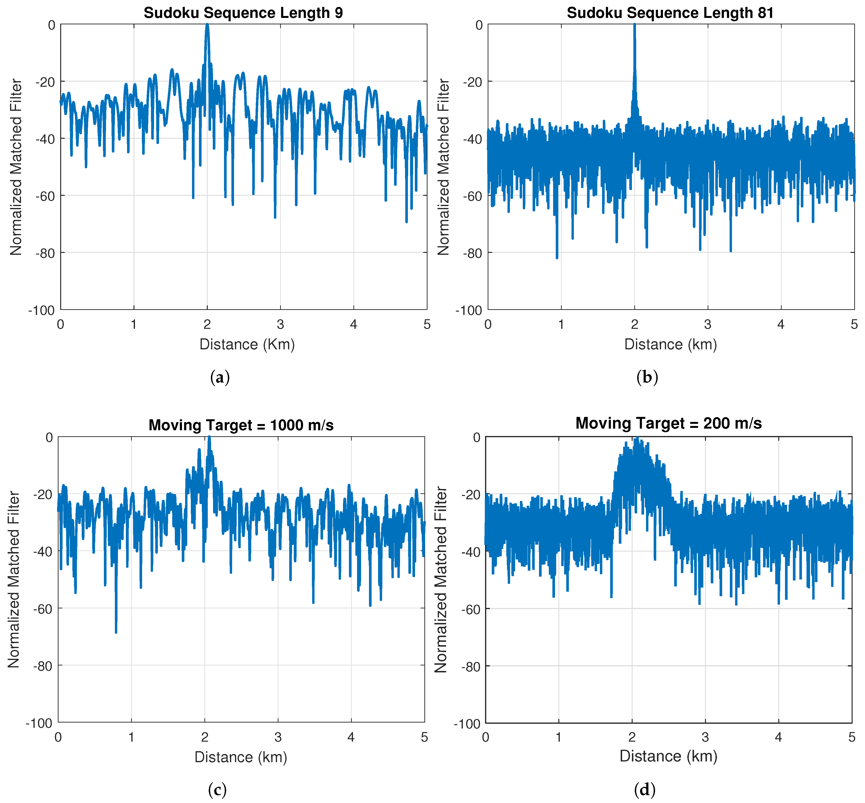
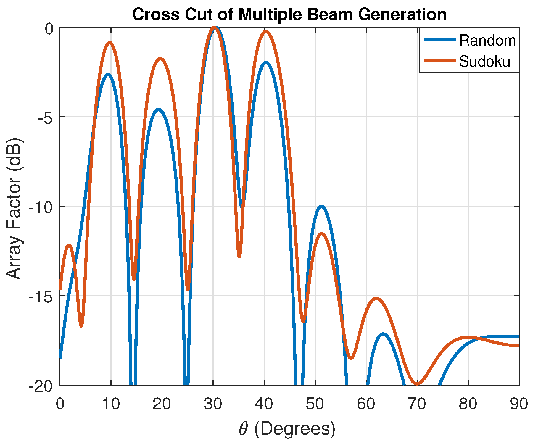
3.3. Sudoku Radar Simulations

Simulated radar target scenarios for single targets were implemented using Sudoku frequency codes. For the frequency-hopped sequence, $x\left(t\right)$, given by [15]:

$$x\left(t\right)=\frac{1}{\sqrt{N{T}_c}}\sum _{n=1}^{M}u(t-n{T}_c),$$

(5)

where N is the number of sub-pulses and $Tc$ is the sub-pulse length. The complex envelope, $u\left(t\right)$, is defined as:

$$u\left(t\right)=\left\{\begin{array}{cc}\exp \left(j2\pi f_{n}t\right),& 0\le t\le T_c\\ 0,& \mathrm{elsewhere}.\end{array}\right.$$

(6)

The frequency of the sub-pulse $F_n$ is given by:

$$F_n=F_0+S_n{\Delta }_f,$$

(7)

where $F_0$ is the carrier frequency, $\Delta f$ is the frequency spacing of the hopped waveform given by $1/Tc$ and S is the frequency-hopped sequence, represented as:

$$S=[a_1,a_2,a_3...a_M].$$

(8)

The parameters of the simulation are given in

Table 3. Radar simulated scenario parameters.

Radar Parameter	Values
Code Lengths	9 and 81
$T_c$	$1\mathsf{\mu }\mathrm{s}$
$F_0$	10 GHz
$\Delta f$	$1/T_c$
Bandwidths	9 MHz and 81 MHz
Target Range	2 km
Radar Cross Section (RCS)	10 ${\mathrm{m}}^2$

where the pulse length and carrier frequency stay constant and the bandwidth is varied based on the code lengths.

Simulation results in Figure 12 pertain to targets located at a range of 2 km: a stationary target and a moving target traveling at speeds of 1000 m/s and 200 m/s with two codes of length nine and 81. We observe in Figure 12a,b for the stationary target case that the longer the hopped sequence, the better the pulse suppression, which is similar to that of Costas frequency-hopped waveforms. When target motion is considered, the results are shown in Figure 12c,d. Similar to the Costas frequency-hopped waveforms, the Sudoku-hopped sequences are not Doppler tolerant in conformance to their ambiguity function results. The longer code length of 81 becomes uncorrelated for much lower velocities compared to the length nine sequence. We know from the ambiguity function plots that the Doppler axis is normalized as given by:

$$f_{d}N{T}_c=\delta f,$$

(9)

where $\delta f$ is the Doppler shift value. Solving for the Doppler shift $f_d$, we can compute the corresponding velocity using:

$$v=\frac{\lambda f_d}{2}.$$

(10)

The resulting velocity depends on the code length, frequency and sub-pulse length; it is easy to observe that as the code length gets longer, the velocity becomes smaller to represent the same Doppler shift. This makes intuitive sense since the longer codes provide a better approximation to the thumbtack-like response.

4. Sudoku Antenna Arrays

We also investigated the application of Sudoku puzzles to antenna array designs, specifically planar arrays. The applications include array interleaving, thinning and random spacing. While no specific design requirements were established when investigating Sudoku for antenna applications, we show that Sudoku antenna designs do indeed offer interesting and useful results for future investigations.

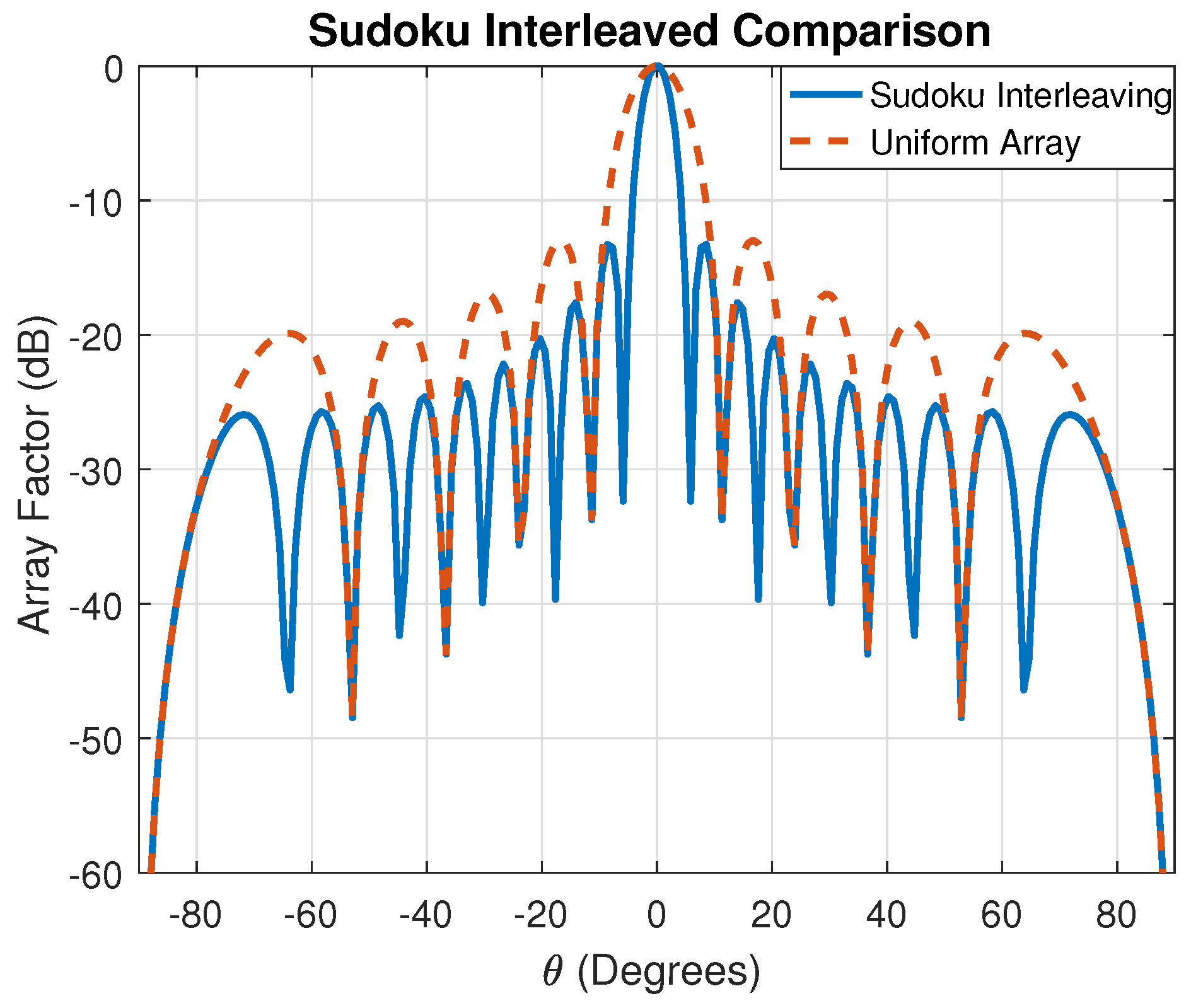
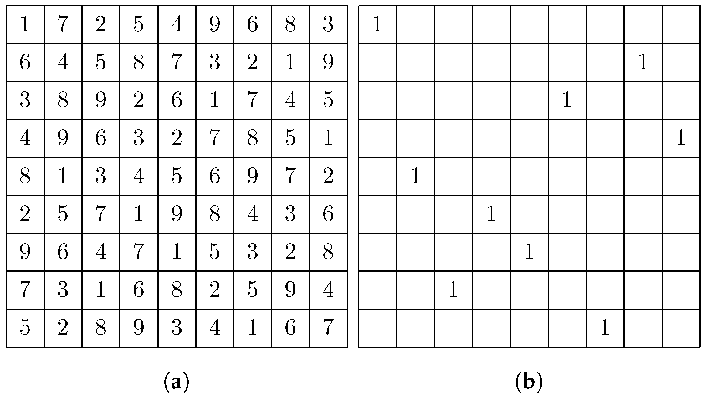
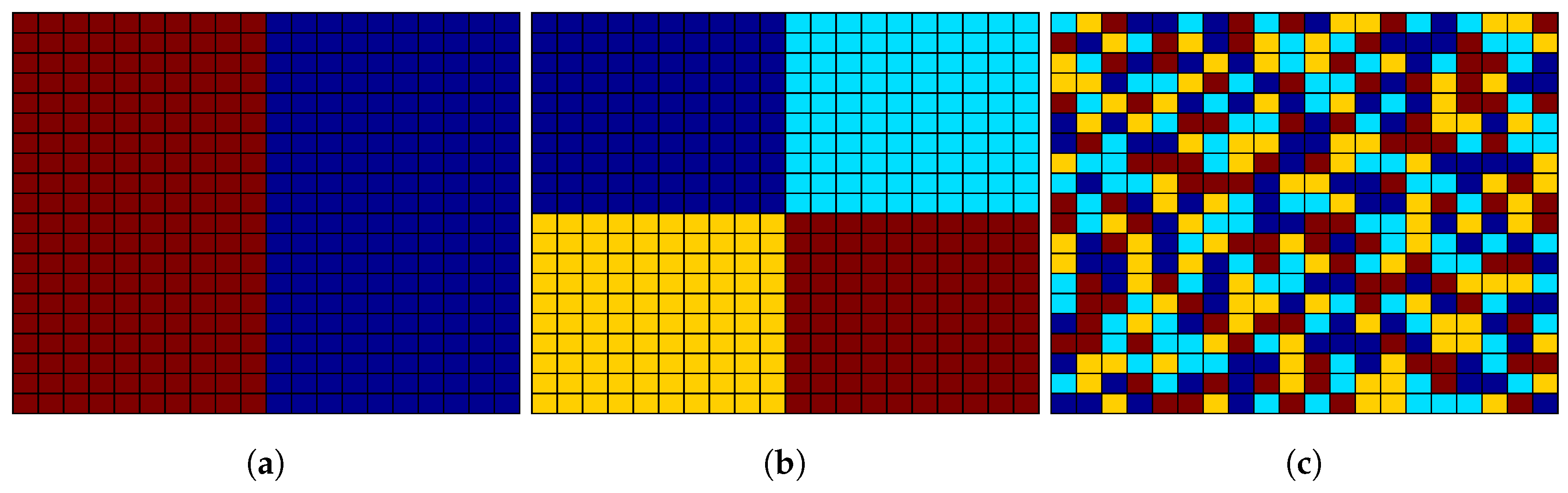
4.1. Sudoku Interleaved Arrays

This section explores two applications of Sudoku puzzles to antenna arrays through interleaving of the elements: (1) main beam steering in multiple directions using a fraction of the array elements; and (2) the generation of simultaneous multiple beams. Array interleaving has been studied previously [16] and is of interest when multiple arrays have to share the same area. Multiple arrangements can be made to have arrays that operate at the same frequency, as shown in Figure 13. Figure 13a shows two arrays positioned side-by-side; Figure 13b shows an arrangement for four arrays; and Figure 13c shows a Sudoku-based interleaving for four arrays. The non-interleaved arrays have better side-lobes, but the interleaved arrays offer narrower beamwidths [16]. The array factor for planar arrays is given by [17]:

$$\begin{array}{c}\hfill AF(\theta ,\varphi )=\sum _{n=1}^N\sum _{m=1}^M{I}_{mn}{\mathrm{e}}^{j{\alpha }_{mn}}{\mathrm{e}}^{j{\xi }_{mn}},\end{array}$$

(11a)

where:

$$\begin{array}{cc}& {\xi }_{mn}=\beta [d_x(m-1)(\sin \theta \cos \varphi -d_y(n-1)\left(\sin \theta \sin \varphi \right)],\hfill \end{array}$$

(11b)

$$\begin{array}{cc}& {\alpha }_{mn}=-\beta [d_x(m-1)(\sin {\theta }_0\cos {\varphi }_0-d_y(n-1)\left(\sin {\theta }_0\sin {\varphi }_0\right)],\hfill \end{array}$$

(11c)

where β is the wave number, $I_{mn}$ is the excitation current for the element at position $(m,n)$, θ and ϕ are the elevation and azimuth angles, respectively, ${\theta }_0$ and ${\varphi }_0$ are the main beam pointing directions, respectively, and $d_x$ and $d_y$ is the element spacing in wavelengths in the x and y directions, respectively. We consider a $20\times 20$ planar array, which consists of 400 elements. The $20\times 20$ array will have four different beams where the Sudoku puzzle is used to separate the elements into four groups based on their numbers as shown in

Table 4. Planar array steering phase groups.

Group Number	1	2	3	4
Numbers	1,2,3,4,5	6,7,8,9,10	11,12,13,14,15	16,17,18,19,20
Scan Angle	$0^{\circ }$	${20}^{\circ }$	${40}^{\circ }$	${60}^{\circ }$

. In other words, 25% of the elements will be used to steer the beam in a desired direction. A comparison of the Sudoku interleaving to that of the quadrant layout in Figure 13b for the XZ plane ($\varphi =0^{\circ }$) is shown in Figure 14, where we can see the narrower beamwidth of the interleaved array.

First, we only consider a single main beam, which is steered to ${40}^{\circ }$ in the θ direction, as well as a single beam steered to ${40}^{\circ }$ in both the θ and ϕ directions. The ideal case in which all elements are turned on is shown in Figure 15.

We next compare the ideal scenarios using two approaches: the first utilizing Sudoku puzzles, while the second being formed by a random permutation of the array elements. The results of the Sudoku and random permutation for a single main beam are shown in Figure 16. The results are normalized to the ideal cases in Figure 15 and, therefore, will have a maximum value lower than 0 dB due to the fraction of elements used. We observe both the Sudoku- and random-based steering result in very similar array factors. The main beam is approximately 12 dB lower than the ideal case and has side-lobes mostly 10 dB below the peak value.

Next, we examine the scenario in which all of the elements are turned on. Therefore, the resulting array factor will have four main beams at the assigned phases given in Table 4 for the case of either the θ direction or θ and ϕ directions. The results for the Sudoku and random multiple beam scenario are shown in Figure 17. The random permutation is normalized to the Sudoku results; therefore, we see that the largest value in the random array is larger than 0 dB. While both scenarios show the main beams, the Sudoku-based approach appears to have a more uniform amplitude across the different beams, while the random case has less uniformity across the beams.

We can examine this more closely in Figure 18, which shows a two-dimensional cross-cut of the two array factors for $\varphi =0^{\circ }$. We can see that indeed the random array does not provide as even an amplitude distribution across the four beams. Obviously, using the random approach, the resulting beam amplitudes could change drastically from each iteration depending on how the element phases get assigned. The Sudoku interleaving approach based on the row, column and box constraints provides a more even spread of the phases across the array, so that a single area of the array is not dominated by a particular phase.

4.2. Array Thinning

Since only a fraction of the elements were used during the investigation of array steering, it was only natural to extend the analysis to array thinning. Large antenna arrays have hundreds of elements where some of the elements can be turned off or removed without drastically altering the resulting array factor. The reduction of antenna elements can save cost, reduce complexity and minimize system weight. Previous research in this area used optimization strategies, such as genetic algorithms, to optimize the removal of elements with respect to a desirable criterion, such as side-lobe level [18]. We investigated the application of a Sudoku rule set so that the resulting array is judiciously thinned. We compared the Sudoku-based approach using an array factor following random element removal. We used the same $20\times 20$ antenna array comprised of 400 elements.

The Sudoku array thinning was compared to random thinning for thinned percentages of 25%, 50% and 75% in Figure 19 with the main beam scanned to ${40}^{\circ }$. The resulting thinned arrays are normalized with respect to the maximum of the ideal array factor in Figure 15a. The results are shown as two-dimensional images with ϕ on the y-axis ranging from $[-180,180]$ degrees and θ on the x-axis ranging from $[0,90]$ degrees.

Generally, the results are quite comparable between the random- and Sudoku-based thinning. The array factor still displays low side-lobe levels of 20 dB when 25% of the elements are removed. As more and more elements are turned off to achieve thinning percentages of 50% and 75%, the side lobes quickly rise, and the array factor is noticeable degraded; however, it appears that the Sudoku thinning shows the side-lobes more clearly distributed around the main beam pointing direction. Comparing the thinned arrays to the ideal case, the main beam amplitude clearly lowers as the elements are removed with 25% of the elements causing approximately a 12-dB loss.

Observing Figure 20a, we show a slice of the thinned Sudoku array factor in the XZ plane ($\varphi =0^{\circ }$). We make a comparison in Figure 20b between an ideal array, represented by the blue line, in which all of the elements are turned on and when the array is thinned to 50%, for both Sudoku- and random-based arrays. The Sudoku- and random-based arrays are normalized to the maximum of the ideal array, resulting in lower amplitude compared to the ideal array factor. We can clearly see that the Sudoku thinning, represented by the red line, has exactly the same array factor as an array that has all of the elements turned on, whereas the random thinning, represented by the yellow line, causes the side-lobes around the main beam to fluctuate and deviate from the ideal array factor.

In order to see why Sudoku thinning keeps the same array side-lobes as an ideal array in the XZ or YZ planes, we examine Figure 21, which shows a $4\times 4$ Sudoku matrix with only the ones present; the rest of the elements are assigned a zero, corresponding to an element that is turned off. Thus, when applying the planar array factor given previously in Equation (11a), the zeros do not contribute to the array factor, while only the ones does. The result of evaluating the summation for the XZ plane ($\varphi =0^{\circ }$; thus $\cos \varphi =1$ and $\sin \varphi =0$) assuming equal element spacing in the x and y directions, ${\theta }_0={\varphi }_0=0$, and the current amplitudes $I_{mn}$ equal to unity, results in,

$$\begin{array}{cc}\hfill AF(\theta ,\varphi )& =1+{\mathrm{e}}^{j\beta d\sin \theta [\cos \varphi +3\sin \varphi ]}+{\mathrm{e}}^{j\beta d\sin \theta [2\cos \varphi +2\sin \varphi ]}+{\mathrm{e}}^{j\beta d\sin \theta [3\cos \varphi +\sin \varphi ]},\hfill \\ & =1+{\mathrm{e}}^{j\beta d\sin \theta }+{\mathrm{e}}^{j2\beta d\sin \theta }+{\mathrm{e}}^{j3\beta d\sin \theta }.\hfill \end{array}$$

(12)

The resulting array factor in Equation (12) clearly represents that of a linear array. A similar result is apparent when evaluating the array factor in the YZ ($\varphi ={90}^{\circ }$) plane. In other words, Sudoku- or Latin square-based thinning removes an element from every row and column resulting in the removal of linear array products.

One might be interested in what advantages, if any, Sudoku-based thinning offers over random thinning or over more robust optimization methods. We believe that Sudoku thinning offers a more uniform thinning of the array since the row, column and subgrid Sudoku constraints cause thinning to not be concentrated in one area, as what could happen in randomly thinning the array. Furthermore, we see good side-lobe behavior within the thinned Sudoku arrays, as well as the cardinal cuts holding the ideal planar array shape.

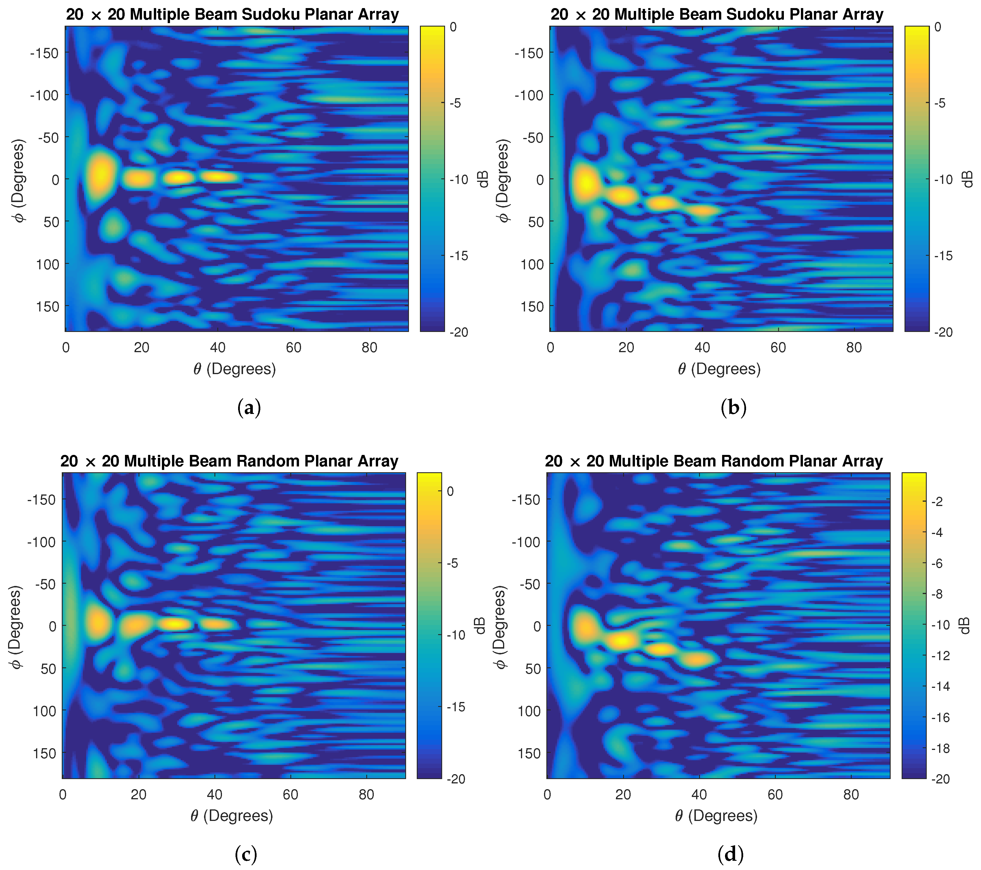
4.3. Random Element Spacing

Owing to the equal element spacing, the periodic arrays are susceptible to grating lobes when the spacing becomes too large for a particular scan angle. Using irregular spacing has the benefit of reducing the appearance of grating lobes while also increasing the bandwidth of the antenna array.

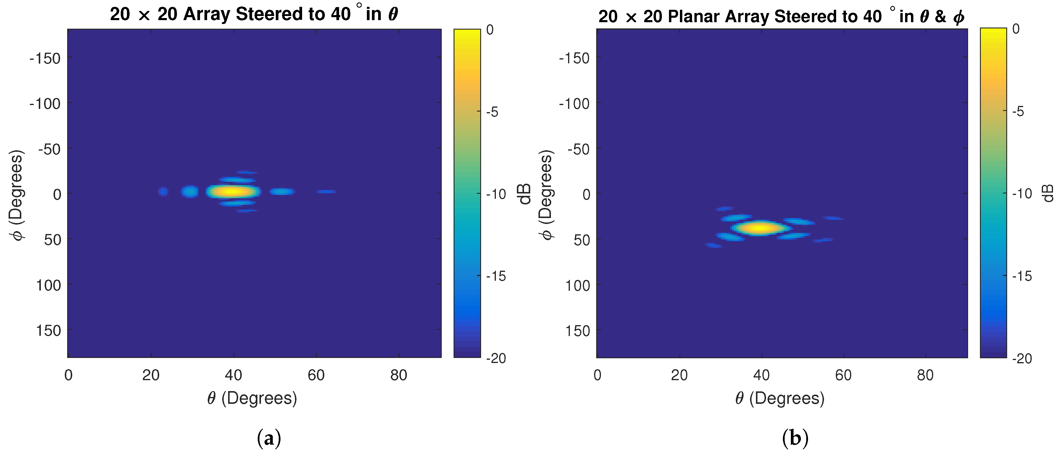
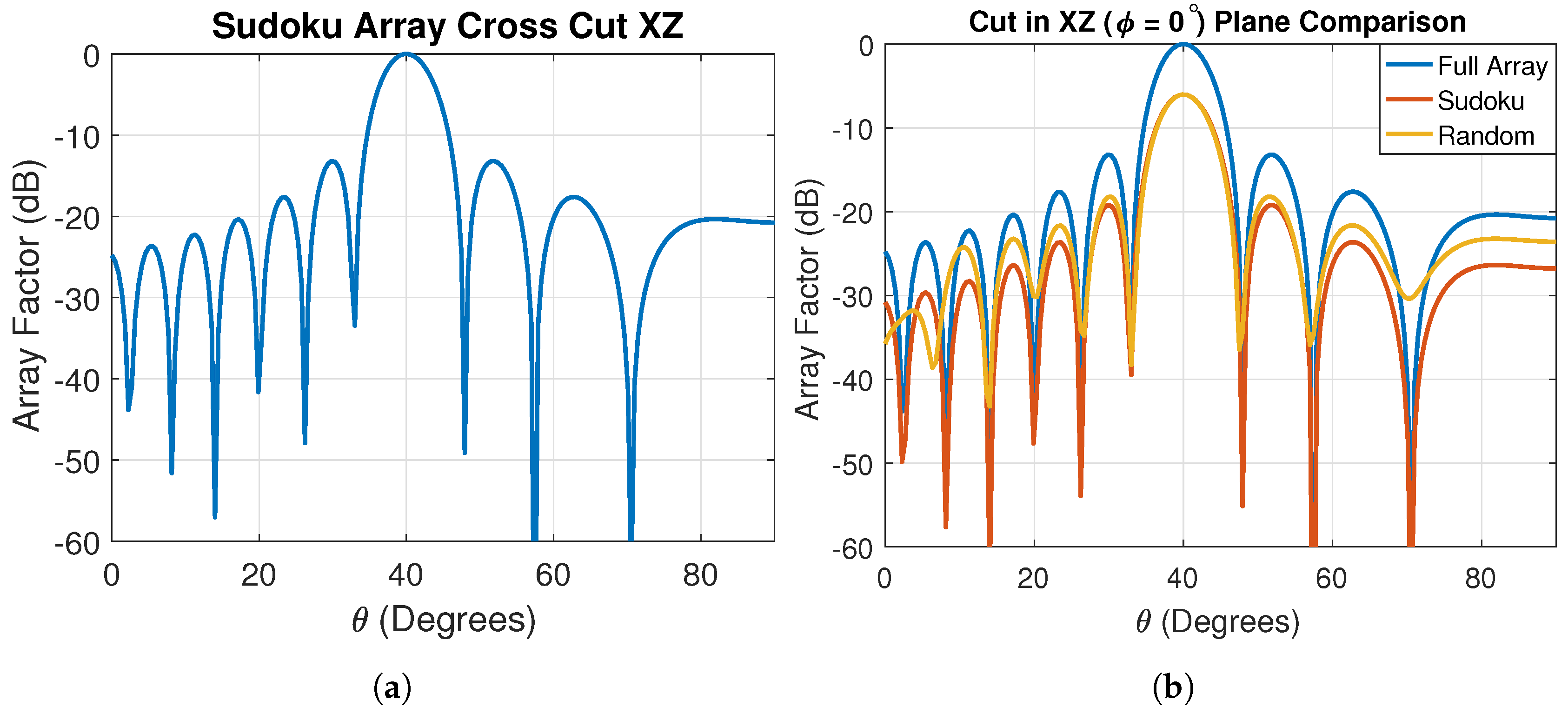
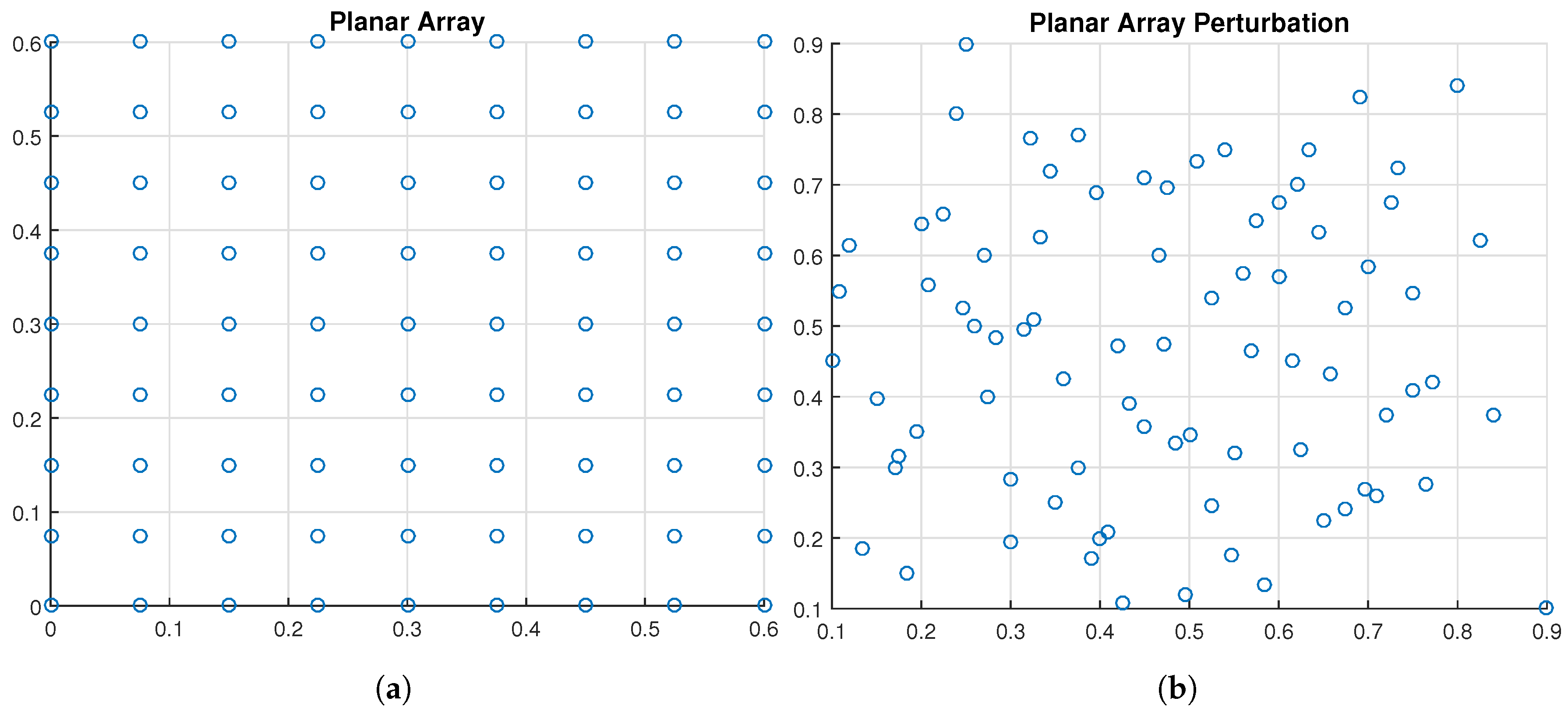
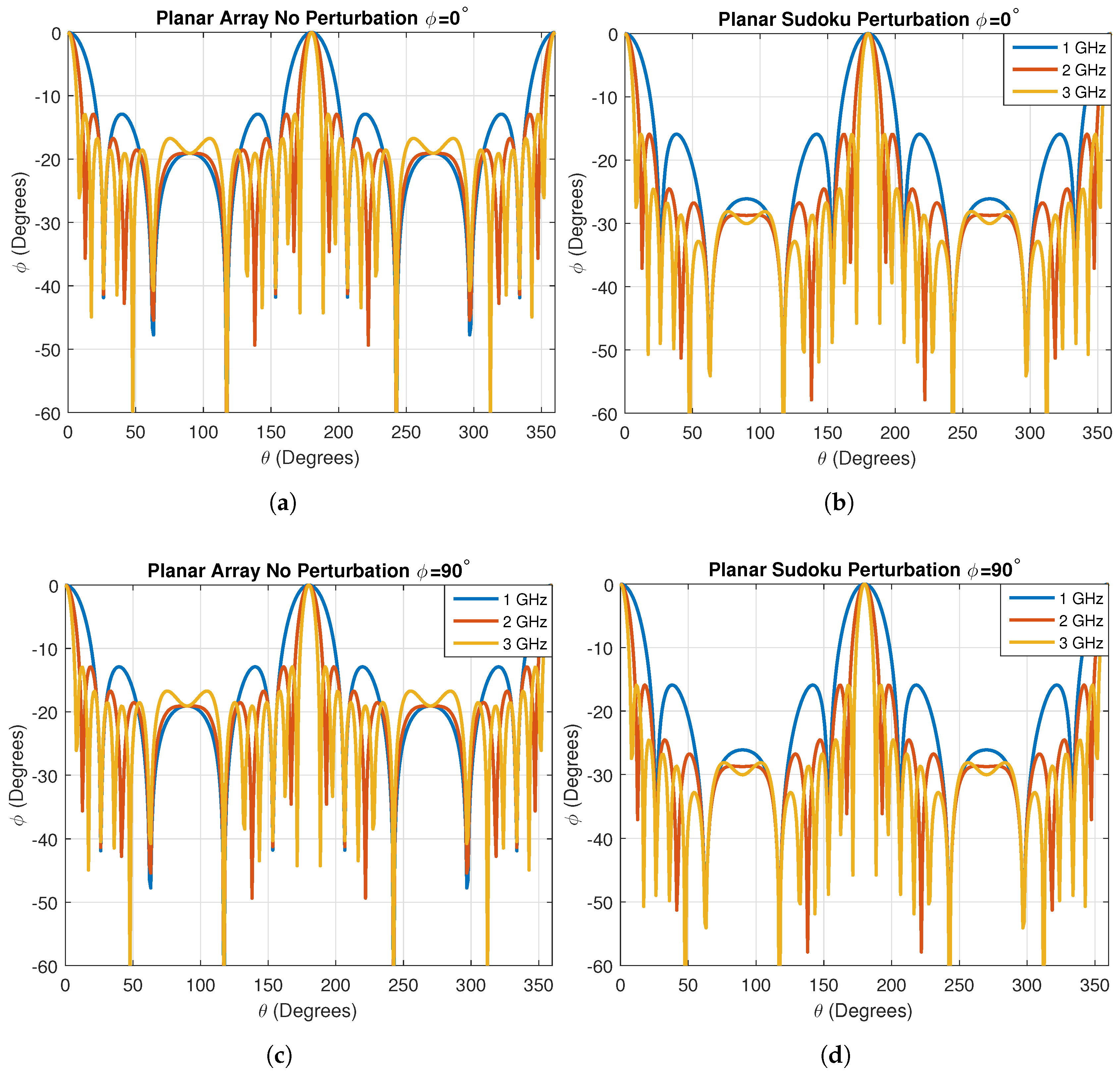
4.4. Perturbed Planar Arrays

We investigate using Sudoku puzzles as perturbations within the planar array of the same size. This is accomplished by modifying the planar array Equation (11a) so that $d_x$ and $d_y$ have an added perturbation δ. The spacing in the x and y directions then become $d_x=d_x+\delta$ and $d_y=d_y+\delta$, respectively. The degree of perturbation comes from the Sudoku puzzle.

First, let us assume we have a $9\times 9$ planar array with ${\lambda }_0=15$ cm corresponding to a frequency of 2 GHz along with equal amplitude excitation of one and uniform spacing of ${\lambda }_0/2$, as shown in Figure 22a.

The generation of two random Sudoku matrices, one for the x-direction and the other for the y-direction, will serve as the perturbations. We would like to add perturbations based on the bandwidth we want the array to operate over; in this case, we consider an operating frequency in the range of 1 to 3 GHz. The bandwidth of 2 GHz was divided evenly among the nine Sudoku numbers, giving nine frequencies spaced 250 MHz apart. The corresponding wavelengths were:

$$\lambda =[0.3,0.24,0.2,0.1714,0.15,0.1333,0.12,0.109,0.1].$$

The number one corresponds to $\lambda =0.3$ cm (f = 1 GHz) and the number nine to $\lambda =0.1$ cm (f = 3 GHz), with the rest of the integers following in decreasing order in wavelength or increasing order in frequency. Utilizing the randomly-generated Sudoku matrices, the numbers were replaced with their respective perturbation values and added to each element during the array factor construction. The output of this procedure is shown in Figure 22b, where we now see that the resulting array has a random-like structure, while also increasing in size by 2${\lambda }_0$.

The size of the array has increased from 0.6λ× 0.6λ to 0.9λ× 0.9λ. We compare the resulting perturbed array to the equally-spaced planar array for the frequencies of 1, 2 and 3 GHz in Figure 23 for $\varphi =0^{\circ }$ and $\varphi ={90}^{\circ }$. We clearly see lower side-lobes in the perturbed array. This suggests that the Sudoku-based perturbations are able to achieve good random arrays, resulting in better side-lobe performance.

5. Conclusions

A detailed investigation into Sudoku-coded waveforms was presented in this paper. We utilized the backtracking algorithm to generate multiple Sudoku puzzles of different sizes to analyze their auto-ambiguity and cross-ambiguity function properties. We compared Sudoku sequences to that of the traditional Latin squares and showed that while Sudoku offers better auto-ambiguity properties, Latin squares offer better cross-ambiguity performance. Furthermore, we showed through our computational search that there exist Costas sequences within Sudoku puzzles and that some Sudoku solutions are in fact all Costas codes. One advantage of the Sudoku sequence is that numerous such sequences are freely available owing to its popularity, making it easy for the radar designer to implement nearly optimal high-resolution waveforms. It has been proven that there are approximately $6.671\times {10}^{21}$ valid Sudoku grids of a size of $9\times 9$ [19], with this number increasing with the order of the Sudoku puzzle. Secondly, the lower number of collisions compared to Latin squares allows for reduced side-lobes.

We also investigated Sudoku puzzles for antenna array applications. While no specific antenna array design requirements were investigated, such as side-lobe level, we show that Sudoku arrays offer unique results. First, we examined Sudoku-based interleaving of multiple arrays used for beam steering, which proved beneficial over randomly assigning the phases to the array by providing a more uniform amplitude across the multiple beams. Secondly, we considered planar array thinning using Sudoku codes as compared to randomly turning off a fraction of the elements. We concluded that Sudoku array thinning leaves the cardinal planes looking like a full antenna array since Sudoku thinning removes linear array products, while randomly removing elements does not. Lastly, we applied Sudoku puzzles to planar arrays to produce a pseudo-random spatial arrangement for reduction in grating lobes across multiple frequencies. Our work demonstrates the usefulness of Sudoku sequences in enhancing the performance of radars and antenna arrays. Future work involves setting specific design goals (e.g., beamwidth, side-lobe level, beam steering angle) and comparing the design of antenna arrays with other popular optimization techniques.

References

1. Keedwell, A.D.; Dénes, J. Latin Squares and their Applications; North Holland: Amsterdam, The Netherlands, 2015. [Google Scholar]
2. Newton, P.K.; DeSalvo, S.A. The Shannon entropy of Sudoku matrices. Proc. R. Soc. A 2010, 466, 1957–1975. [Google Scholar] [CrossRef]
3. Sarkar, J.; Sinha, B.K. Sudoku squares as experimental designs. Resonance 2015, 20, 788–802. [Google Scholar] [CrossRef] [Green Version]
4. Pedersen, R.M.; Vis, T.L. Sets of mutually orthogonal Sudoku Latin squares. Coll. Math. J. 2009, 40, 174–181. [Google Scholar] [CrossRef]
5. Keedwell, A.D. Constructions of complete sets of orthogonal diagonal Sudoku squares. Australas. J. Comb. 2010, 47, 227–238. [Google Scholar]
6. Narayanan, R.M.; Bufler, T.D.; Leshchinskiy, B. Radar ambiguity functions and resolution characteristics of Sudoku-based waveforms. In Proceedings of the IEEE International Radar Conference, Philadelphia, PA, USA, 2–6 May 2016; pp. 17–21.
7. Costas, J.P. A study of a class of detection waveforms having nearly ideal range-Doppler ambiguity properties. Proc. IEEE 1984, 72, 996–1009. [Google Scholar] [CrossRef]
8. Wehner, D.R. High Resolution Radar; Artech House: Norwood, MA, USA, 1987. [Google Scholar]
9. Levanon, N. Radar Principles; John Wiley: New York, NY, USA, 1988. [Google Scholar]
10. Woodward, P.M. Probability and Information Theory with Applications to Radar; Pergamon: New York, NY, USA, 1953. [Google Scholar]
11. Golomb, S.W.; Taylor, H. Constructions and properties of Costas arrays. Proc. IEEE 1984, 72, 1143–1163. [Google Scholar] [CrossRef]
12. Zhang, Y.; Wang, J. Design of frequency-hopping waveforms based on ambiguity function. In Proceedings of the 2nd International Congress on Image and Signal Processing, Tianjin, China, 17–19 October 2009.
13. Chang, W.; Scarbrough, K. Costas arrays with small number of cross-coincidences. IEEE Trans. Aerosp. Electron. Syst. 1989, 25, 109–112. [Google Scholar] [CrossRef]
14. Kang, E.W. Radar System Analysis, Design and Simulation; Artech House: Norwood, MA, USA, 2008. [Google Scholar]
15. Levanon, N.; Mozeson, E. Radar Signals; John Wiley: New York, NY, USA, 2004. [Google Scholar]
16. Haupt, R.L. Antenna Arrays: A Computational Approach; John Wiley: New York, NY, USA, 2010. [Google Scholar]
17. Stutzman, W.L.; Thiele, G.A. Antenna Theory and Design; John Wiley: New York, NY, USA, 2012. [Google Scholar]
18. Haupt, R.L. Thinned arrays using genetic algorithms. IEEE Trans. Antennas Propag. 1994, 42, 993–999. [Google Scholar] [CrossRef]
19. Felgenhauer, B.; Jarvis, F. Enumerating possible Sudoku Grids. Available online: http://www.afjarvis.staff.shef.ac.uk/sudoku/sudoku.pdf (accessed on 1 October 2015).
Figure 1. Frequency-coded waveform matrix. The columns represent the different time intervals, and the rows are the individual frequencies.
Electronics 06 00013 g001
Figure 2. Representative Sudoku puzzle: (a) Sudoku puzzle; (b) same puzzle with only the ones shown.
Electronics 06 00013 g002
Figure 3. Sudoku auto-ambiguity plots: (a) 2D ambiguity surface; (b) zero-delay cut of the Sudoku puzzle; (c) zero-Doppler cut of the Sudoku puzzle.
Electronics 06 00013 g003
Figure 4. Example co-hit and cross-hit arrays: (a) co-hit array for the Sudoku sequence [2,5,4,3,6,1]; (b) cross-hit array for the Sudoku sequences [2,5,4,3,6,1] and [1,3,5,6,4,2].
Electronics 06 00013 g004
Figure 5. Histogram of co-hit array collisions: (a) 6 × 6 Sudoku; (b) 9 × 9 Sudoku; (c) 12 × 12 Sudoku; (d) 6 × 6 Latin square; (e) 9 × 9 Latin square; (f) 12 × 12 Latin square.
Electronics 06 00013 g005
Figure 6. Cumulative co-hit histograms of Sudoku and Latin squares: (a) order 6 × 6 ; (b) order 9 × 9 ; (c) order 12 × 12 .
Electronics 06 00013 g006
Figure 7. Histogram of cross-hit array collisions: (a) 6 × 6 Sudoku; (b) 9 × 9 Sudoku; (c) 12 × 12 Sudoku; (d) 6 × 6 Latin square; (e) 9 × 9 Latin square; (f) 12 × 12 Latin square.
Electronics 06 00013 g007
Figure 8. Cumulative cross-hit histograms of Sudoku and Latin squares: (a) order 6 × 6 ; (b) order 9 × 9 ; (c) order 12 × 12 .
Electronics 06 00013 g008
Figure 9. Sudoku 4 × 4 search result where every number of subset results in a Costas sequence.
Electronics 06 00013 g009
Figure 10. Costas code that is not a valid Sudoku solution.
Electronics 06 00013 g010
Figure 11. A 9 × 9 Sudoku puzzle in which the ones corresponds to a valid Costas code.
Electronics 06 00013 g011
Figure 12. Normalized matched filter output for Sudoku sequences: (a) length nine Sudoku sequence and a single stationary target located 2 km; (b) length 81 Sudoku sequence and a single stationary target located 2 km; (c) length nine Sudoku sequence with a target moving at 1000 m/s; (d) length 81 Sudoku sequence with a target moving at 200 m/s.
Electronics 06 00013 g012
Figure 13. Planar array layout for multiple arrays sharing the same area: (a) side-by-side layout; (b) quadrant layout for four separate arrays; (c) Sudoku-based layout for four arrays.
Electronics 06 00013 g013
Figure 14. Sudoku interleaved array compared to a uniform array quadrant layout.
Electronics 06 00013 g014
Figure 15. A 20 × 20 planar array using all elements: (a) main beam steered to 40 in the θ direction; (b) main beam steered to 40 in both the θ and ϕ directions.
Electronics 06 00013 g015
Figure 16. Single beam steering: (a) Sudoku-based steering for a main beam of 40 in the θ direction; (b) Sudoku-based steering for a main beam of 40 in both the θ and ϕ directions; (c) random-based steering for a main beam of 40 in the θ direction; (d) random-based steering for a main beam of 40 in both the θ and ϕ directions.
Electronics 06 00013 g016
Figure 17. Multiple beam steering: (a) Sudoku-based steering for beams of 10 , 20 , 30 , 40 in the θ direction; (b) Sudoku-based steering for main beams of 10 , 20 , 30 , 40 in both the θ and ϕ directions; (c) random-based steering for main beams of 10 , 20 , 30 , 40 in the θ directions; (d) random-based steering for main beams of 10 , 20 , 30 , 40 in both the θ and ϕ directions.
Electronics 06 00013 g017
Figure 18. Cross-cut for ϕ = 0 for the Sudoku- and random-based arrays.
Electronics 06 00013 g018
Figure 19. Thinned 20 × 20 planar array using random- and Sudoku-based thinning: (a) random thinning of 25%; (b) random thinning of 50%; (c) random thinning of 75%; (d) Sudoku thinning of 25%; (e) Sudoku thinning of 50%; (f) Sudoku thinning of 75%.
Electronics 06 00013 g019
Figure 20. Cross-cut of the scanned 20 × 20 planar array: (a) thinned Sudoku array cross-cut in the XZ plane; (b) comparison of the Sudoku- and randomly-thinned array factor to that of an array with all of the elements turned on.
Electronics 06 00013 g020
Figure 21. A 4 × 4 Sudoku array with only the ones present to study the effects of turning off elements with row, column and subgrid constraints.
Electronics 06 00013 g021
Figure 22. Array topology: (a) planar array with λ / 2 spacing corresponding to 2 GHz; (b) planar array with Sudoku-based perturbations.
Electronics 06 00013 g022
Figure 23. Planar array with spacing equal to the center frequency of 2 GHz: (a) no perturbation for ϕ = 0 ; (b) Sudoku perturbation for ϕ = 0 ; (c) no perturbation for ϕ = 90 ; (d) Sudoku perturbation for ϕ = 90 .
Electronics 06 00013 g023