Compressed Sensing ISAR Reconstruction Considering Highly Maneuvering Motion

Abstract

In this report, we propose compressed sensing inverse synthetic aperture radar (ISAR) imaging in the presence of highly maneuvering motion using a modified orthogonal matching pursuit (OMP) reconstruction algorithm. Unlike existing methods where motion is limited to first- or second-order phase terms, we take into account realistic motion of a maneuvering target that can involve a third-order phase term corresponding to the rate of rotational acceleration. In addition, unlike existing fixed dictionary-based methods, which require designing a large dictionary that needs to take into account all of the possible motion parameters, we propose a modified OMP reconstruction method that requires a dictionary only based on the first-order phase term and estimates the second- and third-order phase terms using an optimization algorithm. Simulation examples and comparison with existing methods show the viability of our approach for imaging moving targets consisting of higher order motion.

1. Introduction

Compressed sensing (CS) has demonstrated that a signal sparse in a certain dictionary can be undersampled to a certain extent and recovered without any aliasing artifacts. The undersampling would mean that a signal can be converted into a digital form using a lower number of samples compared to those required by the Nyquist sampling theorem. This undersampling can lead to benefits, such as reduced data acquisition time, lower data sampling, resulting in smaller data size, helping in compressing the original signal, etc. The undersampled data are processed by solving an optimization problem that consists of minimization of the $l_1$ and $l_2$ norms resulting in a high-resolution reconstruction.

The theory of CS has been developed in many works, including [1,2,3,4]. The solutions of the optimization problem involved in CS can be obtained by several techniques, such as orthogonal matching pursuit (OMP) [5], Bayesian CS [6], Bayesian matching pursuit [7,8], modified quasi-Newton method [9], etc. Similarly, applications of CS have been demonstrated in different works, such as single-pixel remote sensing [10], tomographic SAR [11] , through-the-wall imaging for stationary and moving targets [12] , radar imaging [13,14,15], passive radar imaging [16], sparse microwave imaging of perfect electric conducting targets [17], etc.

Compressed sensing has also been applied to inverse synthetic aperture radar (ISAR) imaging mainly to image in the presence of rotational motion. Inaccurate knowledge of this motion can cause blurring in the processed image. Initially, this application was concerned with generating high-resolution images of ISAR undersampled data with limited or uniform rotational motion. The limited motion would mean that the received data would consist of constant-frequency exponential terms due to the absence of any acceleration. The data would require only a Fourier transform (FT) to recover the position and reflectivity of the moving points. Undersampling of the data would normally mean that an FT would result in artifacts, resulting in blurred images.

Compressed sensing was initially applied to the case of limited motion mentioned above, where it was used to replace the FT. The work in [18] examined this situation and showed that aliasing effects due to undersampling could be compensated and a high-resolution 2D image could be obtained by using a fixed dictionary based on limited rotational motion that causes a first-order phase term. Other techniques include [19,20,21] that mainly deal with objects undergoing uniform rotational motion resulting in a second-order phase term that is directly dependent on the first-order phase term. The authors in [19,20,21] used a parametric dictionary for reconstruction.

The condition of limited motion in a realistic scenario would require an object to be imaged for a short time, to ensure that the object moved almost uniformly during the imaging. However, to meet this requirement for a maneuvering motion, a very short observation time is needed, resulting in the recovery of a low number of scatterers. This would lead to an image that becomes less discernible, as shown in [18]. Hence, other CS-based techniques were proposed that could cater to a higher-order or non-uniform motion involving acceleration.

To deal with non-uniform rotation, a new dictionary was presented in [22] that could deal with both first-order rotational velocity and second-order rotational acceleration phase terms. An analysis was also carried out to quantify the effects of spacing of different parameters in the dictionary on the imaging performance, because any mismatch of dictionary elements from the compressively-sensed data can limit the imaging performance of CS, as shown in [23,24]. The work in [25] considered uniform and non-uniform rotational motion in the presence of unavailable or corrupted data and demonstrated the application of quadratic time-frequency-based representation for CS imaging when rotational acceleration was present in the data. It was shown in [26] that in case of high maneuverability of an observed target, the received data are multi-component phase signals. In this scenario, an approach limiting motion till a second-order phase term representing rotation rate and rotational acceleration has its limitations, as shown in [22].

A further review of some existing work on CS ISAR imaging is as follows: The work in [27] proposed sparse imaging to compensate for range migration in the presence of uniform rotational motion making use of Bayesian sparse representation. The proposed imaging was divided into two steps: a coarse imaging carried out based on the minimum entropy criterion and a residual phase error correction performed using a 2D Fourier dictionary. The work in [28] proposed a 2D CS-based reconstruction for a target containing translational motion and a small-angle rotation with limited motion, by decoupling translational and rotational motions and carrying out CS imaging in range and azimuth directions separately.

The work in [29] proposed an autofocus-based technique to compensate for phase errors arising due to imperfect translational motion compensation based on sparse Bayesian learning. The target was assumed to be rotating uniformly, and these phase errors due to imperfect translational motion compensation could affect the focusing in azimuth direction. The work in [30] also proposed an autofocus-based technique to compensate for translational motion assuming uniform rotation motion. This technique was based on estimating translational motion as a polynomial and estimating the coefficients of the polynomial using the particle swarm optimization algorithm.

The work in [31] showed that the CS formulation directly in 2D instead of the traditional 1D stacking approach could be used for generating high-resolution images and could deal with compressed data that have a few missing samples, or gapped data that can have a large number of missing samples. The authors assumed small rotation and a dictionary based on Fourier matrices. The work in [32] applied Bayesian CS and used a parametric dictionary for CS ISAR imaging in the presence of uniform rotation. The work in [33] used a 2D CS ISAR imaging considering uniform rotational motion and used dictionaries based on non-uniform Fourier transform for both range and azimuth directions.

The work in [34] proposed CS ISAR image representation based on a sparsity prior and non-local total variation that reconstructs strong scatterers in an observed object and maintains the overall shape of the object, respectively. The authors assumed a uniform rotation rate and a Fourier basis matrix. The work in [35] used a parametric sparse representation to compensate for platform motion errors in SAR that improves the imaging quality compared to other autofocus methods. The imaging consisted of estimating the reflectivities of the scatterers, followed by calculating azimuth velocity errors and range acceleration errors represented by a linear chirp rate for these errors, which can be seen as equivalent to estimating the rotational acceleration for ISAR.

Compared to the above-mentioned references that mainly deal with CS ISAR imaging in the presence of rotational motion limited to first- or second-order phase terms, the novel contributions of our report are: (1) We deal with imaging from compressively-sensed data in the presence of motion in the case of highly maneuvering targets. This rotational motion consists of a first-order phase term due to rotation rate or velocity, a second-order phase term due to rotational acceleration and a third-order phase term due to the rate of rotational acceleration, which is ignored in the previously-mentioned word. Ignoring the rate of rotational acceleration would lead to motion artifacts in the reconstructed imagery; (2) We analyze the performance of a dictionary-based reconstruction in order to deal with highly maneuvering motion and show that due to the dependence of reconstruction error on both rotational acceleration and the rate of rotational acceleration, a very small spacing should be maintained between different parameters of the dictionary. This would lead to a dictionary of a huge size, resulting in very high storage and computation requirements; (3) We then propose a dictionary-less CS ISAR reconstruction by modifying parts of the OMP algorithm that consists of using an optimization algorithm to find the position, rotational acceleration and the rate of rotational acceleration. We further show that to reduce reconstruction errors and reduce the search space for the optimization algorithm, a hybrid dictionary-based and dictionary-less CS ISAR approach can be used where the grid corresponding to position is supposed to be known or over-sampled, and the rotational acceleration and rotational acceleration rate are estimated using a parametric dictionary.

The present report is organized as follows: Section 2 presents the observation model used in the report, as well as a basic CS reconstruction perspective for this problem. Section 3 details the proposed methodology for reconstruction and analysis for ISAR imaging in the presence of highly maneuvering motion. Section 4 presents imaging and numerical results using the proposed approach, followed by conclusions in Section 5.

2. Compressed Sensing Inverse Synthetic Aperture Radar

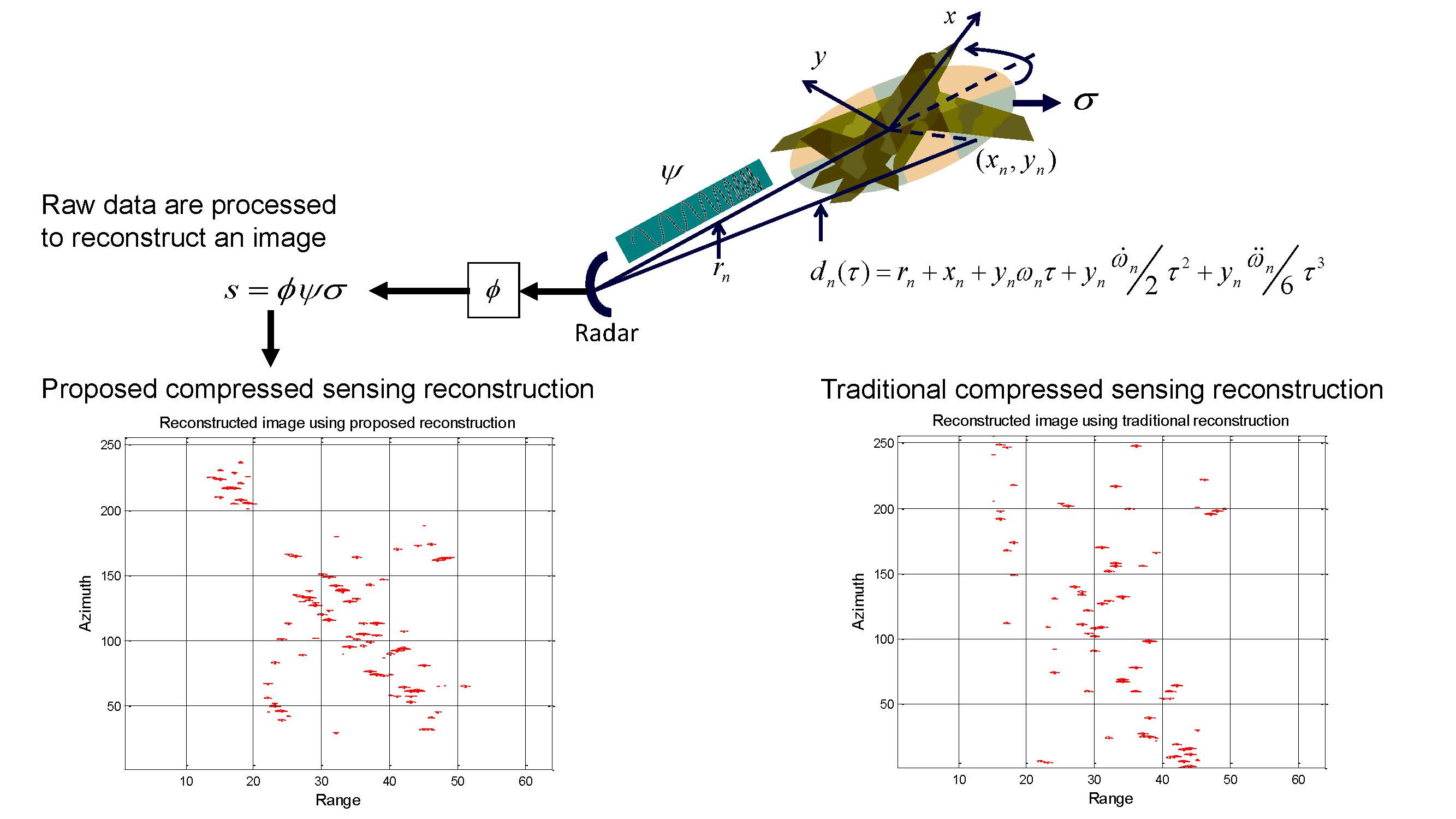
2.1. Observation Model

In this report, x denotes a scalar; $\mathit{x}$ denotes a vector; and $\mathit{X}$ denotes a matrix. We use ${\mathit{x}}^{\prime }$ to denote the transpose of $\mathit{x}$. The same notation is used for Greek characters. We consider range-compressed and range-aligned ISAR data, where any range-walk due to translational motion has been eliminated using traditional methods. Therefore, the data are aligned along the azimuth direction for each range bin. Such data, corresponding to one range bin and a point n, can be written as:

$$s_n(\tau )={\sigma }_n{p}_n(\tau )$$

(1)

where τ is the along-track time sampled at a frequency $f_{\tau }$, i.e., $\tau =0,{\displaystyle \frac{1}{f_{\tau }}},{\displaystyle \frac{2}{f_{\tau }}},....,{\displaystyle \frac{N_{\tau }-1}{f_{\tau }}}$ with $N_{\tau }$ being the total number of along-track time samples. The reflectivity of the point n is given by ${\sigma }_n$, and $p_n(\tau )$ describes the range-aligned signal based on the rotational motion of the target as follows:

$$p_n(\tau )=\mathrm{rect}\left(\frac{\tau }{T_{\tau }}\right)exp\left(-j{k}_c{d}_n(\tau )\right)$$

(2)

where $\mathrm{rect}\left({\displaystyle \frac{\tau }{T_{\tau }}}\right)$ is a limit on the pulse size according to pulse-width $T_{\tau }$ arising from the total target observation time in azimuth direction and $k_c$ is the wavenumber defined as $k_c=\frac{4\pi f_c}{c}$.

The azimuth time-varying radar-target distance $d_n(\tau )$ for the n-th point rotating with an angle $\Delta {\theta }_n(\tau )$ is approximated as [36]:

$$d_n(\tau )=r_n+x_n+y_n\Delta {\theta }_n(\tau )$$

(3)

The slant-range distance to the rotation center of the observed moving point is represented by $r_n$; $x_n$ and $y_n$ denote the range and azimuth distance of the point from the rotation center, respectively.

Using the value of $d_n(\tau )$ given by Equation (3) in Equation (2) and retaining only the azimuth time-dependent part, we get:

$$p_n(\tau )=\mathrm{rect}\left(\frac{\tau }{T_{\tau }}\right)exp\left(-j{k}_c{y}_n\Delta {\theta }_n(\tau )\right)$$

(4)

The total range-compressed and aligned raw data for a total number of N moving points in a single range bin can then be written as the sum of received data from each point as follows [37]:

$$s_0(\tau )=\sum _{n=1}^N{s}_n(\tau )=\sum _{n=1}^N{\sigma }_n{p}_n(\tau )$$

(5)

In existing literature on CS ISAR, $\Delta {\theta }_n(\tau )$ is either approximated as consisting of a first-order term:

$$\Delta {\theta }_n(\tau )\approx {\omega }_n\tau$$

(6)

or up to a second-order term as follows:

$$\Delta {\theta }_n(\tau )\approx {\omega }_n\tau +\frac{1}{2}{\dot{\omega }}_n{\tau }^2$$

(7)

where ${\omega }_n$ is rotational velocity and ${\dot{\omega }}_n$ is rotational acceleration. Let ${\alpha }_n=k_c{y}_n{\omega }_n$ be defined as the rotation rate phase term. It can be further written as ${\alpha }_n=2\pi d_n\Delta f$, where $d_n$ gives the azimuth frequency/Doppler pixel position of the scatterer corresponding to the phase term ${\alpha }_n$, and $\Delta f=\frac{f_{\tau }}{N_{\tau }}$ is the frequency resolution. Our goal is to estimate $d_n$ to form a processed image showing the position of the scatterer in the azimuth frequency/Doppler location. In addition, we define ${\beta }_n=\frac{k_c}{2}{y}_n{\dot{\omega }}_n$ as the rotational acceleration phase term. The resulting expression for $p_n(\tau )$ can be re-written as:

$$p_n(\tau ,{\alpha }_n,{\beta }_n)=\mathrm{rect}\left(\frac{\tau }{T_{\tau }}\right)exp\left(-j{\alpha }_n\tau -j{\beta }_n{\tau }^2\right)$$

(8)

Using these notations, we can create a dictionary that represents range-compressed and aligned ISAR raw data for $N_{\alpha }$ and $N_{\beta }$ possible rotational velocity and rotational acceleration, i.e., ${\alpha }_1,{\alpha }_2,....,{\alpha }_{N_{\alpha }}$ and ${\beta }_1,{\beta }_2,....,{\beta }_{N_{\beta }}$, respectively. This dictionary is defined as:

$$\mathsf{\Psi }=[{\mathit{\psi }}_{{\alpha }_1,{\beta }_1},{\mathit{\psi }}_{{\alpha }_2,{\beta }_1},....,{\mathit{\psi }}_{{\alpha }_{N_{\alpha }},{\beta }_1},....,{\mathit{\psi }}_{{\alpha }_1,{\beta }_{N_{\beta }}},{\mathit{\psi }}_{{\alpha }_2,{\beta }_{N_{\beta }}},....,{\mathit{\psi }}_{{\alpha }_{N_{\alpha }},{\beta }_{N_{\beta }}}]$$

(9)

with dimensions $N_{\tau }\times N_{\alpha ,\beta }$, where $N_{\alpha ,\beta }=N_{\alpha }\times N_{\beta }$.

Each entry of the dictionary is further given as:

$${\mathit{\psi }}_{{\alpha }_n,{\beta }_n}={\left[p_n(0,{\alpha }_n,{\beta }_n),p_n\left(\frac{1}{f_{\tau }},{\alpha }_n,{\beta }_n\right),\dots ,p_n\left(\frac{N_{\tau }-1}{f_{\tau }},{\alpha }_n,{\beta }_n\right)\right]}^{\prime }$$

(10)

We further define the reflectivity to be consisting of an $N_{\alpha ,\beta }\times 1$ column vector σ, where an entry $\sigma ({\alpha }_n,{\beta }_n)$ corresponds to the reflectivity for values ${\alpha }_n$ and ${\beta }_n$. The reflectivity is given as follows:

$$\mathit{\sigma }={\left[\sigma ({\alpha }_1,{\beta }_1),\dots ,\sigma ({\alpha }_{N_{\alpha }},{\beta }_1),\sigma ({\alpha }_1,{\beta }_2),\dots ,\sigma ({\alpha }_{N_{\alpha }},{\beta }_2),\dots ,\sigma ({\alpha }_1,{\beta }_{N_{\beta }}),\dots ,\sigma ({\alpha }_{N_{\alpha }},{\beta }_{N_{\beta }})\right]}^{\prime }$$

(11)

In order to represent a particular scenario of CS imaging, where the received data may have been downsampled by a factor D, a sampling matrix Φ of size $\frac{N_{\tau }}{D}\times N_{\tau }$ is defined as follows:

$$\begin{array}{c}\hfill \mathsf{\Phi }=\left[\begin{array}{cccccccc}1& 0& 0& 0& .& .& .& 0\\ 0& 0& 1& 0& .& .& .& 0\\ .& .& .& .& .& .& .& .\\ .& .& .& .& .& .& .& .\\ .& .& .& .& .& .& .& .\\ 0& 0& 0& 0& .& .& .& 1\end{array}\right]\end{array}$$

(12)

A position of 1 at the d-th column in a particular row of Φ would mean that we select only the d-th row from Ψ. We further define $M=\frac{N_{\tau }}{D}$ for the ease of notation.

The received undersampled SAR raw data $\mathit{s}$ for each range bin can be subsequently written as:

$$\mathit{s}=\mathsf{\Phi }\mathsf{\Psi }\mathsf{\sigma }+\mathit{\epsilon }$$

(13)

The individual elements in Ψ take into account the rotational rate and rotational acceleration.

2.2. Reconstruction

The received data are of size $M\times 1$, where $M<N_{\tau }$, meaning that there are more unknowns than given equations. As recovering σ from $\mathit{s}$ in Equation (13) is an under-determined problem, it can be solved under the following conditions:

• The reflectivity vector σ is sparse, which means that many of its entries are zeros or of very small magnitude. This is a valid assumption in CS ISAR imaging as there are a few strong reflecting points in an object for each range bin.
• For a sparsity level K, the number of linearly independent measurements should be at least [38]:

  $$M=2K$$

  (14)
  This condition ensures that we can recover an original signal with sparsity K without any ambiguity. In the literature, various expressions for the minimum number of measurements exist, which are generally higher than the limit in Equation (14), e.g., $M=O(K{\log }_2(N_{\tau }))$[1], $2K<M\le 4K$ [39], etc.
• The matrix $\mathsf{\Phi }\mathsf{\Psi }$ should observe the restricted isometric property (RIP), which means that the columns of the matrix $\mathsf{\Phi }\mathsf{\Psi }$ should not be very similar, as this would ensure a sufficient number of linearly-independent measurements. This property is satisfied by random Gaussian matrices, Fourier matrices, chirp function matrices [40], etc., the latter two matrices being directly related to CS ISAR imaging and justifying the use of CS for ISAR imaging.

The reflectivity reconstruction can be carried out by solving the following minimization problem:

$$\widehat{\mathit{\sigma }}(\widehat{\mathit{\alpha }},\widehat{\mathit{\beta }})=\underset{\mathit{\sigma }}{\mathrm{argmin}}{\parallel \mathit{s}-\mathsf{\Phi }\mathsf{\Psi }\mathit{\sigma }\parallel }_2^2+\lambda {\parallel \mathit{\sigma }\parallel }_0$$

(15)

which is a balance between the observed data and the data reconstructed using the estimated $\widehat{\mathit{\sigma }}$, given by the first term, and a minimization of the sparsity by the $l_0$-norm ${\parallel \mathit{\sigma }\parallel }_0$, given by the second term. The term λ balances the contributions of these two terms to the solution.

The above problem is a combinatorial optimization problem and is solved by either using a relaxed version of the problem that replaces the $l_0$-norm with an $l_p$-norm, e.g., with $p=1$, or using a greedy algorithm, such as OMP.

3. Compressed Sensing ISAR Reconstruction in the Presence of High Maneuvering Motion

3.1. Dictionary for High Maneuvering Motion Imaging

The dictionary in Equation (9) can image moving targets having a maneuvering motion consisting of first- and second-order phase terms. For realistic motion of highly-maneuvering targets, the rotation-angle model given by Equation (6) or Equation (7) is not sufficient, as explained in [22,26,41]. In order to take into account realistic motion, a third-order phase term involving the acceleration rate is required. Consequently, the time-varying rotation-angle is given as:

$$\Delta {\theta }_n(\tau )\approx {\omega }_n\tau +\frac{1}{2}{\dot{\omega }}_n{\tau }^2+\frac{1}{6}{\ddot{\omega }}_n{\tau }^3$$

(16)

where ${\ddot{\omega }}_n$ is the rate of rotational acceleration. Let ${\gamma }_n=\frac{k_c}{6}{y}_n{\ddot{\omega }}_n$ be the rotational acceleration rate phase term. Then, the pulse $p_n(\tau )$ for a point n can be re-defined as:

$$p_n(\tau ,{\alpha }_n,{\beta }_n,{\gamma }_n)=\mathrm{rect}\left(\frac{\tau }{T_{\tau }}\right)exp\left(-j{\alpha }_n\tau -j{\beta }_n{\tau }^2-j{\gamma }_n{\tau }^3\right)$$

(17)

Using this expression, the received data for a point n in the presence of highly maneuvering motion can be denoted as:

$$s_n(\tau ,{\alpha }_n,{\beta }_n,{\gamma }_n)={\sigma }_n{p}_n(\tau ,{\alpha }_n,{\beta }_n,{\gamma }_n)$$

(18)

The received data in each range bin are the sum of data received from each point, as given in Equation (5). In order to carry out CS ISAR reconstruction, we can create a new dictionary that takes into account the higher-order motion term. The new dictionary is defined as being composed of sub-dictionaries as follows:

$$\mathsf{\Psi }=[{\mathsf{\Psi }}^{{\gamma }_1},{\mathsf{\Psi }}^{{\gamma }_2},....,{\mathsf{\Psi }}^{{\gamma }_{N_{\gamma }}}]$$

(19)

where $N_{\gamma }$ is the total number of samples of the rate of rotational acceleration, i.e., ${\gamma }_1,{\gamma }_2,....,{\gamma }_{N_{\gamma }}$. Each sub-dictionary is further defined as:

$${\mathsf{\Psi }}^{{\gamma }_n}=[{\mathit{\psi }}_{{\alpha }_1,{\beta }_1,{\gamma }_n},{\mathit{\psi }}_{{\alpha }_2,{\beta }_1,{\gamma }_n},....,{\mathit{\psi }}_{{\alpha }_{N_{\alpha }},{\beta }_1,{\gamma }_n},....,{\mathit{\psi }}_{{\alpha }_1,{\beta }_{N_{\beta }},{\gamma }_n},{\mathit{\psi }}_{{\alpha }_2,{\beta }_{N_{\beta }},{\gamma }_n},....,{\mathit{\psi }}_{{\alpha }_{N_{\alpha }},{\beta }_{N_{\beta }},{\gamma }_n}]$$

(20)

where:

$${\mathit{\psi }}_{{\alpha }_n,{\beta }_n,{\gamma }_n}={\left[p_n(0,{\alpha }_n,{\beta }_n,{\gamma }_n),p_n\left(\frac{1}{f_{\tau }},{\alpha }_n,{\beta }_n,{\gamma }_n\right),\dots ,p_n\left(\frac{N_{\tau }-1}{f_{\tau }},{\alpha }_n,{\beta }_n,{\gamma }_n\right)\right]}^{\prime }$$

(21)

Accordingly, Ψ shall be an $N_{\tau }\times (N_{\alpha }\times N_{\beta }\times N_{\gamma })$ matrix. The total number of points is defined as $N_{\alpha ,\beta ,\gamma }=N_{\alpha }\times N_{\beta }\times N_{\gamma }$. Arranging the reflectivity such that it becomes an $N_{\alpha ,\beta ,\gamma }\times 1$ column vector:

$$\mathit{\sigma }={[{\mathit{\sigma }}^{{\gamma }_1},{\mathit{\sigma }}^{{\gamma }_2},\dots ,{\mathit{\sigma }}^{{\gamma }_{N_{\gamma }}}]}^{\prime }$$

(22)

with each individual entry given as:

$${\mathit{\sigma }}^{{\gamma }_1}=[\sigma ({\alpha }_1,{\beta }_1,{\gamma }_1),\dots ,\sigma ({\alpha }_{N_{\alpha }},{\beta }_1,{\gamma }_1),\sigma ({\alpha }_1,{\beta }_2,{\gamma }_1),\dots ,\sigma ({\alpha }_{N_{\alpha }},{\beta }_2,{\gamma }_1),\dots ,\sigma ({\alpha }_1,{\beta }_{N_{\beta }},{\gamma }_1),\dots ,\sigma ({\alpha }_{N_{\alpha }},{\beta }_{N_{\beta }},{\gamma }_1)]$$

(23)

we can get an expression similar to Equation (13) in terms of the new dictionary. The reconstruction based on the new dictionary is:

$$\widehat{\mathit{\sigma }}(\widehat{\mathit{\alpha }},\widehat{\mathit{\beta }},\widehat{\mathit{\gamma }})=\underset{\mathit{\sigma }}{\mathrm{argmin}}{\parallel \mathit{s}-\mathsf{\Phi }\mathsf{\Psi }\mathit{\sigma }\parallel }_2^2+\lambda {\parallel \mathit{\sigma }\parallel }_0$$

(24)

Note that in both Equation (15) and Equation (24), the dictionary is fixed and will be created before the reconstruction process. The motion parameter phase terms are obtained by selecting the entries of $\widehat{\mathit{\sigma }}$. Each entry’s position corresponds to one combination of motion parameters and selects the dictionary column related to these parameters.

The reconstruction problem defined in Equation (24) can be carried out using OMP that consists of selecting dictionary elements having maximum correlation with the received raw data one by one. The selected dictionary element’s contribution is removed from the data. The dictionary Ψ defined previously describes the data for each range bin, and hence, the reconstructed reflectivity corresponds to each range bin. We can convert the reconstructed reflectivity to 1D form corresponding to the position by summing the reflectivity for all values of rotational acceleration and rotational acceleration rate, i.e.,

$$\begin{array}{cc}\widehat{\sigma }({\widehat{\alpha }}_n)=\hfill & \widehat{\sigma }({\widehat{\alpha }}_n,{\widehat{\beta }}_1,{\widehat{\gamma }}_1)+\dots +\widehat{\sigma }({\widehat{\alpha }}_n,{\widehat{\beta }}_{N_{\beta }},{\widehat{\gamma }}_1)+\widehat{\sigma }({\widehat{\alpha }}_n,{\widehat{\beta }}_1,{\widehat{\gamma }}_2)+\dots +\widehat{\sigma }({\widehat{\alpha }}_n,{\widehat{\beta }}_{N_{\beta }},{\widehat{\gamma }}_2)+\hfill \\ & \widehat{\sigma }({\widehat{\alpha }}_n,{\widehat{\beta }}_1,{\widehat{\gamma }}_{N_{\gamma }})+\dots +\widehat{\sigma }({\widehat{\alpha }}_n,{\widehat{\beta }}_{N_{\beta }},{\widehat{\gamma }}_{N_{\gamma }})\hfill \end{array}$$

(25)

which gives the estimated reflectivity values in all azimuth frequency bins for each considered range bin. Most of the entries in the reconstructed reflectivity will be very small, as it is sparse.

The steps involved in the OMP reconstruction for each range bin are as follows:

• Initialize $\mathbf{\Delta }\mathit{s}=\mathit{s}$, repetition number $k=1$ and $\mathbf{\Delta }\mathsf{\Psi }=\varnothing$.
• Correlate each column of the sub-sampled dictionary $\mathsf{\Phi }\mathsf{\Psi }$ with $\mathbf{\Delta }\mathit{s}$ and find the column $\widehat{c}$ that gives the maximum correlation, i.e., the following correlation is carried out at each repetition k:

  $$\widehat{c}=\underset{c}{\mathrm{argmax}}|<\mathbf{\Delta }\mathit{s},{(\mathsf{\Phi }\mathsf{\Psi })}_c>|$$

  (26)
• Update $\mathbf{\Delta }\mathsf{\Psi }$ by concatenating the selected column $\widehat{c}$ of the selected subsampled dictionary, i.e.,

  $$\mathbf{\Delta }\mathsf{\Psi }=[\mathbf{\Delta }\mathsf{\Psi },{(\mathsf{\Phi }\mathsf{\Psi })}_{\widehat{c}}]$$

  (27)
• Find an estimate of the reflectivity corresponding to the updated $\mathbf{\Delta }\mathsf{\Psi }$ by solving:

  $${\widehat{\mathit{\sigma }}}_k({\widehat{\mathit{\alpha }}}_k,{\widehat{\mathit{\beta }}}_k,{\widehat{\mathit{\gamma }}}_k)=\underset{\mathit{\sigma }}{\mathrm{argmin}}\left|\right|\mathit{s}-{\mathbf{\Delta }\mathsf{\Psi }\mathit{\sigma }\left|\right|}_2^2$$

  (28)
• Update $\mathbf{\Delta }\mathit{s}=\mathit{s}-\mathbf{\Delta }\mathsf{\Psi }{\widehat{\mathit{\sigma }}}_k({\widehat{\mathit{\alpha }}}_k,{\widehat{\mathit{\beta }}}_k,{\widehat{\mathit{\gamma }}}_k)$. This update removes the contribution of the estimated reflectivity calculated in the previous step.
• Increment k, and repeat Steps 2–6 until $\frac{{\parallel \mathbf{\Delta }\mathit{s}\parallel }_2^2}{{\parallel s\parallel }_2^2}<\upsilon$, where υ is a threshold that can be set based upon a perceived SNR: a higher SNR means a lower threshold and vice versa. Other termination conditions may involve running the repetitions a fixed number of times based on expected sparsity, or when there is no significant change in $\frac{{\parallel \mathbf{\Delta }\mathit{s}\parallel }_2^2}{{\parallel s\parallel }_2^2}$ for a number of repetitions. The ratio $\frac{{\parallel \mathbf{\Delta }\mathit{s}\parallel }_2^2}{{\parallel s\parallel }_2^2}$ shows the relative change in energy of $\mathbf{\Delta }\mathit{s}$ when the contribution of the selected dictionary’s column is removed from it, compared to the energy of the initial received data $\mathit{s}$.
• The final result provides an estimate of reflectivity corresponding to each $\alpha ,\beta$ and γ parameter according to Equation (24). This estimate is given as $\widehat{\mathit{\sigma }}(\widehat{\mathit{\alpha }},\widehat{\mathit{\beta }},\widehat{\mathit{\gamma }})={\widehat{\mathit{\sigma }}}_K({\widehat{\mathit{\alpha }}}_K,{\widehat{\mathit{\beta }}}_K,{\widehat{\mathit{\gamma }}}_K)$, where K is the final repetition. The 1D reflectivity is estimated by adding the result for all values of rotational acceleration and rotational acceleration rate together as described in Equation (25) to obtain the estimate $\widehat{\mathit{\sigma }}(\widehat{\mathit{\alpha }})$. This estimate shows the reflectivity for each position given by $\frac{\widehat{\mathit{\alpha }}}{2\pi \Delta f}$.

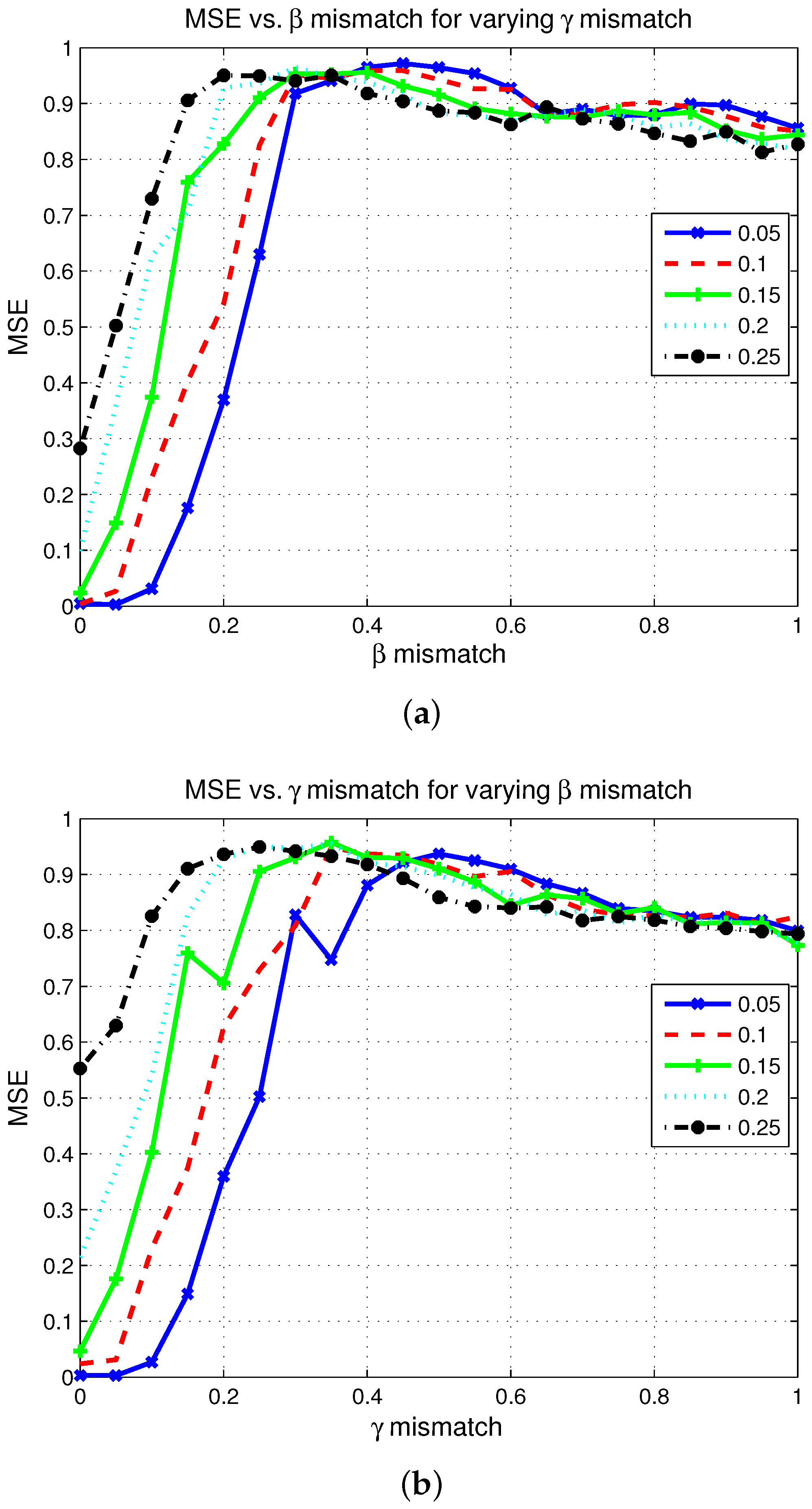
3.2. CS ISAR Dictionary Performance in Terms of Dictionary Mismatch

The performance of a fixed dictionary-based OMP reconstruction is dependent on the presence of a dictionary element with motion parameters close to the actual motion parameters. Failing that, the CS reconstruction may either not work at all or will lead to shifted and amplitude-degraded results. In the following, we consider factors affecting CS ISAR reconstruction performance when the dictionary contains third-order motion phase terms. We represent the correlation of two dictionary elements with mismatches in rotational rate, rotational acceleration and the rate of rotational acceleration as $\Delta \alpha ,\Delta \beta$ and $\Delta \gamma$, respectively. For the ease of analysis, we define the approximate linearized phase version of linear and quadratic chirps generated due to $\Delta \beta$ and $\Delta \gamma$ as follows:

$$exp(-j\Delta \beta {\tau }^2)\approx exp(-j{\alpha }_{\beta }\tau )$$

(29)

and:

$$exp(-j\Delta \gamma {\tau }^3)\approx exp(-j{\alpha }_{\gamma }\tau )$$

(30)

where ${\alpha }_{\beta }=\Delta \beta T_{\tau }$ and ${\alpha }_{\gamma }=\Delta \gamma T_{\tau }^2$ can be described as equivalent linear phase terms for the approximation. These phase terms are calculated by ensuring that the highest frequencies in the linearized phase versions are the same as in the original linear and quadratic phase terms. We consider four performance cases as follows.

3.2.1. Performance with Small $\Delta \gamma$ Mismatch

Consider the result of the correlation of a term $exp(j{\alpha }_1\tau +j{\beta }_1{\tau }^2+j{\gamma }_1{\tau }^3)$ in the received data and $exp(j{\alpha }_1\tau +j{\beta }_1{\tau }^2+j{\gamma }_2{\tau }^3)$ in the dictionary, where $\Delta \gamma ={\gamma }_2-{\gamma }_1$ gives a mismatch in the third-order motion phase term. The result of correlation is carried out in OMP reconstruction:

$$\begin{array}{cc}|<exp(j{\alpha }_1\tau +j{\beta }_1{\tau }^2+j{\gamma }_1{\tau }^3),exp(-j{\alpha }_1\tau -j{\beta }_1{\tau }^2-j{\gamma }_2{\tau }^3)>|\hfill & =|<exp(-j\Delta \gamma {\tau }^3)>|\hfill \\ & =\left|{\sum }_{n=0}^{N_{\tau }-1}exp\left(-j\Delta \gamma n^3\frac{1}{f_{\tau }^3}\right)\right|\hfill \end{array}$$

that can be approximated by making use of Equation (30) as follows:

$$\left|\sum _{n=0}^{N_{\tau }-1}exp\left(-j{\alpha }_{\gamma }n\frac{1}{f_{\tau }}\right)\right|$$

(31)

Considering $d_{\gamma }$ as the equivalent pixel shift arising due to the linearized version of the mismatch in γ denoted as ${\alpha }_{\gamma }$, we can describe it as:

$${\alpha }_{\gamma }=2\pi \Delta f{d}_{\gamma }$$

(32)

Subsequently, we can rewrite Equation (31) as:

$$\left|\sum _{n=0}^{N_{\tau }-1}exp\left(-j2\pi \Delta f{d}_{\gamma }\frac{n}{f_{\tau }}\right)\right|$$

(33)

When $d_{\gamma }=0$, the correlation would be a maximum, meaning that the received data component is matched to the dictionary element. This would lead to correct identification of the signal’s amplitude. The summation above can be further written as:

$$\left|N_{\tau }\mathrm{sinc}\left(N_{\tau }\pi \frac{\Delta f{d}_{\gamma }}{f_{\tau }}\right)\right|$$

(34)

This means that a mismatch of $\Delta \gamma$ effectively results in amplitude degradation of the estimated reflectivity as evident from the sinc term, with the estimated amplitude equal to zero when $d_{\gamma }$ is equal to $\overline{d}$ as follows:

$$\overline{d}=\frac{f_{\tau }}{N_{\tau }\Delta f}=\frac{1}{T_{\tau }\Delta f}$$

(35)

In order to reach the expression of $\Delta \gamma =\overline{\Delta \gamma }$ that causes this pixel shift $\overline{d}$ and, hence, a null estimated amplitude, we use the relationship given in Equation (32) and substitute $d_{\gamma }$ by $\overline{d}$ and ${\alpha }_{\gamma }$ by $\overline{\Delta \gamma }{T}_{\tau }^2$ in Equation (32) to get:

$$\overline{\Delta \gamma }{T}_{\tau }^2=\frac{2\pi }{T_{\tau }}$$

(36)

that leads to:

$$\overline{\Delta \gamma }=\frac{2\pi }{T_{\tau }^3}$$

(37)

A correlation of zero when the mismatch $\Delta \gamma =\overline{\Delta \gamma }$ would lead to arbitrary selection of a dictionary element and possibly lack of convergence of the OMP algorithm if ${\parallel \mathbf{\Delta }\mathit{s}\parallel }_2^2$ would not decrease after many repetitions. Therefore, the spacing of the rotational acceleration rate in the dictionary should be less than $\overline{\Delta \gamma }$. The case where this spacing is greater than $\overline{\Delta \gamma }$ is considered next.

3.2.2. Performance with Large $\Delta \gamma$ Mismatch

Consider the case of dictionary elements with rotational acceleration rate spacing greater than the limit of $\overline{\Delta \gamma }$. In this case, the result of correlation in Equation (34) will be very low. Assuming a mismatch in the rotational acceleration phase of $\Delta \gamma ={\gamma }_2-{\gamma }_1$ between two dictionary elements, such that these dictionary elements have rotational phases of ${\alpha }_1$ and ${\alpha }_2$ with $\Delta \alpha ={\alpha }_2-{\alpha }_1$, the correlation result for these two dictionary elements would be:

$$|<exp(-j\Delta \alpha \tau -j\Delta \gamma {\tau }^3)>|=|<exp(-j\Delta \alpha \tau -j{\alpha }_{\gamma }\tau )>|$$

The result of this correlation would be a maximum, when $\Delta \alpha +{\alpha }_{\gamma }=0$ or $\Delta \alpha =-{\alpha }_{\gamma }$, which means that when the dictionary is mismatched to the received data by $\Delta \alpha$ and $\Delta \gamma$, the reconstructed point should be at a location shifted by $d_{\alpha ,\gamma }$ from its original location and very low amplitude degradations, where:

$$d_{\alpha ,\gamma }=\frac{{\alpha }_{\gamma }}{2\pi \Delta f}$$

(38)

or:

$$d_{\alpha ,\gamma }=\frac{\Delta \gamma T_{\tau }^2}{2\pi \Delta f}$$

(39)

can be obtained from Equation (32).

When $\Delta \alpha \ne -{\alpha }_{\gamma }$, using $d_{\alpha ,\gamma }$ in lieu of $d_{\gamma }$ in Equation (34), the result of the correlation in Equation (38) would lead to an amplitude loss given as:

$$\left|N_{\tau }\mathrm{sinc}\left(N_{\tau }\pi \frac{\Delta f\mathrm{rem}(d_{\alpha ,\gamma }/\overline{d})}{f_{\tau }}\right)\right|$$

(40)

and a pixel-level position shift given as $\mathrm{int}(d_{\alpha ,\gamma }/\overline{d})$. The pixel-level position shift means that the detected position of a scatterer will not be at the original azimuth frequency bin, but at another azimuth frequency bin. The function $\mathrm{rem}(a/b)$ defines the remainder term when a is divided by b, and $\mathrm{int}(a/b)$ defines the integer part of the results of a divided by b. This means that we get a shift in position that gets larger with $d_{\alpha ,\gamma }$ and an amplitude degradation that get larger as the non-integer part of ${\displaystyle \frac{d_{\alpha ,\gamma }}{\overline{d}}}$ gets larger.

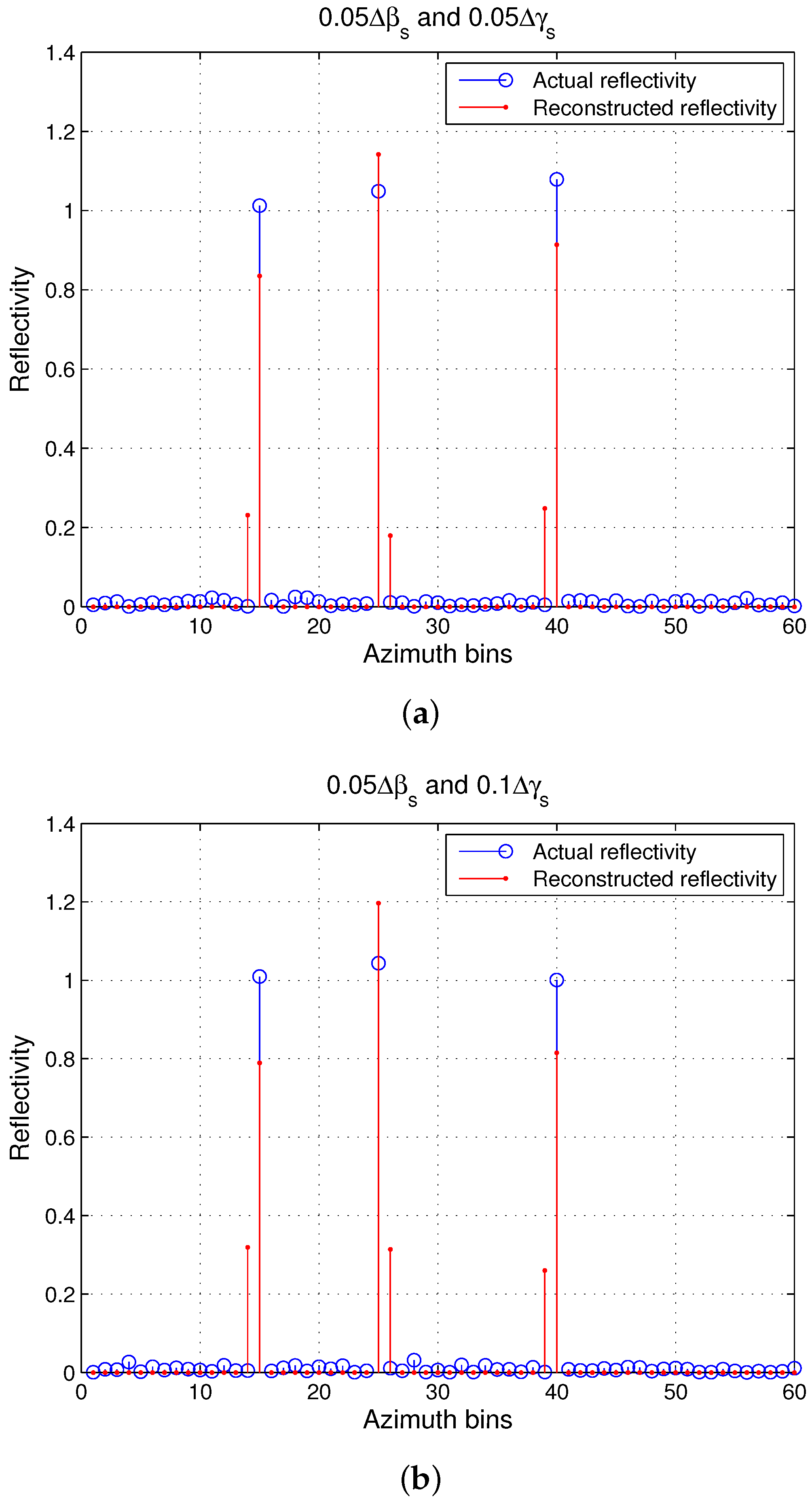
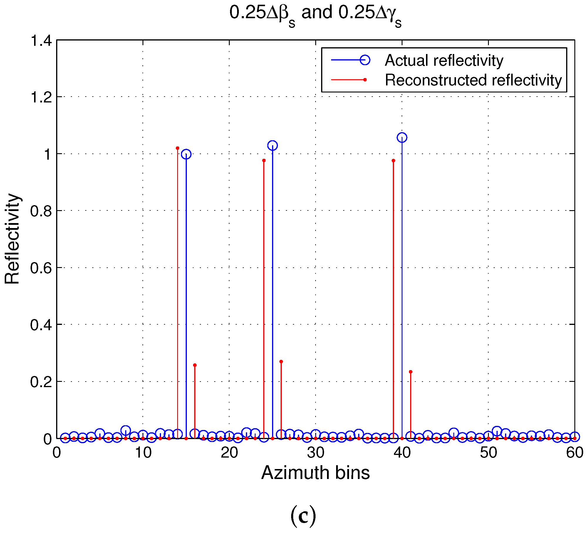
3.2.3. Performance with Small $\Delta \beta$ and $\Delta \gamma$ Mismatches

Consider the correlation of two elements mismatched in rotational acceleration and rotational acceleration rate by $\Delta \beta ={\beta }_2-{\beta }_1$ and $\Delta \gamma ={\gamma }_2-{\gamma }_1$, respectively. In this case, the correlation result would be:

$$|<exp(-j\Delta \beta {\tau }^2-j\Delta \gamma {\tau }^3)>|=|<exp(-j{\alpha }_{\beta }\tau -j{\alpha }_{\gamma }\tau )>|$$

(41)

When ${\alpha }_{\beta }=-{\alpha }_{\gamma }$, the result above would be a maximum, meaning that in such a case, the estimated position of the point would be the correct one as the mismatch due to $\Delta \beta$ is offset by the mismatch $-\Delta \gamma$. When ${\alpha }_{\beta }\ne -{\alpha }_{\gamma }$, the result would be degraded in amplitude, given by:

$$\left|N_{\tau }\mathrm{sinc}\left(N_{\tau }\pi \frac{\Delta f\mathrm{rem}(d_{\beta ,\gamma }/\overline{d})}{f_{\tau }}\right)\right|$$

(42)

where $d_{\beta ,\gamma }$ is a shift caused by $\Delta \beta$ and $\Delta \gamma$ described as follows:

$$2\pi \Delta f{d}_{\beta ,\gamma }={\alpha }_{\beta }+{\alpha }_{\gamma }=\Delta \beta T_{\tau }+\Delta \gamma T_{\tau }^2$$

(43)

or

$$d_{\beta ,\gamma }=\frac{\Delta \beta T_{\tau }+\Delta \gamma T_{\tau }^2}{2\pi \Delta f}$$

(44)

In order to avoid amplitude degradation, $d_{\beta ,\gamma }<\overline{d}$, which, making use of Equation (35), gives:

$$\Delta \beta T_{\tau }+\Delta \gamma T_{\tau }^2<\frac{2\pi }{T_{\tau }}$$

(45)

Note that this means that the constraints on spacing in β and γ are generally more strict when there is a mismatch in both of these parameters, as any mismatch in one parameter can cause reconstruction error, which would require the mismatch in the other parameter to be very small so as not to augment the overall reconstruction error. As an example, if $\Delta \gamma =0$, $\Delta \beta <\frac{2\pi }{T_{\tau }^2}$. If $\Delta \gamma =\frac{\pi }{T_{\tau }^3}$, then $\Delta \beta <\frac{\pi }{T_{\tau }^2}$. The next case shows the effects when the condition given by Equation (45) is not fulfilled.

3.2.4. Performance with Large $\Delta \beta$ and $\Delta \gamma$ Mismatches

Consider the case where there is mismatch $\Delta \beta ={\beta }_2-{\beta }_1$ and $\Delta \gamma ={\gamma }_2-{\gamma }_1$ between two dictionary elements, such that Equation (45) is not satisfied. These two dictionary elements further differ in rotational phase by $\Delta \alpha ={\alpha }_2-{\alpha }_1$. In this case, the correlation results would be:

$$|<exp(-j\Delta \alpha \tau -j\Delta \beta {\tau }^2-j\Delta \gamma {\tau }^3)>|=|<exp(-j\Delta \alpha \tau -j{\alpha }_{\beta }\tau -j{\alpha }_{\gamma }\tau )>|$$

(46)

The result of this correlation would be a maximum, when:

$$\Delta \alpha =-({\alpha }_{\beta }+{\alpha }_{\gamma })$$

(47)

which means that the estimated position would be shifted by $d_{\alpha ,\beta ,\gamma }$ pixels with almost no amplitude degradations, where:

$$2\pi \Delta f{d}_{\alpha ,\beta ,\gamma }={\alpha }_{\beta }+{\alpha }_{\gamma }=\Delta \beta T_{\tau }+\Delta \gamma T_{\tau }^2$$

(48)

or:

$$d_{\alpha ,\beta ,\gamma }=\frac{\Delta \beta T_{\tau }+\Delta \gamma T_{\tau }^2}{2\pi \Delta f}$$

(49)

When $\Delta \alpha \ne -({\alpha }_{\beta }+{\alpha }_{\gamma })$, the estimated amplitude would be degraded by:

$$\left|N_{\tau }\mathrm{sinc}\left(N_{\tau }\pi \frac{\Delta f\mathrm{rem}(d_{\alpha ,\beta ,\gamma }/\overline{d})}{f_{\tau }}\right)\right|$$

(50)

and shifted in position given by $\mathrm{int}(d_{\alpha ,\beta ,\gamma }/\overline{d})$. Note that the shifts in position are mainly there due to the mismatches $\Delta \beta$ and $\Delta \gamma$. Even if the rotation rate in the dictionary is perfectly matched to the rotation rate in the received data, the position shifts would occur because a dictionary element with another rotation rate gives the maximum correlation value due to the effects of $\Delta \beta$ and $\Delta \gamma$.

Table 1. Summary of dictionary performance. A × indicates the absence of mismatch, and a ✔ indicates the presence of mismatch.

Mismatch	$\mathbf{\Delta }\mathit{\alpha }$	$\mathbf{\Delta }\mathit{\beta }$	$\mathit{\Delta }\mathit{\gamma }$	Effects
Case 1	×	×	✔	Amplitude degradation if $\Delta \gamma$ is close to $\overline{\Delta \gamma }$.
Case 2	✔	×	✔	Amplitude degradation and position shift if $\Delta \gamma >\overline{\Delta \gamma }$ and $\Delta \alpha \ne -\Delta \gamma T_{\tau }^2$. Position shift only if $\Delta \alpha =\Delta \gamma T_{\tau }^2$.
Case 3	×	✔	✔	No position shift if $\Delta \beta =-\Delta \gamma T_{\tau }$. Otherwise, amplitude degradation and position shift.
Case 4	✔	✔	✔	Amplitude degradation and position shift if $\Delta \alpha \ne -(\Delta \beta T_{\tau }+\Delta \gamma T_{\tau }^2)$. Otherwise, position shift only.

summarizes and concludes the previous discussion on the dictionary performance.

3.3. Modified OMP

The OMP requires $M\times N_{\alpha ,\beta ,\gamma }$ computations in each repetition, which increase with the number of points $N_{\alpha ,\beta ,\gamma }$ in the dictionary. As shown in the previous section, the presence of mismatch in both rotational acceleration and rotational acceleration rate would require very fine parameter spacing that will increase the number of points leading to a large dictionary. In addition, a change in parameters would require the creation of a new dictionary each time the change occurs. Instead of making a very large dictionary, we propose a modification of the reconstruction problem based on a parametric dictionary. This means that the dictionary is not fixed, but is calculated as a function of different motion parameters. In this case, this minimization problem for CS ISAR reconstruction can be written as:

$$\widehat{\mathit{\sigma }}(\widehat{\mathit{\alpha }},\widehat{\mathit{\beta }},\widehat{\mathit{\gamma }})=\underset{\mathit{\sigma },\mathit{\alpha },\mathit{\beta },\mathit{\gamma }}{\mathrm{argmin}}\parallel \mathit{s}-\mathsf{\Phi }\mathsf{\Psi }(\mathit{\alpha },\mathit{\beta },\mathit{\gamma }){\mathit{\sigma }\parallel }_2^2+\lambda {\parallel \mathit{\sigma }\parallel }_0$$

(51)

The term $\mathsf{\Psi }(\mathit{\alpha },\mathit{\beta },\mathit{\gamma })$ shows the dictionary to be varying with the values of rotation rate phase terms α, rotational acceleration phase terms β and rotational acceleration rate phase terms γ that are calculated by solving the minimization problem. The reconstruction can be carried out with a modification of Step 2 of the OMP algorithm to the following constrained optimization problem:

$$\underset{\mathit{\psi }({\alpha }_k,{\beta }_k,{\gamma }_k)}{\mathrm{argmin}}\frac{\left|\right|\mathit{s}-[\mathbf{\Delta }\mathsf{\Psi },(\mathsf{\Phi }\mathit{\psi }({\alpha }_k,{\beta }_k,{\gamma }_k))]{\widehat{\mathit{\sigma }}}_k{\left|\right|}_2^2}{{\left|\right|\mathit{s}\left|\right|}_2^2}$$

(52)

subject to:

$$\begin{array}{c}C1:\mathit{\psi }({\alpha }_k,{\beta }_k,{\gamma }_k)=\mathrm{rect}\left(\frac{\tau }{T_{\tau }}\right)exp\left(-j{\alpha }_k\tau -j{\beta }_k{\tau }^2-j{\gamma }_k{\tau }^3\right)\hfill \\ C2:{\alpha }_{min}\le {\alpha }_k\le {\alpha }_{max}\hfill \\ C3:{\beta }_{min}\le {\beta }_k\le {\beta }_{max}\hfill \\ C4:{\gamma }_{min}\le {\gamma }_k\le {\gamma }_{max}\hfill \\ C5:{\widehat{\mathit{\sigma }}}_k=\underset{\mathit{\sigma }}{\mathrm{argmin}}\left|\right|\mathit{s}-[\mathbf{\Delta }\mathsf{\Psi },(\mathsf{\Phi }\mathit{\psi }({\alpha }_k,{\beta }_k,{\gamma }_k))]\mathit{\sigma }{\left|\right|}_2^2\hfill \end{array}$$

(53)

where ${\alpha }_{min},{\alpha }_{max},{\beta }_{min},{\beta }_{max},{\gamma }_{min}$ and ${\gamma }_{max}$ are the maximum and minimum limits of these parameters. The constraint $C1$ ensures that the selected dictionary element is a function of the parameters given by ${\alpha }_k,{\beta }_k$ and ${\gamma }_k$. The constraints $C2$, $C3$ and $C4$ ensure that the values of ${\alpha }_k$, ${\beta }_k$ and ${\gamma }_k$ used to generate the dictionary elements are within the minimum and maximum limits specified. The constraint $C5$ ensures that the ${\widehat{\mathit{\sigma }}}_k$ used in the objective function is a least-squares solution using the selected dictionary element, as in Step 4 of the OMP algorithm.

Step 3 of the OMP algorithm is also modified as:

$$\mathbf{\Delta }\mathsf{\Psi }=[\Delta \mathsf{\Psi },\mathsf{\Phi }\mathit{\psi }({\alpha }_k,{\beta }_k,{\gamma }_k)]$$

(54)

The optimization problem above estimates the motion parameters, and the objective function ensures that the ratio $\frac{{\parallel \mathbf{\Delta }\mathit{s}\parallel }_2^2}{{\parallel \mathit{s}\parallel }_2^2}$ at each repetition is as small as possible, ensuring that the selected values of the motion parameters are as close as possible to the actual parameters in the data. The proposed modification does not require the creation of a dictionary. The optimization problem can be solved using an algorithm, such as the Genetic Algorithm (GA) [42], because GA can generally arrive at a global solution to an optimization problem. We call this algorithm GA-based OMP (GAOMP). Note that our proposed algorithm is not specifically dependent on GA, and another global optimization algorithm can also be used.

The GAOMP may suffer from inaccuracies due to a huge search space for the three motion parameters. In order to reduce the search space, we propose a further modification to the above algorithm, where we assume that the positions either lie on a given or an upsampled grid. The new modification can be seen as a hybrid fixed dictionary based on positions and a parametric dictionary based on rotational acceleration and rotational acceleration rate. The assumption of positions represented by a given grid is practical as, due to a relatively small extent size of an ISAR imaged scene, an upsampling of azimuth position parameters can be carried out without requiring any significant computations or space. In addition, unlike a fixed dictionary, creating dictionary elements with rotational acceleration and rotational acceleration rate parameters having very fine spacing is not required, which results in eventual saving of space and computations. The new modified algorithm is as follows:

$$\underset{{\mathit{\psi }}^i({\beta }_k,{\gamma }_k)}{\mathrm{argmin}}\frac{\left|\right|\mathit{s}-[\mathbf{\Delta }\mathsf{\Psi },(\mathsf{\Phi }{\mathit{\psi }}^i({\beta }_k,{\gamma }_k))]{\widehat{\mathit{\sigma }}}_i^k{\left|\right|}_2^2}{{\left|\right|\mathit{s}\left|\right|}_2^2}$$

(55)

subject to

$$\begin{array}{cc}C1:& {\mathit{\psi }}^1({\beta }_k,{\gamma }_k)=\mathrm{rect}\left(\frac{\tau }{T_{\tau }}\right)exp\left(-j{\alpha }_1\tau -j{\beta }_k{\tau }^2-j{\gamma }_k{\tau }^3\right)\hfill \\ & {\mathit{\psi }}^2({\beta }_k,{\gamma }_k)=\mathrm{rect}\left(\frac{\tau }{T_{\tau }}\right)exp\left(-j{\alpha }_2\tau -j{\beta }_k{\tau }^2-j{\gamma }_k{\tau }^3\right)\hfill \\ & .\hfill \\ & .\hfill \\ & .\hfill \\ & {\mathit{\psi }}^{N_{\alpha }}({\beta }_k,{\gamma }_k)=\mathrm{rect}\left(\frac{\tau }{T_{\tau }}\right)exp\left(-j{\alpha }_{N_{\alpha }}\tau -j{\beta }_k{\tau }^2-j{\gamma }_k{\tau }^3\right)\hfill \\ C2:& {\alpha }_i=\frac{(i-1)({\alpha }_{max}-{\alpha }_{min})}{N_{\alpha }},1\le i\le N_{\alpha }\hfill \\ C3:& {\beta }_{min}\le {\beta }_k\le {\beta }_{max}\hfill \\ C4:& {\gamma }_{min}\le {\gamma }_k\le {\gamma }_{max}\hfill \\ C5:& {\widehat{\mathit{\sigma }}}_k^i=\underset{{\mathit{\sigma }}^i}{\mathrm{argmin}}\left|\right|\mathit{s}-[\mathbf{\Delta }\mathsf{\Psi },(\mathsf{\Phi }{\mathit{\psi }}^i({\beta }_k,{\gamma }_k))]{\mathit{\sigma }}^i{\left|\right|}_2^2,1\le i\le N_{\alpha }\hfill \end{array}$$

and:

$$\mathbf{\Delta }\mathsf{\Psi }=[\Delta \mathsf{\Psi },\mathsf{\Phi }{\mathit{\psi }}^i({\beta }_k,{\gamma }_k)]$$

(56)

The constraint $C1$ ensures that each dictionary element is a function of the given set of positions represented by ${\alpha }_i$. The constraint $C2$ ensures that the ${\alpha }_i$ values used are from the values specified. The constraints $C3-C5$ are similar to those given in GAOMP. This step reduces the search space, as now, the search will be on parameters β and γ only, for all of the given grid parameters. We call this modified algorithm Dictionary-based GAOMP (DGAOMP).

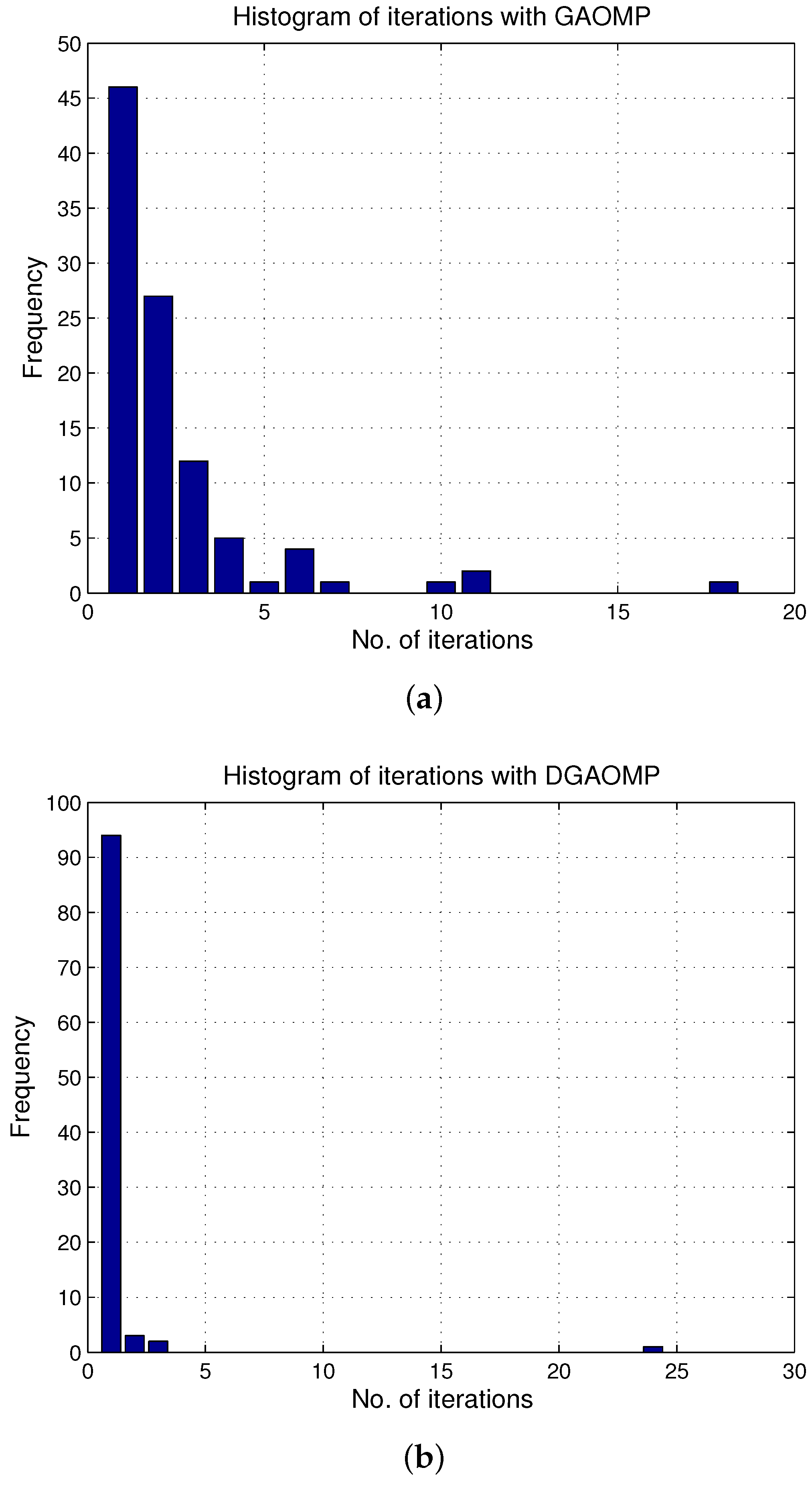
3.4. Computational Complexity

GA repeatedly generates a number of solutions, denoted by $N_p$. At each generation of $N_p$ solutions, the objective function is evaluated with these solutions, and solutions deemed as better are selected to produce another set of $N_p$ solutions. This is continued for a total number of generations $N_g$. In order to calculate the complexity, we consider the total number of evaluations of the objective function at the k-th repetition. As the objective function consists of a least-squares solution, its computational complexity is given by $M{k}^2$. For DGAOMP, this evaluation is carried out for $N_{\alpha }$ values, resulting in a computational complexity of $M{k}^2{N}_{\alpha }$. As there are $N_p$ solutions and $N_g$ generations, the total computational complexity becomes $M{k}^2{N}_{\alpha }{N}_p{N}_g$. A dictionary-based approach mainly consists of calculating the correlation of the data with each dictionary element, which results in a computational complexity of $M{N}_{\alpha }{N}_{\beta }{N}_{\gamma }$ at each iteration. In our simulations, $N_p$ is 20, and the maximum $N_g$ is 200. As $N_{\beta }$ and $N_{\gamma }$ are of the order of a few thousand and a few hundred samples, respectively for fine spacing of β and γ parameters, the overall computational complexity for DGAOMP is less than a fixed dictionary based on finely-sampled motion parameters. This computational complexity will increase as the number of repetitions increases; however, due to the sparsity of the imaged scene, the maximum number of repetitions will be low, which means that DGAOMP will retain its advantage of lower computational complexity. For the sake of comparison, we mention the computational complexity of GAOMP, which is $M{k}^2{N}_p{N}_g$ and less than DGAOMP. In the next section, we show that the DGAOMP gives lower reconstruction error compared to the GAOMP, which is at the expense of a higher number of computations involved in the former algorithm.

4. Results

In this section, we first present ISAR image reconstruction results in the range azimuth frequency domain with DGAOMP and compare with existing methods. Then, we present numerical results that show the effects of the level of mismatch in rotational acceleration and rotational acceleration rate on a fixed dictionary performance, further motivating the use of DGAOMP. In the end, we present quantitative results demonstrating the performance of the proposed algorithm.

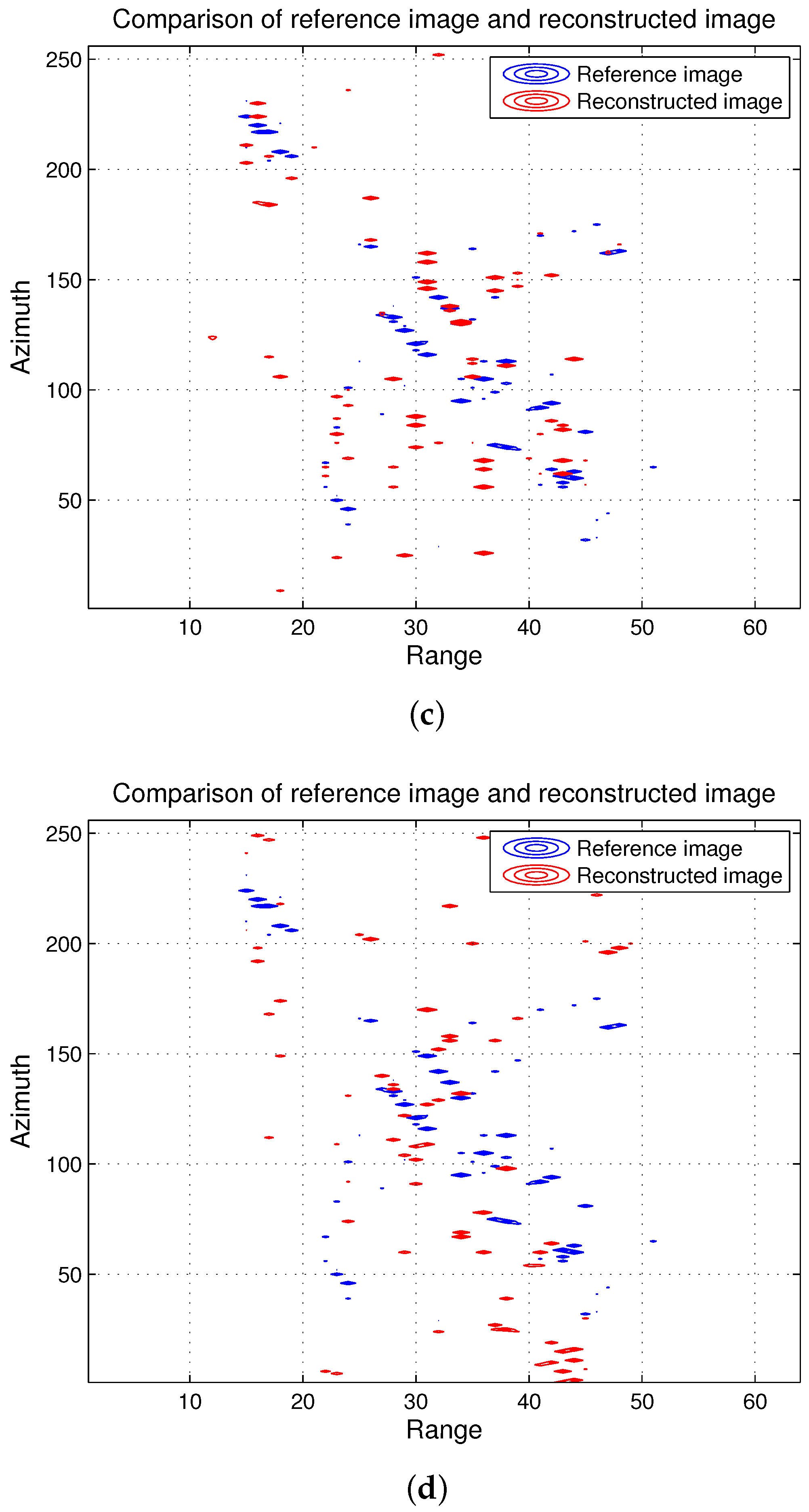
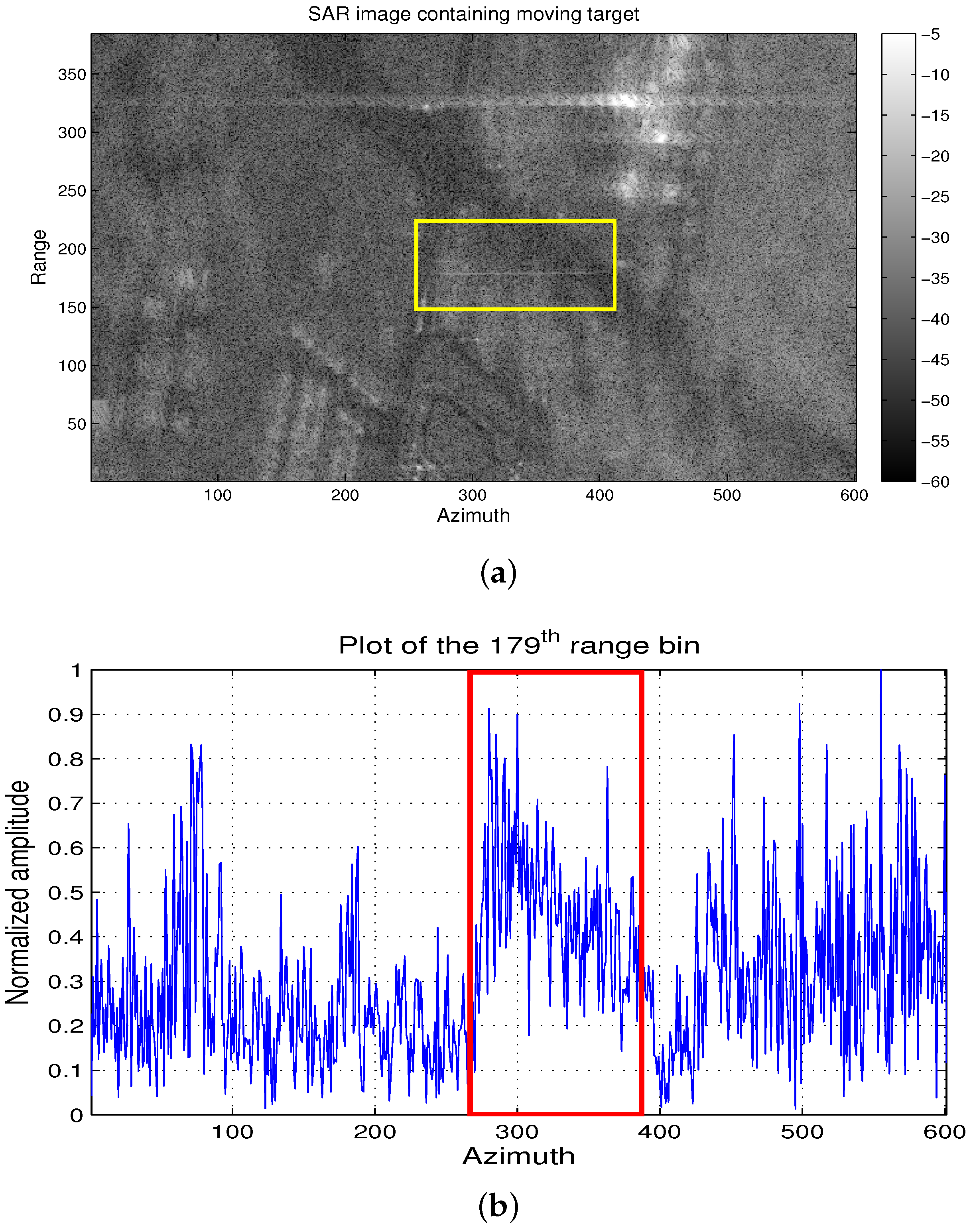
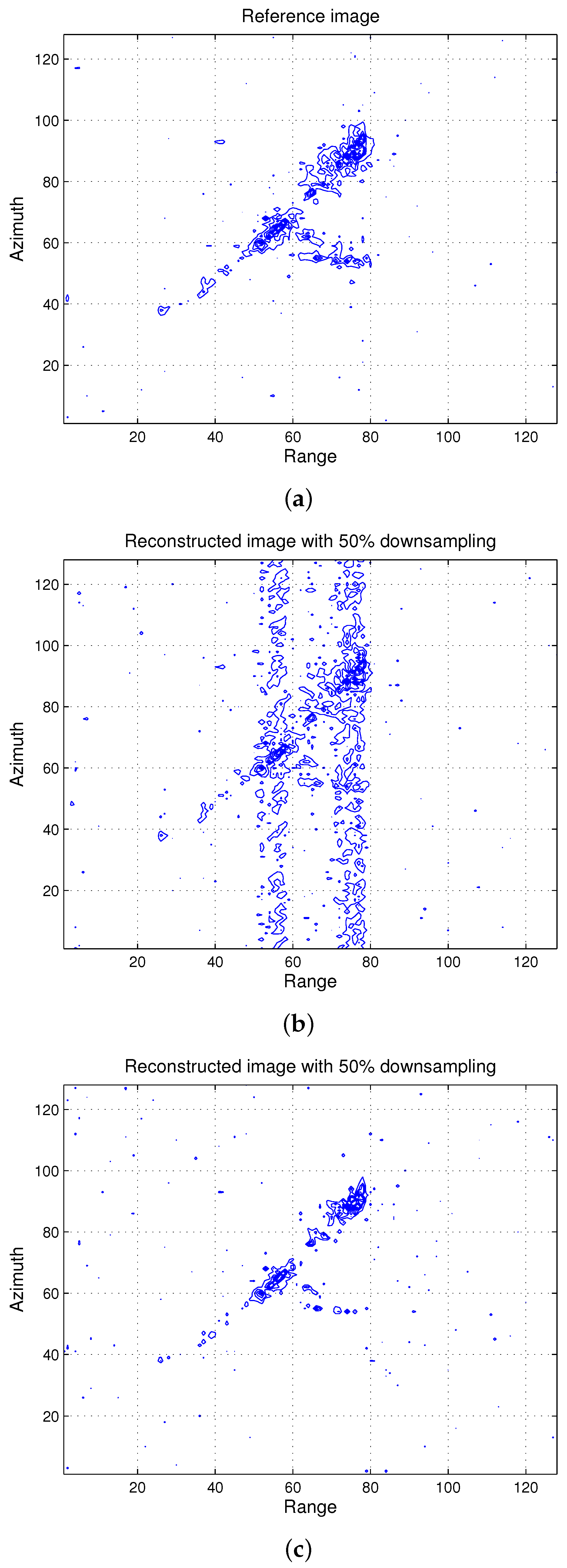
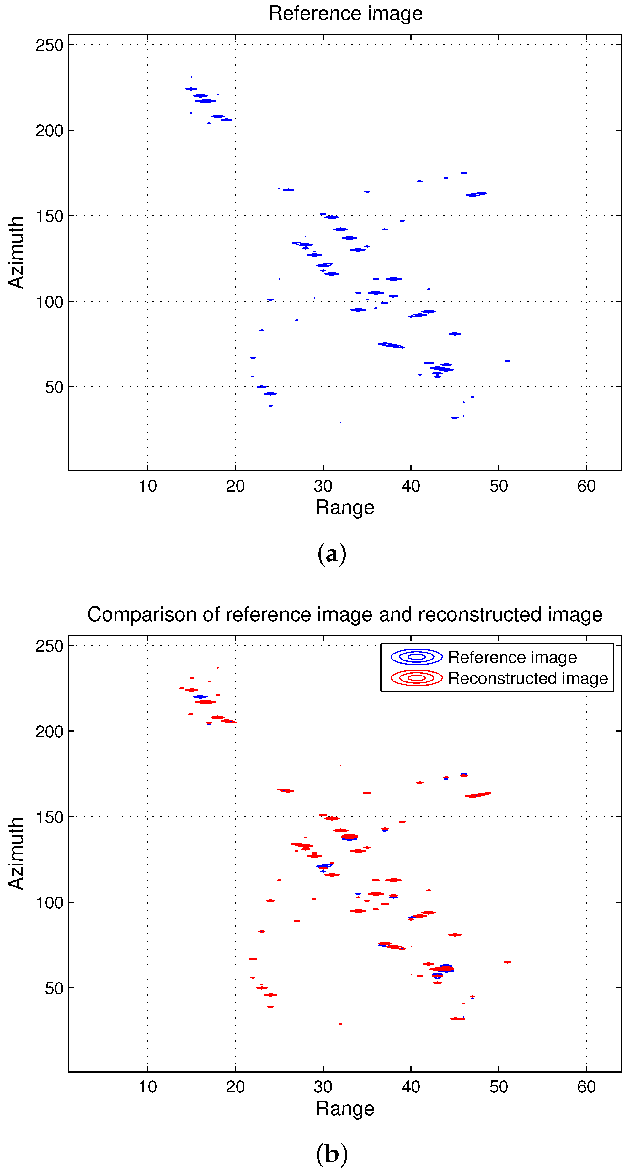
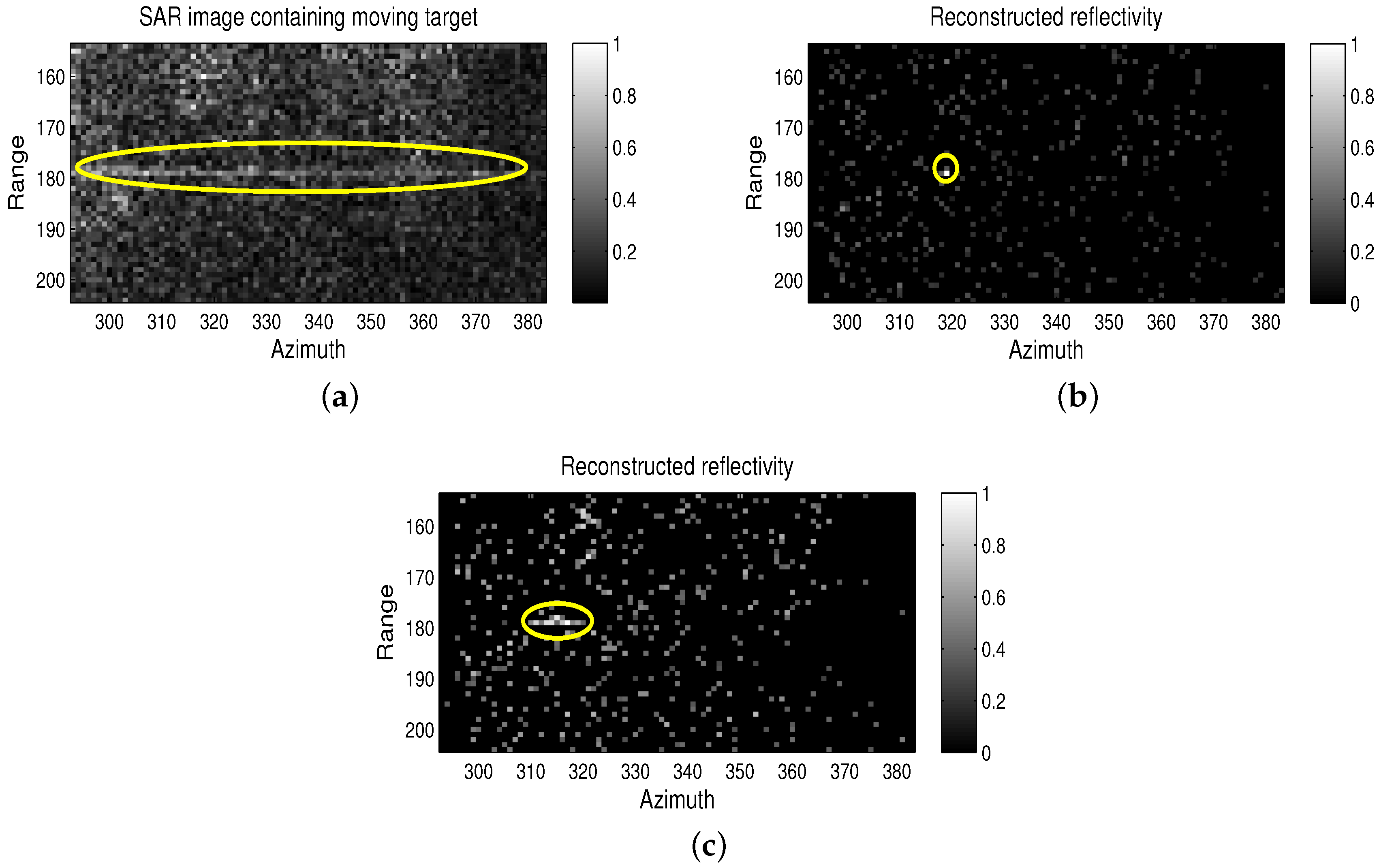
4.1. Imaging Results

In this section, we first show the applicability of the proposed technique to real ISAR data used in [36]. The data consist of an equal number of 128 range and azimuth bins and require an FT to get the focused image, as shown in Figure 1a. The result of using FT on data randomly downsampled by $50\%$ in the azimuth direction is shown in Figure 1b. As can be seen, the resulting image suffers from artifacts due to aliasing. Next, we apply the proposed technique to the downsampled data. As the data do not contain any rotational acceleration or rate of change of rotational acceleration, the reconstruction consists of estimating the azimuth frequency of scatterers and reflectivity in each range bin. Figure 1c shows the focused image without any artifacts seen in Figure 1b that serves as evidence of the applicability of our proposed method to real ISAR data.

The next set of figures shows the performance of the proposed method on 2D simulated ISAR data used in [36]. The reflectivity of the original image is shown in Figure 2a, and random rotational acceleration and rotational acceleration rates were assigned to different scatterers. The number of range and azimuth bins were 64 and 256, respectively. The reconstructed image using GAOMP overlapped with the reference image is shown in Figure 2b. As can be seen, the reconstruction positions the scatterers on their correct locations for a large majority of the scatterers, which confirms the ability of DGAOMP to carry out CS ISAR imaging.

Next, we compare the reconstruction performance using an existing technique [26] that can image fully-sampled CS ISAR data having high maneuverable motion. The technique uses an integrated high-order matched phase transform that processes fully-sampled ISAR data with motion having a rotational acceleration rate component. When $50\%$ of the randomly downsampled data are used for reconstruction, we can note in Figure 2c that only a few scatterers are positioned correctly, as the aforementioned method requires complete data.

Figure 2d further shows the reconstruction result using a dictionary that only consists of rotation rate and rotational acceleration, as is the case with a few existing CS ISAR imaging techniques mentioned in Section 1. It can be seen that the reconstruction fails to form the image correctly, which emphasizes the fact that existing CS ISAR imaging methods that approximate rotational motion till a rotational acceleration term cannot image data having highly maneuvering motion, unlike the technique proposed in this report.

Our final example with the Gotcha GMTIdataset, described in [43] and available on [44], further demonstrates the applicability of the proposed DGAOMP algorithm to real data. Part of the data corresponding to the starting time of 6.9 seconds and consisting of 386 range samples and 3728 azimuth samples was selected. The sampling frequency of the data is 2172 Hz. A slice of the image formed by FT of the raw data is shown in Figure 3a, where a defocused object within the indicated rectangle is visible. This object is actually a vehicle, and its static image will be concentrated only around a few pixels, unlike the defocused image, where it is spread over many pixels. The spread is caused by the motion of a vehicle that causes the appearance of first-, second- and third-order phase terms in the raw data [45]. The imaging relation between the image and the raw data is represented by FT and, hence, is similar to the ISAR configuration that we dealt with in the preceding examples.

Figure 3b shows the data selected from range bin No. 179 normalized by the maximum amplitude of the raw data. The azimuth bins containing the defocused object were selected, as shown by the rectangle. The inverse FT of the selected azimuth bins was used to go back to the raw data containing the phase history of the moving object. The raw data randomly downsampled by 50% were then processed by DGAOMP; the number of iterations were limited to eight, as no significant decrease in the value of $\frac{{\parallel \mathbf{\Delta }\mathit{s}\parallel }_2^2}{{\parallel \mathit{s}\parallel }_2^2}$ was noted after eight iterations. The values of ${\beta }_{min}$, ${\beta }_{max}$, ${\gamma }_{min}$ and ${\gamma }_{max}$ were fixed as −625 Hz/s, 625 Hz/s, −625 Hz/${\mathrm{s}}^2$ and 625 Hz/${\mathrm{s}}^2$, as the solution provided by the DGAOMP always stayed within these values for the selected dataset. The final value of $\frac{{\parallel \mathbf{\Delta }\mathit{s}\parallel }_2^2}{{\parallel \mathit{s}\parallel }_2^2}$ was around 0.1. The resulting reflectivity estimate is shown in Figure 3c. Compared to Figure 3b, it is evident that the defocusing caused by the motion has been eliminated, and a high peak and a few low peaks replace the defocused part and show a focused reflectivity. The reflectivity estimate with a limited motion model given by Equation (7), which ignores the acceleration rate, is shown in Figure 3d. It took eight iterations for the value of $\frac{{\parallel \mathbf{\Delta }\mathit{s}\parallel }_2^2}{{\parallel \mathit{s}\parallel }_2^2}$ to reach 0.2 with no further decrease, and as a result, a higher number of scattered peaks can be seen. The difference in amplitude between the highest peak and the lower peaks is less than that in Figure 3d. This confirms the applicability of the proposed algorithm to reconstruct reflectivity from real data containing unknown realistic motion.

We further show 2D processing results. The patch highlighted by the rectangle in Figure 3a was extracted and normalized by the highest amplitude value in the patch. It is shown in Figure 4a, where the ellipse highlights the defocusing caused by the target motion. Raw data corresponding to the patch were randomly downsampled by 50% and processed by DGAOMP. The resulting normalized image is shown in Figure 4b, where it can be seen that the moving target is focused in a very small area, highlighted by the circle. When the limited motion model in Equation (7) was used for processing the data, the resulting normalized image, although better focused compared to the image in Figure 3a, was still partially defocused, as shown in Figure 4c. Comparing Figure 4b,c, in the former figure, the target is more prominent compared to the background due to better focusing capability of DGAOMP using the third-order motion phase model. This further emphasizes the applicability of the motion model and DGAOMP for processing real data.

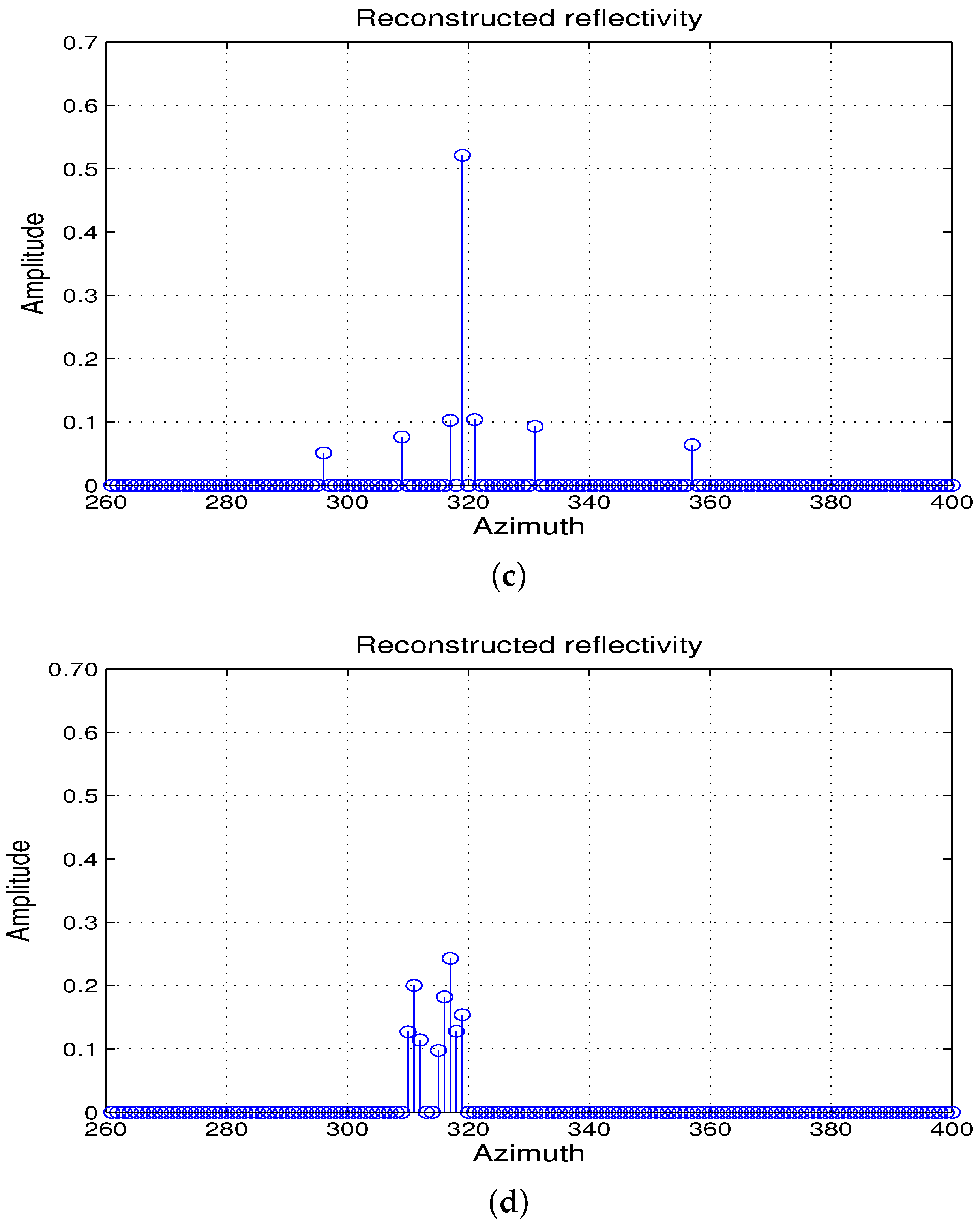
4.2. Numerical Results

We simulate 1D data according to the following parameters: $N_{\tau }=256$, which is the number of azimuth bins, azimuth pulse length $T_{\tau }=12.75$ ms, azimuth sampling frequency $f_s=20$ kHz, $\Delta f=78$ Hz and linear and quadratic chirp rates varying from −4.9 to 4.9 MHz/s and −61.5 to 61.5 $\mathrm{MHz}/{\mathrm{s}}^2$, respectively. A random downsampling of 50% was carried out for the data, and an Signal-to-Clutter Ratio (SCR) of 20 dB after downsampling was maintained. The scatterers could lie either on the azimuth bins or in between two azimuth bins.

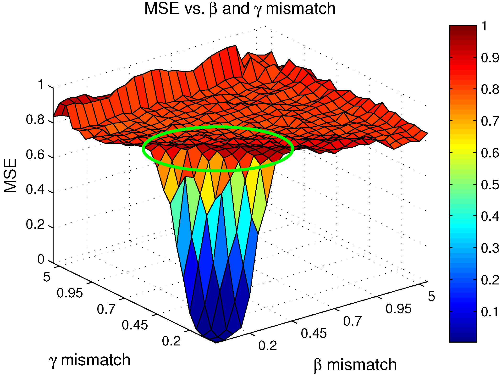
4.2.1. Performance of the CS ISAR Dictionary in the Presence of Mismatch

We first confirm the analysis carried out in Section 3.2 by generating data from a given dictionary and reconstructing in the azimuth frequency domain using mismatched dictionaries. The mismatch in rotational acceleration and rotational acceleration rate, henceforth referred to as β mismatch and γ mismatch, respectively, is carried out in step-sizes of $0.05\Delta {\beta }_s/\Delta {\gamma }_s$ from zero to $\Delta {\beta }_s/\Delta {\gamma }_s$ and then from $0.05\Delta {\beta }_s/\Delta {\gamma }_s$ to $5\Delta {\beta }_s/\Delta {\gamma }_s$ in step-sizes of $\Delta {\beta }_s/\Delta {\gamma }_s$. The step-size $\Delta {\beta }_s$ is 40 kHz/s, and $\Delta {\gamma }_s$ is 3 $\mathrm{MHz}/{\mathrm{s}}^2$. Figure 5a,b shows the MSE normalized with respect to the maximum MSE for varying values of β mismatch and γ mismatch. MSE was measured based on the estimated reflectivity and position compared to the actual reflectivity and position as follows:

$$MSE=\frac{{\sum }_{i=1}^{N_e}\left|\right|{\mathit{\sigma }}_i(\mathit{\alpha })-{\widehat{\mathit{\sigma }}}_i(\widehat{\mathit{\alpha }}){\left|\right|}_2^2}{N_{\alpha }{N}_e}$$

(57)

where ${\sigma }_i(\alpha )$ is the actual reflectivity, ${\widehat{\sigma }}_i(\widehat{\alpha })$ is the estimated reflectivity for the i-th experiment and $N_e$ is the total number of experiments. The MSE was normalized by the maximum MSE obtained among all of the experiments, which corresponds to the case where all of the reconstructed scatterers are misaligned and can also have sidelobes in the reconstruction.

In Figure 5a, we can see MSE versus β mismatch for varying values of γ mismatch. For the sake of clarity of presentation, we limit the values of β mismatch between zero and $\Delta {\beta }_s$ and those of γ mismatch between $0.05\Delta {\gamma }_s$ and $0.25\Delta {\gamma }_s$. As expected, the value of MSE increases and then becomes stable as the reconstructed points are totally shifted from the actual positions, and the error becomes maximum due to total misalignment of positions. The mismatch value at which the MSE becomes maximum decreases with an increasing γ mismatch, evidenced by the peak point of the MSE shifting towards left with increased mismatch.

Figure 5b gives the MSE versus γ mismatch for varying values of β mismatch. Similar to Figure 5a, we can see that MSE becomes roughly constant, and the value of the mismatch when the MSE becomes roughly constant is 1.5 $\mathrm{MHz}/{\mathrm{s}}^2$. Note that once the limit given by $\overline{\Delta \gamma }$ in Equation (37) is exceeded, the mismatch causes single or multiple position shifts from one azimuth frequency bin to another. As in our simulation, the scatterer can also lie in between two azimuth frequency bins, the limit will be halved, which is 1.5 $\mathrm{MHz}/{\mathrm{s}}^2$, conforming with the results in Figure 5b where the MSE becomes constant at 0.5$\Delta {\gamma }_s=1.5$$\mathrm{MHz}/{\mathrm{s}}^2$. It can be further seen that MSE increases when γ mismatch is fixed and β mismatch is increased. Furthermore, it can be noted compared to Figure 5b that the MSE is more sensitive to β mismatch as evidenced by a higher value of MSE for a β mismatch, compared to the same level of γ mismatch.

Figure 6 shows a complete 2D situation of MSE versus β mismatch and γ mismatch varying from zero to $5\Delta {\beta }_s/\Delta {\gamma }_s$. As outlined in Figure 5a,b, it can be seen that as the β mismatch increases, the MSE curve reaches the highest value with decreasing values of γ mismatch. This effect is highlighted by the encircled slanted error surface and requires finer spacing of parameters in the presence of both mismatches compared to mismatch of a single parameter, as described by Equation (45). As an example, if a dictionary is created with a spacing of $0.1\Delta {\beta }_s$ and $0.1\Delta {\gamma }_s$ to keep MSE around 0.2, it would lead to $N_{\beta }=2451$ and $N_{\gamma }=411$, requiring a dictionary with $N_{\beta }{N}_{\gamma }$ entries that are around a million entries. The ratio of the number of computations required by a fixed dictionary based on these values of $N_{\beta }$ and $N_{\gamma }$ to the number of computations required by DGAOMP with $N_p=20$ and $N_g=200$ will be around six times for ten iterations. The ratio will decrease as the number of iterations increases, reducing the advantage offered by DGAOMP; however, due to the sparse nature of the scenes being imaged, the number of iterations is low, as confirmed by the real SAR data, where the maximum number of iterations was eight.

We give a further example with different values of β mismatch and γ mismatch and their effects on the reconstruction image. First, we set β mismatch and γ mismatch to be 0.05$\Delta {\beta }_s$ and 0.05$\Delta {\gamma }_s$, respectively. The raw data simulated with randomly chosen positions, rotational acceleration and rate of change of rotational acceleration are reconstructed using a dictionary that has the mismatch specified previously. The sparsity is fixed at three, and the maximum number of repetitions of the OMP is set as six, to show the immediate sidelobes. The result is shown in Figure 7a. It can be seen that the scatterers are detected at their original positions, with almost the correct amplitude and a few sidelobes.

Next, the result with β mismatch and γ mismatch of 0.05$\Delta {\beta }_s$ and 0.1$\Delta {\gamma }_s$, respectively, is shown in Figure 7b. It can be seen that although the positions are detected correctly, the estimated amplitudes have a greater difference compared to the actual amplitude, and the sidelobes are higher. Finally, we show the result in Figure 7c when the β mismatch and γ mismatch are 0.25$\Delta {\beta }_s$ and 0.25$\Delta {\gamma }_s$, respectively. It can be seen that the reconstructed positions are shifted from the actual positions, and there are a few sidelobes in the vicinity. Note again that in the presence of mismatch in a single parameter, the pixel shift would have occurred at a higher value of mismatch, e.g., if there were only γ mismatch, the shift would have occurred at $0.5\Delta {\gamma }_s$. This emphasizes the necessity of using very fine parameter spacing when using a fixed dictionary and motivates the use of the parametric dictionary approach proposed in this report.

4.2.2. Reconstruction Performance of the Proposed Algorithm

We first show the convergence performance of GAOMP and DGAOMP techniques. Different sets of scatterers with sparsity equal to three with random positions, rotational acceleration and rate of rotational acceleration were simulated. Both techniques were applied to data simulated from these sets. The threshold υ was set as 0.03 because this is a reasonable number for the ratio of noise energy to raw data energy, when SNR = 20 dB. The number of repetitions K needed for the ratio $\frac{{\parallel \Delta \mathit{s}\parallel }_2^2}{{\parallel \mathit{s}\parallel }_2^2}$ to go below 0.03 was recorded. Ideally, the number of repetitions should be three, as that is the sparsity, and after three repetitions, the major part of the signal should be removed. Each time the number of repetitions exceeded three, the reconstruction algorithm was restarted. One iteration to reconstruct the data in one experiment was defined as consisting of three repetitions. The number of iterations for each dataset was recorded using both algorithms for a total number of a hundred experiments. Figure 8a,b shows the frequency for different iterations with both techniques. The GAOMP algorithm needed one iteration in approximately $45\%$ of the simulation cases, followed by a decreasing share of approximately $50\%$ of the simulation cases till five iterations. The remaining $5\%$ simulations are distributed between six, seven, ten, eleven and eighteen iterations. For DGAOMP, around $95\%$ of the simulations took one iteration for the ratio $\frac{{\parallel \Delta \mathit{s}\parallel }_2^2}{{\parallel \mathit{s}\parallel }_2^2}$ to go below 0.03, with the remaining simulations distributed between two, three and a single case of twenty-four iterations. This shows that among the two techniques, the DGAOMP technique can converge to a solution with higher probability.

A comparison of the performance of the two techniques with respect to a changing Signal-to-Clutter Ratio (SCR) was also made via Monte Carlo simulations, the results of which are shown in Figure 9a. Noise was added according to the scatterers’ reflectivity, such that the SCR after downsampling varied between 10 and 20 dB. The motion parameters for each scatterer were generated randomly, and the resulting data were processed by these techniques. The results in Figure 9a demonstrate that the reconstruction based on DGAOMP has lower MSE for all of the SCR values compared to the reconstruction based on GAOMP. The difference in MSE becomes significantly prominent for higher SCR values. For lower SCR, both techniques give erroneous results causing a higher MSE. The DGAOMP technique still shows slightly lower MSE thanks to the lower search space that is required to select one of the given grid positions, unlike GAOMP, which has to estimate the grid position in between the given limits. Based on Figure 8 and Figure 9a, it is clear that although both techniques can reconstruct compressively-sensed ISAR data, the DGAOMP technique performs better. Hence, we use it for subsequent performance evaluation.

Figure 9b shows the performance of DGAOMP reconstruction versus sparsity. The reconstruction algorithm’s iterations were fixed up to the sparsity level. It can be seen that MSE increases almost linearly with sparsity varying from one to seven. The reason is that the estimation of each scatterer’s amplitude leads to some error, and as a result, the error accumulates. The error becomes almost constant between 0.45 and 0.5 with sparsity greater than or equal to seven, as the algorithm reaches its limit for the number of scatterers that can be estimated correctly. This is consistent with the performance limit that describes the minimum number of measurements as $M\ge 3K{\log }_2{N}_{\tau }$, as well as Figure 9a, where for low SCR when the performance of DGAOMP degraded, the MSE was around 0.45.

5. Conclusions

In this report, we presented a new compressed sensing ISAR imaging algorithm in order to deal with the case of high maneuvering motion that consists of rotational acceleration rate. The algorithm first presented a new dictionary consisting of three phase terms arising due to rotation rate, rotational acceleration and rate of rotational acceleration. The dictionary can deal with high maneuvering motion. Analysis of the dictionary was carried out, which revealed that using a fixed dictionary would require very fine spacing of different parameters in the dictionary, leading to huge storage space and computational requirements. We proposed a modification where a parametric dictionary was used to estimate rotational acceleration and rate of rotational acceleration for a given grid as positions. The orthogonal matching pursuit algorithm was modified in order to carry out reconstruction with this parametric dictionary making use of the genetic algorithm to estimate rotational acceleration and rate of rotational acceleration. We presented numerical examples as a function of changing signal-to-clutter ratios and sparsity levels to show the performance of the proposed approach. Further imaging examples with compressively-sensed ISAR data showed the effectiveness of the proposed approach compared to existing approaches.

References

- Candès, E.; Tao, T. Near-optimal signal recovery from random projections: universal encoding strategies? IEEE Trans. Inf. Theory 2006, 52, 5406–5425. [Google Scholar] [CrossRef]
- Candès, E.; Romberg, J.; Tao, T. Robust uncertainty principles: Exact signal reconstruction from highly incomplete frequency information. IEEE Trans. Inf. Theory 2006, 52, 489–590. [Google Scholar] [CrossRef]
- Donoho, D. Compressed sensing. IEEE Trans. Inf. Theory 2006, 52, 1289–1306. [Google Scholar] [CrossRef]
- Baraniuk, R. Compressive sensing [Lecture notes]. IEEE Signal Process. Mag. 2007, 24, 14–20. [Google Scholar] [CrossRef]
- Tropp, J.; Gilbert, A. Signal recovery from random measurements via orthogonal matching pursuit. IEEE Trans. Inf. Theory 2007, 53, 4655–4666. [Google Scholar] [CrossRef]
- Ji, S.; Xue, Y.; Carin, L. Bayesian compressive sensing. IEEE Trans. Signal Process. 2008, 56, 2346–2356. [Google Scholar] [CrossRef]
- Zayyani, H.; Babaie-Zadeh, M.; Jutten, C. Bayesian pursuit algorithm for sparse representation. In Proceedings of the IEEE International Conference on Acoustics, Speech and Signal Processing (ICASSP 2009), Taipei, Taiwan, 19–24 April 2009.
- Schnitter, P.; Potter, L.; Ziniel, J. Fast Bayesian matching pursuit. In Proceedings of the Information Theory and Applications Workshop, San Diego, CA, USA, 27 January–1 February 2008.
- Cetin, M.; Karl, W. Feature-enhanced synthetic aperture radar image formation based on nonquadratic regularization. IEEE Trans. Image Process. 2001, 10, 623–631. [Google Scholar] [CrossRef] [PubMed]
- Ma, J. Single-pixel remote sensing. IEEE Geosci. Remote Sens. Lett. 2009, 6, 199–203. [Google Scholar]
- Xiang, Z.; Bamler, R. Super-resolution power and robustness of compressive sensing for spectral estimation with application to spaceborne tomographic SAR. IEEE Trans. Geosci. Remote Sens. 2012, 50, 247–258. [Google Scholar]
- Qian, J.; Ahmad, F.; Amin, M. Joint localization of stationary and moving targets behind walls using sparse scene recovery. J. Electron. Imag. 2013, 22, 021002. [Google Scholar] [CrossRef]
- Ender, J. On compressive sensing applied to radar signal processing. Signal Process. 2010, 90, 1402–1414. [Google Scholar] [CrossRef]
- Patel, V.; Easley, G.; Healy, D.; Chellappa, R. Compressed synthetic aperture radar. IEEE J. Sel. Top. Signal Process. 2010, 4, 244–254. [Google Scholar] [CrossRef]
- Cetin, M.; Stojanovic, I.; Onhon, N.; Varshney, K.; Samadi, S.; Karl, W.; Willsky, A. Sparsity-driven synthetic aperture radar imaging: Reconstruction, autofocusing, moving targets, and compressed sensing. IEEE Signal Process. Mag. 2014, 31, 27–40. [Google Scholar] [CrossRef]
- Cetin, M.; Lanterman, A. Region-enhanced passive radar imaging. IEE Proc. Radar Sonar Navig. 2005, 152, 185–194. [Google Scholar] [CrossRef] [Green Version]
- Stevanovic, M.; Crocco, L.; Djordjevic, A.; Nehorai, A. Higher order sparse microwave imaging of PEC scatterers. IEEE Trans. Antennas Propag. 2016, 64, 988–997. [Google Scholar] [CrossRef]
- Zhang, L.; Xing, M.; Qiu, C.; Li, J.; Bao, Z. Achieving higher resolution ISAR imaging with limited pulses via compressed sensing. IEEE Geosci. Remote Sens. Lett. 2009, 6, 567–571. [Google Scholar] [CrossRef]
- Li, G.; Zhang, H.; Wang, X.; Xia, X.-G. ISAR 2-D imaging of uniformly rotating targets via matching pursuit. IEEE Trans. Aerosp. Electron. Syst. 2012, 48, 1838–1846. [Google Scholar] [CrossRef]
- Rao, W.; Li, G.; Wang, X.; Xia, X.-G. Adaptive sparse recovery by parametric weighted L1 minimization for ISAR imaging of uniformly rotating targets. IEEE J. Sel. Top. Appl. Earth Observ. 2013, 6, 942–952. [Google Scholar] [CrossRef]
- Jiu, B.; Liu, H.; Liu, H.; Zhang, L.; Cong, Y.; Bao, Z. Joint ISAR imaging and cross-range scaling method based on compressive sensing with adaptive dictionary. IEEE Trans. Antennas Propag. 2015, 63, 2112–2122. [Google Scholar] [CrossRef]
- Khwaja, A.S.; Zhang, X.-P. Compressed Sensing ISAR reconstruction in the presence of rotational acceleration. IEEE J. Sel. Top. Appl. Earth Observ. 2014, 7, 2957–2970. [Google Scholar] [CrossRef]
- Herman, M.; Strohmer, T. General deviants: An analysis of perturbations in compressed sensing. IEEE Trans. Signal Process. 2009, 4, 342–349. [Google Scholar]
- Chi, Y.; Pezeshki, A.; Scharf, L.; Calderbank, A. Sensitivity to basis mismatch in compressed sensing. IEEE Trans. Signal Process. 2011, 59, 2182–2195. [Google Scholar] [CrossRef]
- Stankovic, L. ISAR image analysis and recovery with unavailable or heavily corrupted data. IEEE Trans. Aerosp. Electron. Syst. 2015, 51, 2093–2106. [Google Scholar] [CrossRef]
- Wang, Y.; Jiang, Y. ISAR imaging of ship target with complex motion based on new approach of parameters estimation for polynomial phase signal. EURASIP J. Adv. Signal Process. 2011, 2011, 425203. [Google Scholar] [CrossRef]
- Xu, G.; Xing, M.; Xia, X.-G.; Chen, Q.; Zhang, L.; Bao, Z. High-resolution inverse synthetic aperture radar imaging and scaling with sparse aperture. IEEE J. Sel. Top. Appl. Earth Observ. 2015, 8, 4010–4027. [Google Scholar] [CrossRef]
- Liu, Z.; Wei, X.; Li, X. Decoupled ISAR imaging using RSFW based on twice compressed sensing. IEEE Trans. Aerosp. Electron. Syst. 2014, 50, 3195–3211. [Google Scholar] [CrossRef]
- Zhao, L.; Wang, L.; Bi, G.; Yang, L. An autofocus technique for high-resolution inverse synthetic aperture radar imagery. IEEE Trans. Geosci. Remote Sens. 2014, 52, 6392–6403. [Google Scholar] [CrossRef]
- Liu, L.; Zhou, F.; Tao, M.; Sun, P.; Zhang, Z. Adaptive translational motion compensation method for ISAR imaging under low SNR based on particle swarm optimization. IEEE J. Sel. Topics Appl. Earth Observ. 2015, 8, 5146–5157. [Google Scholar] [CrossRef]
- Tomei, S.; Bacci, A.; Giusti, E.; Martorella, M.; Berizzi, F. Compressive sensing-based inverse synthetic radar imaging imaging from incomplete data. IET Radar Sonar Navig. 2016, 10, 386–397. [Google Scholar] [CrossRef]
- Wang, B.; Zhang, S.; Wang, W.-Q. Bayesian inverse synthetic aperture radar imaging by exploiting sparse probing frequencies. IEEE Antennas Wirel. Propag. Lett. 2015, 14, 1698–1701. [Google Scholar] [CrossRef]
- Li, S.; Zhao, G.; Zhang, W.; Qiu, Q.; Sun, H. ISAR imaging by two-dimensional convex optimization-based compressive sensing. IEEE Sens. J. 2016, 16, 7088–7093. [Google Scholar] [CrossRef]
- Zhang, X.; Bai, T.; Meng, H.; Chen, J. Compressive sensing based ISAR imaging via the combination of the sparsity and nonlocal total variation. IEEE Geosci. Remote Sens. Lett. 2014, 11, 990–994. [Google Scholar] [CrossRef]
- Chen, Y.-C.; Li, G.; Zhang, Q.; Zhang, Q.-J.; Xia, X.-G. Motion compensation for airborne SAR via parametric sparse representation. IEEE Trans. Geosci. Remote Sens. 2017, 55, 551–562. [Google Scholar] [CrossRef]
- Chen, V.; Ling, H. Time-Frequency Transforms for Radar Imaging and Signal Analysis; Artech House: Boston, MA, USA, 2002. [Google Scholar]
- Soumekh, M. Synthetic Aperture Radar Signal Processing; John Wiley and Sons, Inc.: New York, NY, USA, 1999. [Google Scholar]
- Baraniuk, R.; Cevher, V.; Duarte, M.; Hegde, C. Model-Based Compressive Sensing. IEEE Trans. Inf. Theory 2010, 56, 1982–2001. [Google Scholar] [CrossRef]
- Moghadam, A.; Radha, H. Complex sparse projections for compressed sensing. In Proceedings of the 2010 44th Annual Conference on Information Sciences and Systems (CISS), Princeton, NJ, USA, 17–19 March 2010.
- Applebaum, L.; Howard, S.; Searle, S.; Calderbank, R. Chirp sensing codes: Deterministic compressed sensing measurements for fast recovery. Appl. Comput. Harmon. Anal. 2009, 26, 283–290. [Google Scholar] [CrossRef]
- Li, Y.; Wu, R.; Xing, M.; Bao, Z. Inverse synthetic aperture radar imaging of ship target with complex motion. IET Radar Sonar Navig. 2008, 2, 395–403. [Google Scholar] [CrossRef]
- Mitchell, M. In An Introduction to Genetic Algorithms; MIT Press: Cambridge, MA, USA, 1998. [Google Scholar]
- Scarborough, S.; Casteel, C., Jr.; Gorham, L.; Minardi, M.; Majumder, U.; Judge, M.; Zelnio, E.; Bryant, M.; Nichols, H.; Page, D. A challenge problem for SAR-based GMTI in urban environments. In SPIE Proceedings: Algorithms for Synthetic Aperture Radar Imagery; The International Society for Optics and Photonics: Bellingham, WA, USA, 2009; Volume 7337. [Google Scholar]
- SAR-Based GMTI in Urban Environment Challenge Problem Overview. Available online: https://www.sdms.afrl.af.mil/index.php?collection=gmti (accessed on 9 March 2017).
- Yang, J.; Zhang, Y. An airborne SAR moving target imaging and motion parameters estimation algorithm with azimuth-dechirping and the second-order Keystone transform applied. IEEE J. Sel. Top. Appl. Earth Observ. 2015, 8, 3967–3976. [Google Scholar] [CrossRef]