Real-Time and High-Accuracy Arctangent Computation Using CORDIC and Fast Magnitude Estimation

Abstract

This paper presents an improved VLSI (Very Large Scale of Integration) architecture for real-time and high-accuracy computation of trigonometric functions with fixed-point arithmetic, particularly arctangent using CORDIC (Coordinate Rotation Digital Computer) and fast magnitude estimation. The standard CORDIC implementation suffers of a loss of accuracy when the magnitude of the input vector becomes small. Using a fast magnitude estimator before running the standard algorithm, a pre-processing magnification is implemented, shifting the input coordinates by a proper factor. The entire architecture does not use a multiplier, it uses only shift and add primitives as the original CORDIC, and it does not change the data path precision of the CORDIC core. A bit-true case study is presented showing a reduction of the maximum phase error from 414 LSB (angle error of 0.6355 rad) to 4 LSB (angle error of 0.0061 rad), with small overheads of complexity and speed. Implementation of the new architecture in 0.18 µm CMOS technology allows for real-time and low-power processing of CORDIC and arctangent, which are key functions in many embedded DSP systems. The proposed macrocell has been verified by integration in a system-on-chip, called SENSASIP (Sensor Application Specific Instruction-set Processor), for position sensor signal processing in automotive measurement applications.

1. Introduction

The CORDIC (Coordinate Rotation Digital Computer) algorithm [1] is used in many embedded signal-processing applications, where data has to be processed with a trigonometric computation. Rotary encoders, positioning systems, kinematics computation, phase trackers, coordinate transformation and rotation are only a few examples [2,3,4]. One of those is the use of CORDIC as an arctangent computation block, from here referenced as atan-CORDIC. For example, it is at the core of the phase calculation of complex-envelope signals from the in-phase and quadrature components in communication systems, or for angular position measurement in automotive applications, or for phase computation in power systems control and in AC circuit analysis [5,6,7,8,9]. Although the standard CORDIC algorithm is well known in literature, its efficient implementation in terms of computation accuracy and with low overheads in terms of circuit complexity and power consumption is still an open issue [6,7,8,9,10,11,12,13,14,15,16]. To this aim, both full-custom (ASIC in [6]) and semi-custom (IP macrocells synthesizable on FPGA or standard-cell technologies in [8,9,16]) approaches have been followed in the literature. Due to the need for flexibility in modern embedded systems, the design of a synthesizable IP is proposed in this work.

The iterative algorithm of atan-CORDIC, even if implemented in an IPA (Infinite Precision Arithmetic), suffers from approximation errors due to the n finite iteration. Using the ArcTangent Radix (ATR) angles set, and using vectors compliant with the CORDIC convergence theorem [10], the phase error E_θ is bounded by the expression in Equation (1), which depends on the number of iterations n. This means that ideally we can reduce the angle computation error using more iterations of the CORDIC algorithm.

$$E_{\theta }\le {\tan }^{-1}(2^{-n+1})$$

(1)

The most accurate way to approximate IPA is by relying on floating-point computation, e.g., using the IEEE 754 double-precision floating-point format. However, when targeting real-time and low-complexity/low-power implementations, the design of fixed-point macrocells is more suited. Moreover, many applications using CORDIC, such as position sensor conditioning on-board vehicles, typically do not adopt floating-point units. For example, in automotive or industrial applications, at maximum 32-bit fixed-point processors are used [5,17].

The implementation of the fixed-point algorithm in a Finite Precision Arithmetic (FPA) implies an accuracy degradation of the phase calculation. The contribution to the errors in FPA is the quantization of the ATR angles set and the quantization on the x, y data path, where rounding or truncation action is taken after the shift operation in each step. Using a similar approach to [11,12], we can estimate a coarse upper-bound of the phase error in FPA, as shown in Equation (2).

$$E_{\theta }\le {\sin }^{-1}(2^{-n+1}+\frac{\epsilon }{r}\sqrt{2}(n-1))+n\delta$$

(2)

In Equation (2), n is the number of iterations, ε is the fixed-point precision of the coordinates’ data path where the quantization is taken at each loop, r is the magnitude of the starting point and δ is the angle data path precision. If the initial vector has a magnitude r great enough to neglect the second argument of the sin⁻¹ function in Equation (2), then the error bound depends mainly on the number of iterations. Due to the quantization in the data paths of the fixed-point implementation, every loop of the algorithm has a truncation error that accumulates itself. This is the meaning of the terms $\left(n-1\right)$ and $n\delta$ in Equation (2). Particularly, the latter can lead to an increase of the error upper bound in each iteration. Instead, the $2^{-n+1}$ term indicates the improvement of the error due to more iterations. An example of the dependence of the error upper bound on the number n, once the parameters ε, r and δ are fixed, will be shown in Section 3. It must be noted that Equation (2) expresses an upper bound to the error, and not the real error (see the difference between the red lines and blue lines in Figures 6–9 in Section 3).

For vectors with a magnitude near zero, the error bound and the estimated error increase ideally up to π/2 due the sin⁻¹ term in Equation (2). The idea proposed in this work is to have a fast estimation of the magnitude of the initial vector and to design a circuit able to magnify the coordinates to let the standard atan-CORDIC work in the area where the phase error is small.

Hereafter, Section 2 presents the fast magnitude estimator. Section 3 discusses the achieved performance in terms of the computation accuracy of the new algorithm. Section 4 discusses the performance of the IP macrocell implementation in CMOS (Complementary Metal Oxide Semiconductor) technology, and its integration in an automotive system-on-chip for sensor signal processing, called SENSASIP (Sensor Application Specific Instruction-set Processor). A comparison of the achieved results to the state-of-the-art in terms of processing accuracy, circuit complexity, power consumption and processing speed is also shown. Conclusions are drawn in Section 5.

2. Fast Magnitude Estimator and Improved CORDIC Architecture

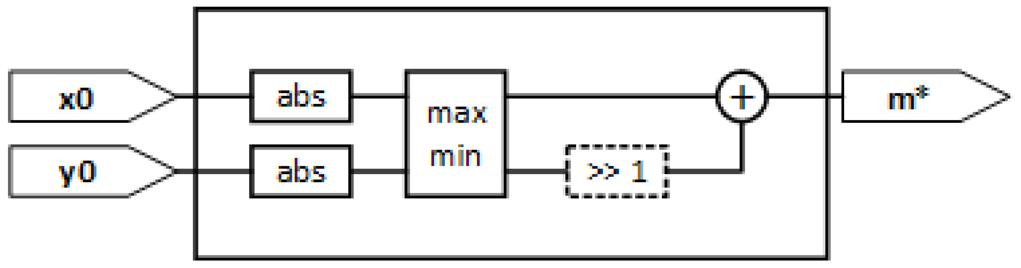
The circuit for a fast magnitude estimation is based on the alphamax-betamin technique [13]. The magnitude estimation is a linear combination of the max and min absolute values of the input coordinates, as shown in Equation (3). The choice of a and b values depends on the metric that the approximation in Equation (3) wants to minimize. If the max absolute error of the entire input space is the selected metric, the optimum numerical values are a ≈ 0.9551 and b ≈ 0.4142. 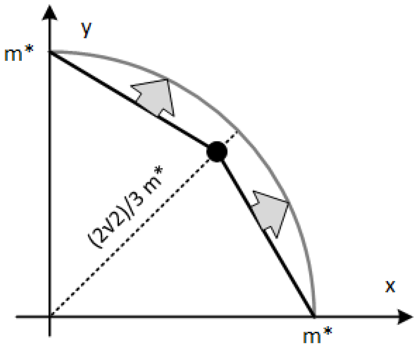A coarse approximation for a simplified and fast implementation can be a = 1 and b = 0.5. This means that only an abs block, a comparison block and a virtual shift plus addition have to be implemented in hardware, while avoiding the use of multipliers. Using the architecture in Figure 1, which implements the calculation in Equation (3), the estimated magnitude m* is always higher than the real one. For example, if the coordinates are equal, i.e., $\left|x_0\right|=\left|y_0\right|$ the result of Equation (3) is $m*=\left|x_0\right|\cdot 3/2$ while the real magnitude is $m_{real}=\left|x_0\right|\cdot \sqrt{2}=m*\cdot 2\sqrt{2}/3$. In the case of $\left|x_0\right|=0then{m}_{real}=m*=\left|y_0\right|$, while if $\left|y_0\right|=0then{m}_{real}=m*=\left|x_0\right|$. 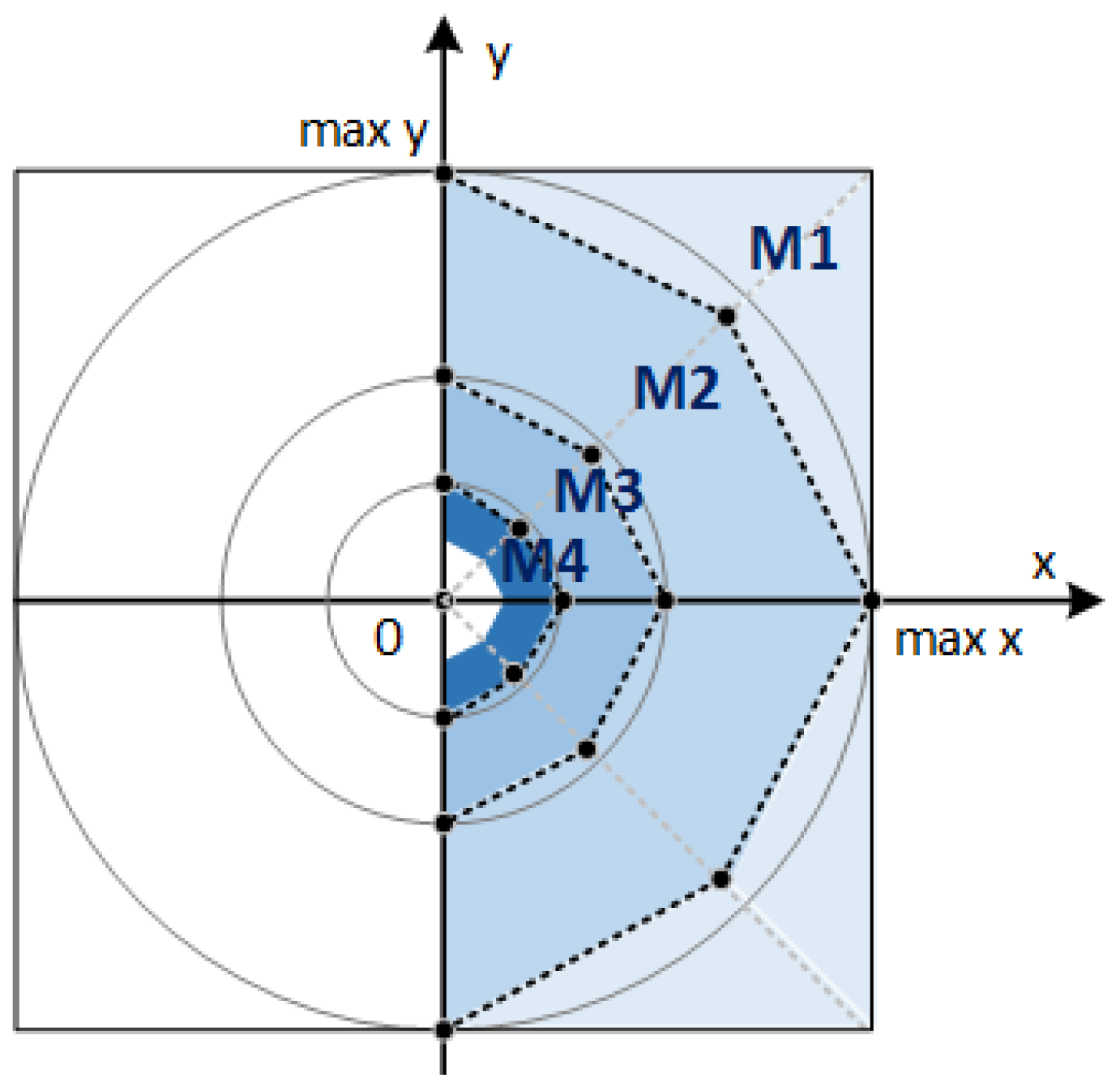These considerations are shown in Figure 2, where the light grey circumference arc includes the possible positions of the points with the estimated magnitude m*. Figure 2 also shows the real position corresponding to the case $\left|x_0\right|=\left|y_0\right|$ with a black point and two segments, drawn with a black line, connecting this point to the points corresponding to the cases of $m_{real}=m*=\left|x_0\right|or\left|y_0\right|$. In Figure 2 the two segments are always under the computed magnitude arc. It should be noted that for all the input points belonging to the two segments, the corresponding magnitude m*, estimated with Equation (3) and the circuit in Figure 1, is the radius of the light grey circumference arc in Figure 2.

$$m*=a\max (\left|x_0\right|,\left|y_0\right|)+b\min (\left|x_0\right|,\left|y_0\right|)$$

(3)

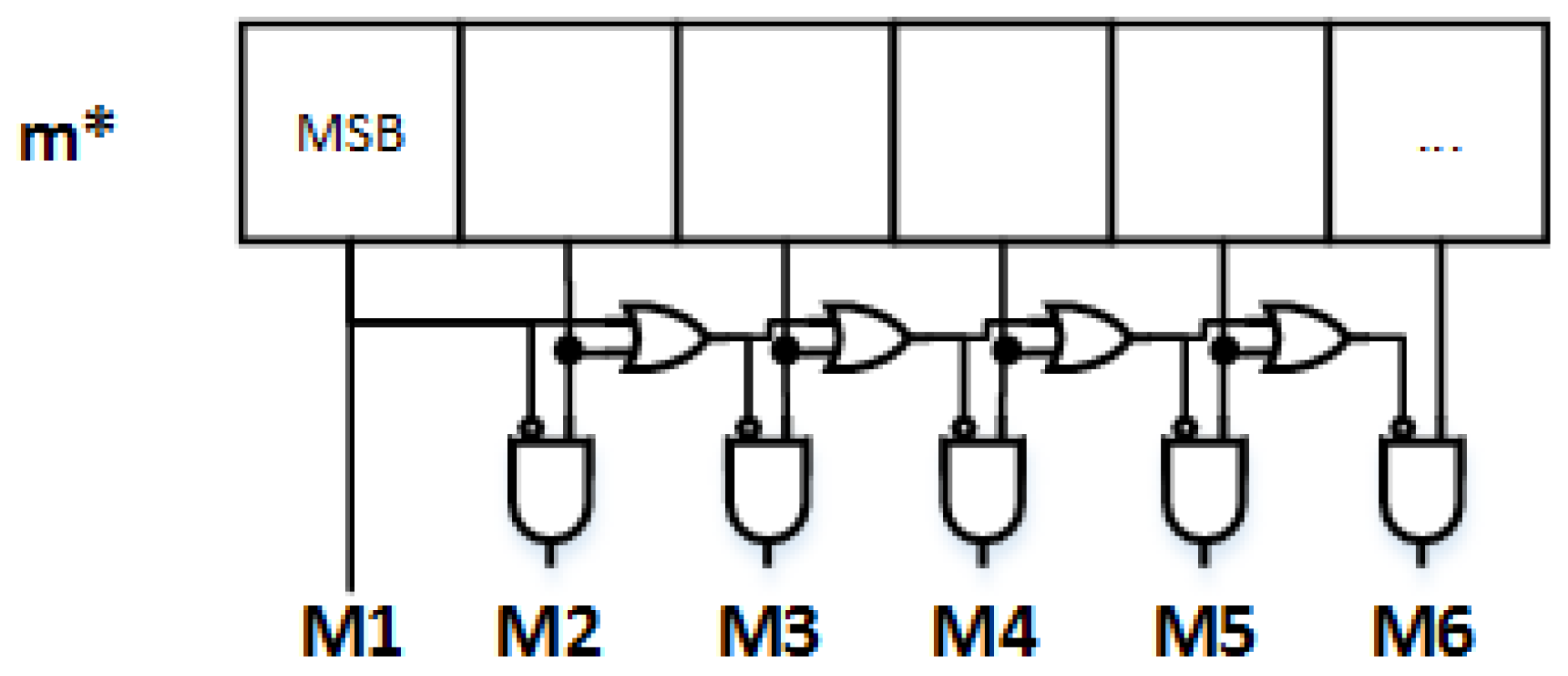
If the x and y data paths are quantized on the M bit signed, the magnitude estimator in Figure 1 needs M bit unsigned to represent m*. The idea is to segment the input space, based on m*. We label as M1 area the set of points with the MSB (Most Significant Bit) of m*, say m*[M-1], equal to one. If a point is not in the M1 area then we look for the m*[M-2] bit to mark it in the M2 area, and so on, until the desired level of segmentation is reached. Figure 3 shows the first area segments of the input coordinates while Figure 4 shows a simple circuit able to extract the logical information of the segmented area as a function of m*.

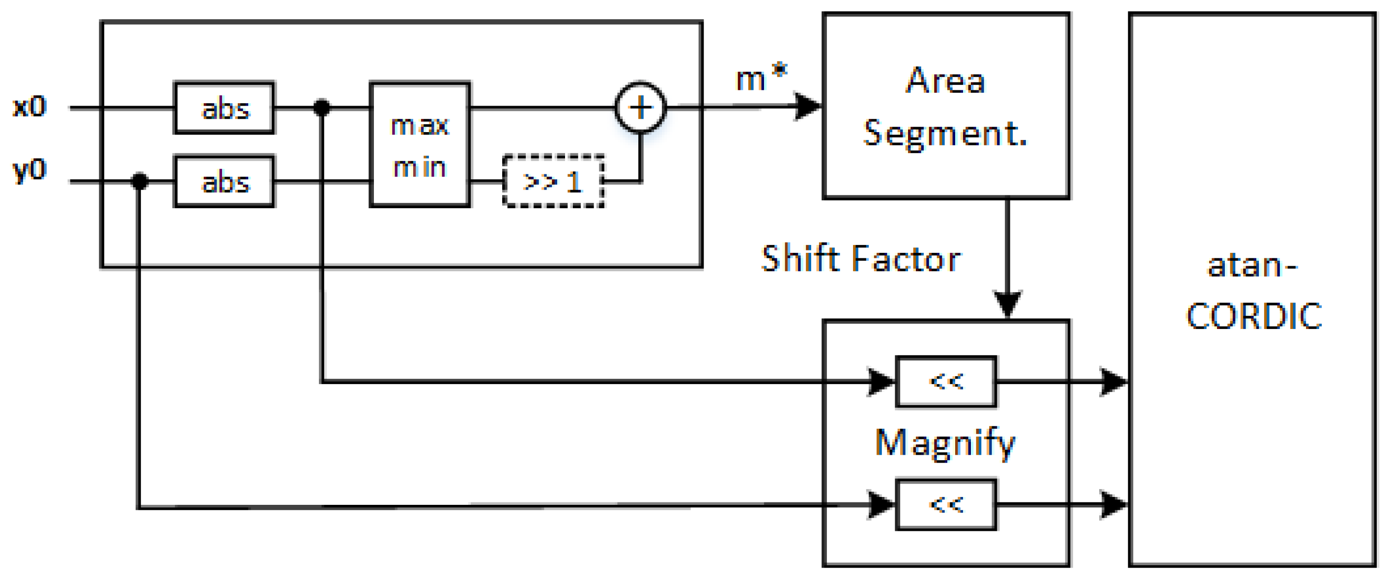
When the Mk area for a point is known, a shift factor (SFk) is selected and applied to the $x_0$ and $y_0$ input coordinates in a way that the magnified coordinates reach the M1 area or the M2 area. In other words, we want to work with points that are always in the first two segments, far from the zero point. Equation (4) shows the doubling rule to correctly shift the inputs starting from the M3 area (SF1 = 0, SF2 = 0). Figure 5 shows the architecture of the improved atan-CORDIC with the fast magnitude estimator and the input magnification. A difference compared to other CORDIC optimizations and CORDIC architectures in the literature [7,8,9,14,15,16] is the maintenance of the standard CORDIC core, to which we add a low-complexity pre-processing unit, working on the input ranges, thus minimizing the overall circuit complexity overhead.

$$x_0{2}^{S{F}_k};y_0{2}^{S{F}_k}:S{F}_k=k-2k\ge 3$$

(4)

3. Computation Accuracy Evaluation

The architecture proposed in Figure 5 has been designed as a parametric HDL macrocell where the bit-width of the x, y and angle data paths can be customized at synthesis time, as well as the number n of CORDIC iterations and the number of input segments in Figure 3. For the atan-CORDIC core, a pipelined fully sequential architecture has been implemented. The choice of these parameters implies different optimization levels. An empirical parameter exploration is mandatory to characterize the sub-optimum architecture depending on the application requirements.

The quantization parameters in the fixed-point implementation are the number of bits of the x and y coordinates, the number of bits of the angle quantization, the number of iterations of the algorithm and the number of segmented areas. Giving the angle resolution in K bits, we know that the useful number of iterations comes from the relation where the quantized angle on the ATR set goes under half of its LSB (Last Significant Bit), being $\mathrm{LSB}=\pi /2^{K-1}$. Overestimating the angle ${\alpha }_i$ with $2^{-i}$, we can compute the useful limit of iterations with

$$2^{-i}<LSB/2\Rightarrow i>K-{\log }_2\pi \approx K-1.65$$

(5)

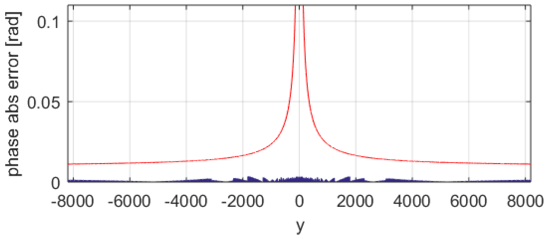
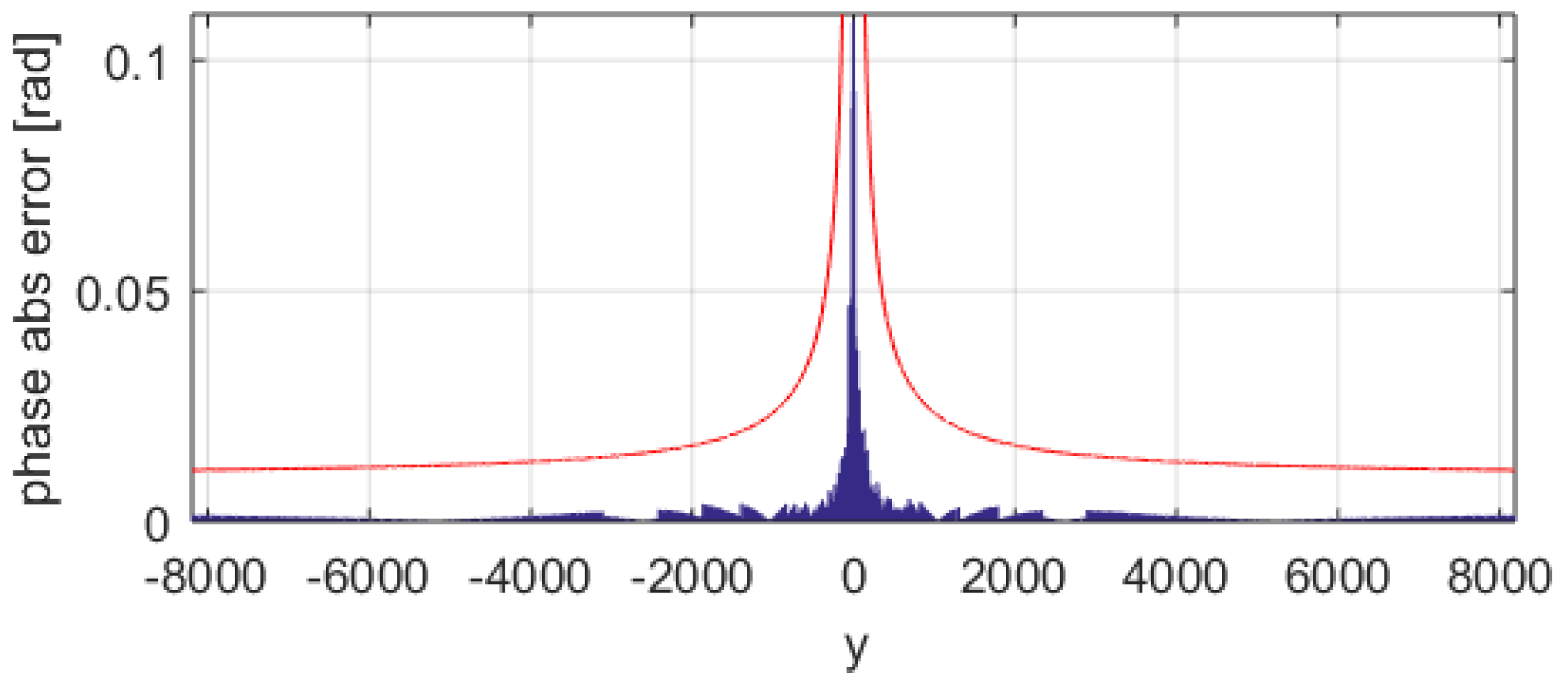
This means that the iteration index goes from 0 to K − 1 (K iterations). As a case study, we present an atan-CORDIC with an x, y data path on 14-bit signed, an angle data path on 12-bit signed and n = 12 iterations (iteration index from 0 to 11). To understand the phase error behavior, a first analysis is done holding the x coordinate (x = 16 in the example) and sweeping the entire y space. Figure 6 shows the absolute error in radians of the computed phase with the standard CORDIC with a blue trace. We see that for points near zero, the phase error increases significantly. The max error is ~0.10865 rad (about 71 LSB). Using the improved atan-CORDIC with nine area segments (max pre-magnification of 128), we get the result in Figure 7. In Figure 7, the blue trace is the absolute error. In Figure 7, the max error is ~0.0035 rad (less than 3 LSB). The same analysis can be extended through the x coordinates, collecting the maximum error of each run. 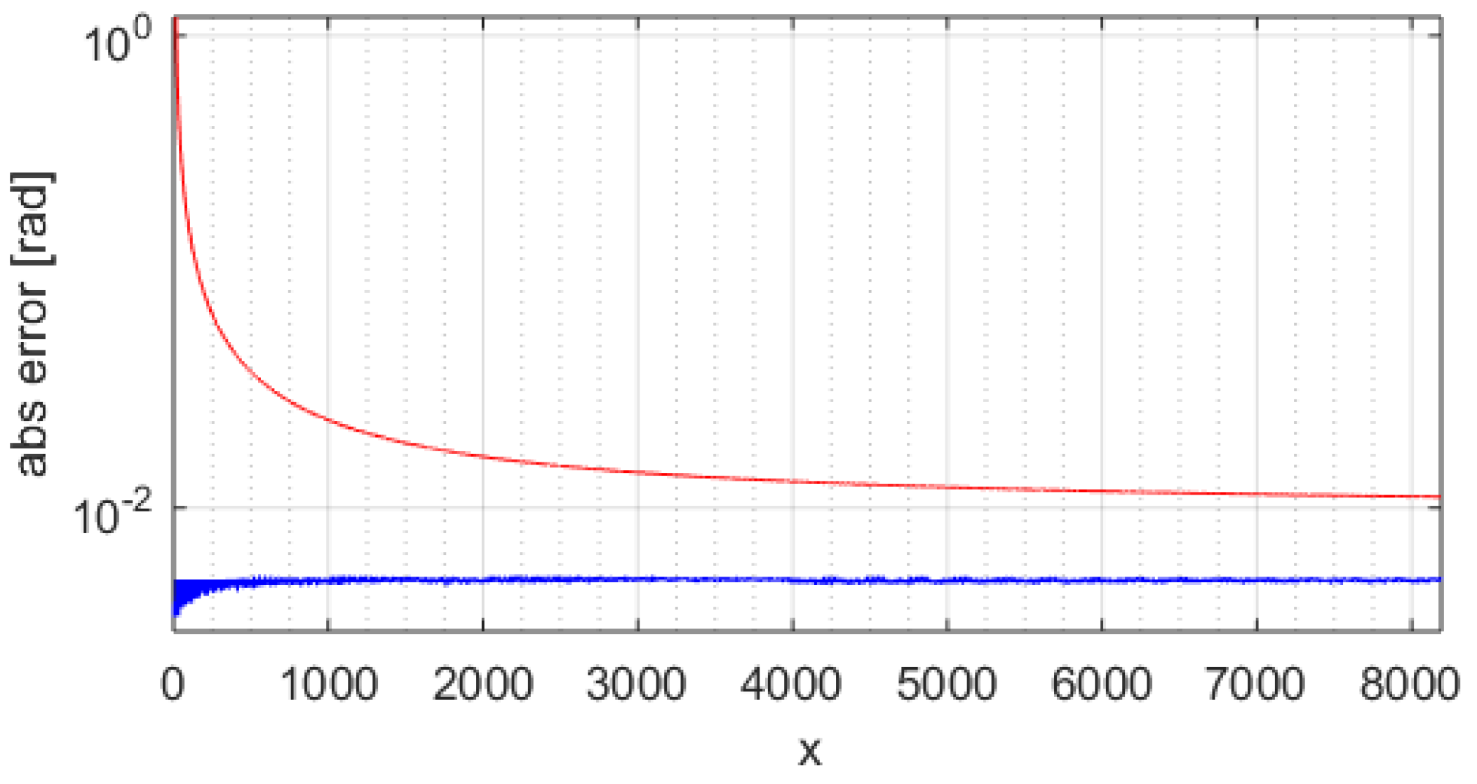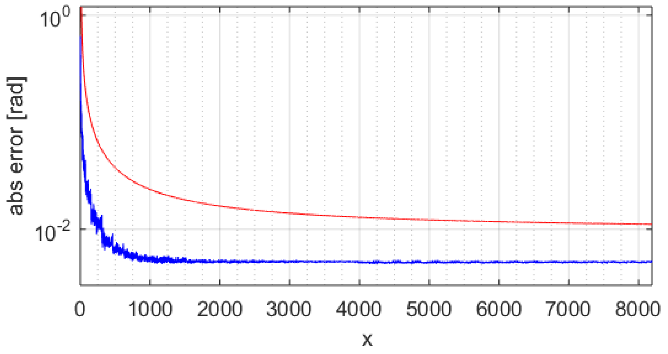Figure 8 shows the standard atan-CORDIC phase errors with a blue trace where the maximum is ~0.6355 rad (about 414 LSB). Figure 9 shows the improved atan-CORDIC errors with a blue trace where the maximum is ~0.0052 rad (less than 4 LSB). The red line in Figure 6, Figure 7, Figure 8 and Figure 9 is the coarse upper-bound error evaluated with Equation (2).

To evaluate further the performance of the proposed architecture, the maximum error on the angle is analyzed by varying some quantization parameters, as reported in

Table 1. Max angle error expressed in LSB of the standard (std) vs. the proposed (our) CORDIC, K = 12, 12 iterations from 0 to 11, bits for x and y from 10 to 14, M areas from 6 to 9.

	M Areas
	6		7		8		9
x, y Bits	std	our	std	our	std	our	std	our
10	414	50	414	16	414	16	414	16
11	414	50	414	13	414	10	414	10
12	414	50	414	13	414	10	414	6
13	414	50	414	13	414	10	414	4
14	414	50	414	13	414	10	414	4

and

Table 2. Max angle error expressed in LSB of the standard (std) vs. the proposed (our) CORDIC, K = 12, nine iterations from 0 to 8, bits for x and y from 10 to 14, M-areas from 6 to 9.

	M areas
	6		7		8		9
x, y Bits	std	our	std	our	std	our	std	our
10	410	45	410	15	410	15	410	15
11	410	45	410	10	410	10	410	10
12	410	45	410	9	410	9	410	8
13	410	45	410	9	410	9	410	7
14	410	45	410	9	410	9	410	7

. In Table 1 the light cells show the standard CORDIC maximum error, fixed to 414 LSB (410 LSB in Table 2), while the grey cells represent the improved CORDIC maximum angle error. From the analysis of Table 1 and Table 2, it is clear that increasing the number of M areas and/or increasing the bit width of the x and y data paths allows reducing the error. Instead, if we compare the peak error as a function of the number of iterations n (12 iterations in Table 1 vs. nine iterations in Table 2), the minimum is obtained for Table 2, which uses a number of iterations lower than the maximum 12 estimated from Equation (5), with K = 12. This can be justified by the fact that, as discussed in Section 1, the quantization in the data paths of the fixed-point implementation causes a truncation error that is accumulated in every loop of the algorithm.

Indeed, in

Table 3. Max angle error expressed in LSB of the standard vs. proposed CORDIC (K = 12, 12 bits for x and y data paths, six M areas).

	Max. Number of Iterations
	2	3	4	5	6	7	8	9	10	11	12
Standard CORDIC	512	302	252	333	374	394	404	409	412	413	414
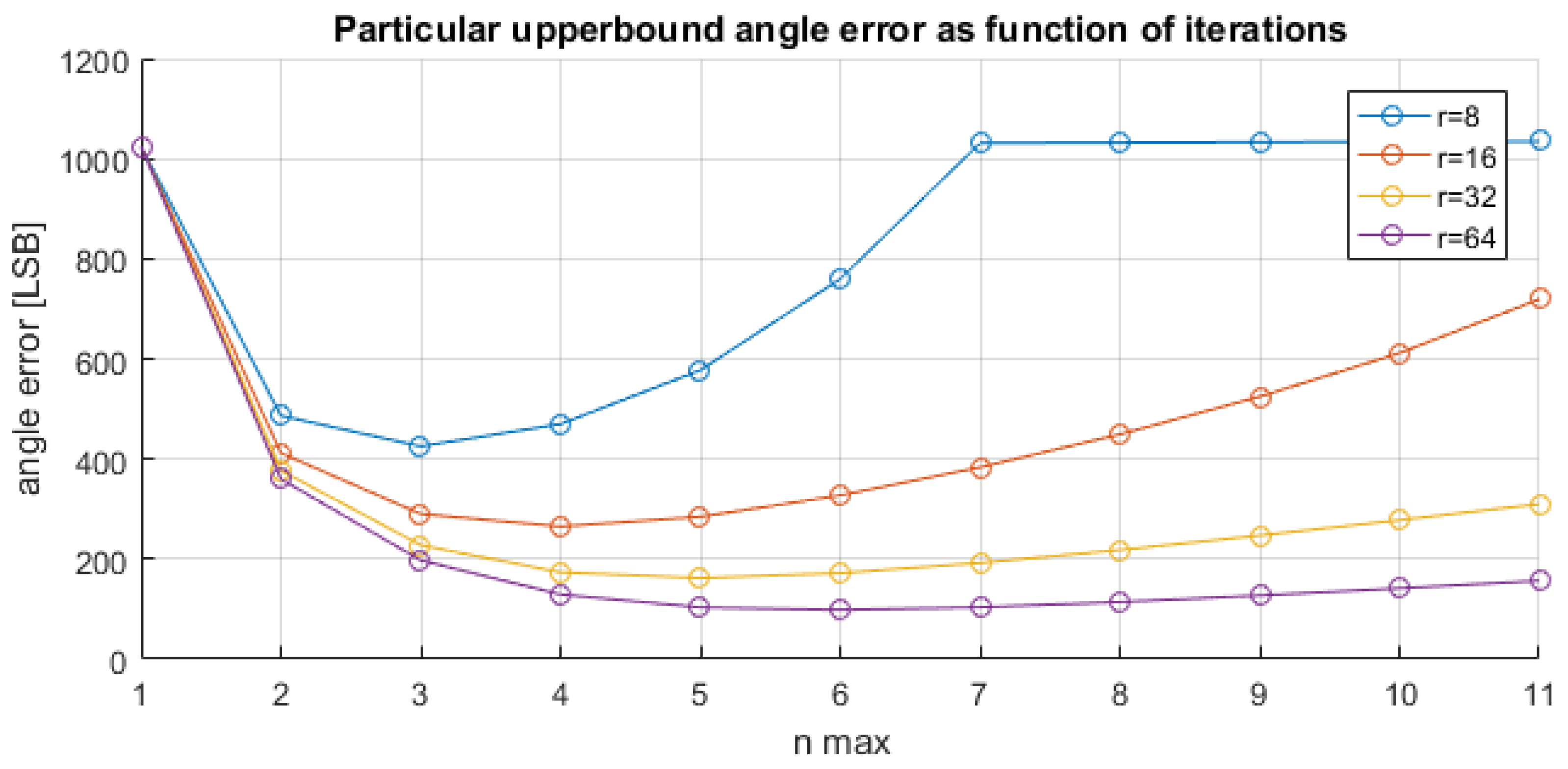
Proposed CORDIC	512	302	160	82	43	30	40	45	48	49	50

we have reported, for both the standard and the proposed CORDIC, the maximum angle error, expressed in LSB, as a function of the number of iterations. For example, the minimum of the maximum angle error is achieved for the proposed CORDIC with seven iterations. This behavior can be theoretically justified, since the maximum angle error is achieved for low magnitude values, i.e., low values of the radius r in Equation (2). Figure 10 plots the error upper bound as a function of the number of iterations, using Equation (2) with $ϵ=1$, $\delta =\pi /2^{K-1}$, $K=12$, and values for the radius $rof8,16,32and64$. In Figure 10, similarly to what is observed in Table 3, there is a first part where the upper-bound error decreases and a second part where the upper-bound error increases.

4. VLSI Implementation and Characterization

The improved CORDIC architecture proposed in Section 2 has been designed in VHDL as a parametric macrocell that can be integrated in any system-on-chip. With reference to the macrocell configuration discussed in Section 3, a synthesis in the standard-cell 180 nm 1.8 V CMOS technology from AMS ag has been carried out. The macrocell design is characterized by a low circuit complexity and low power consumption: about 1700 equivalent logic gates, with a max power consumption (static and dynamic power) of about 0.45 mW when working with a clock frequency of 30 MHz. The overhead due to the innovative parts of this work (fast magnitude estimation and input coordinates magnification) vs. a standard CORDIC implementation in the same technology is limited to 24% in terms of equivalent logic gates and −36% in terms of max working frequency. The processing time of the atan function is n·Tclock, i.e., 0.4 µs when n = 12 with a clock of 30 MHz. As a possible improvement, a pipeline register can be inserted in Figure 5 before the atan-CORDIC core. This way, the complexity increases by about 10%, resulting in 1900 equivalent logic gates, while the working frequency can be increased up to 46 MHz and the power consumption is 0.77 mW. The processing time is (n + 1)·Tclock; with n = 12 iterations of the atan function, the processing time is 0.28 µs.

The comparison of the proposed solution vs. the standard state-of-the-art solution, implemented in the same 180 nm 1.8 V technology, is summarized in

Table 4. Performance of the proposed CORDIC solution vs. standard solution.

IP macrocell	Standard CORDIC	This work	[6]	[8]
Equivalent gates	1400	1700 (1900 pipelined)	8000	18,000 + 32kB RAM + 512 kB E2PROM
Clock frequency, MHz	46	30 (46 pipelined)	10	60
Max. angle error	0.6355 rad	6.1 × 10−3 rad	N/A (K = 16, n = 20)	2.42 × 10−5 rad
Processing latency, µs	0.28	0.4 (0.28 pipelined)	N/A	35
Power consumption, mW	0.57	0.45 (0.77 pipelined)	N/A	24

. Table 4 shows also the comparison with other known CORDIC computation architectures [6,8]. In [8], an embedded solution is proposed using a 32-bit ART7TDMI-S core (18,000 equivalent gates) plus 32 kB of RAM (Random Access Memory) and 512 kB of EEPROM (Electrically Erasable Programmable Read Only Memory). With a clock of 60 MHz, the solution in [8] implements an atan evaluation in 35 µs and an angle error of 2.42 × 10⁻⁵ rad with an optimized algorithm. At 60 MHz with 180 nm 1.8 V CMOS technology, the ARM7-TDMIs has a power consumption of about 24 mW. Although [8] is optimized to achieve a lower error, 2.42 × 10⁻⁵ rad vs. 6.14 × 10³ rad in our implementation, with K = 12, the proposed design outperforms the design in [8] in terms of the reduced processing time, by a factor ×124, the reduced power consumption, by a factor ×31, and the reduced circuit complexity, by a factor ×9.5 . To achieve a similar calculation accuracy as in [8], our IP has been re-synthetized with K = 20. In such a case, the processing time is still within 1 µs and the complexity in the logic gates is still below 4 kgates.

The 180 nm technology node and the target clock frequency have been selected following the constraints of automotive applications where, to face a harsh operating environment (over-voltage, over-current, temperature up to 150 °C), a 180 nm 1.8 V technology ensures higher robustness vs. scaled sub-100 nm CMOS technologies operating with a voltage supply of 1 V. The considered 180 nm technology is automotive-qualified and has a logic gate density of 118 kgates/mm² [18]. The N-MOS supplied at 1.8 V has a voltage threshold of 0.35 mV and a current capability of 600 µA/µm². The P-MOS supplied at 1.8 V has a voltage threshold of 0.42 mV and a current capability of 260 µA/µm².

The proposed improved CORDIC IP has been integrated in an application-specific processor, called SENSASIP [5], to improve the digital signal processing capability of a 32-bit CORTEX-M0 core. Particularly, the SENSASIP chip is used to implement the algorithms in [3,19,20,21] in real time for the sensor signal processing of a 3D Hall sensor and of an inductive position sensor in X-by-wire automotive applications. In these specific applications, the real-time application requirements were met already with a clock frequency for SENSASIP of 8 MHz. Hence, with a 46 MHz clock frequency, the improved CORDIC architecture is about six times faster than required. At 8 MHz, the power consumption of the proposed CORDIC architecture is below 0.1 mW.

It should be noted that the CORDIC computation can be done via software on the 32-bit Cortex core, as is done in [15] for the same class of magnetic sensor position signal conditioning. However, as proved in [5], the use of the proposed CORDIC macrocell integrated on-chip allows for savings in power consumption up to 75%. It should be noted that the proposed macrocell can be also integrated in FPGA technology, as in [16], in case the application of interest requires an FPGA implementation rather than a system-on-chip one.

5. Conclusions

In this work, we propose an improved architecture for arctangent computation using the CORDIC algorithm. A fast magnitude estimator works with a pre-processing magnification to rescale the input coordinates to an optimum range as a function of the estimated magnitude. After the scaling, the inputs are processed by the standard CORDIC algorithm implemented without changing any data path precision. The improved architecture is generic and can be applied to any atan-CORDIC implementation. The architecture improvement is achieved with a low-circuit complexity since it does not require any special operation, but only comparison, shift and add operations. Several case studies have been analyzed, considering a resolution for x and y from 10 to 14 bits, a resolution of 12 bits for the angle, a number of iterations from two to 12, and from six to nine area segments. The bit-true analysis shows that the maximum absolute error in the atan-CORDIC computation improves by at least two orders of magnitude, e.g., in Table 1 from 414 LSB to 4 LSB. The proposed macrocell has been integrated in a system-on-chip, called SENSASIP, for automotive sensor signal processing. When implemented in an automotive-qualified 180 nm 1.8 V CMOS technology, two configurations are available. The first one has a circuit complexity of 1700 logic gates, a max clock frequency of 30 MHz, a CORDIC processing time of 0.4 µs and a power consumption of 0.45 mW. The second configuration has an extra pipeline stage, and has a circuit complexity of 1900 logic gates, a max clock frequency of 46 MHz, a CORDIC processing time of 0.28 µs and a power consumption of 0.77 mW. These values are compared well to state-of-the-art works in the same 180 nm technology node. The 46 MHz clock value is six times higher than what is required (8 MHz) by real-time automotive sensor signal conditioning applications. In these operating conditions, the power consumption of the proposed solution is below 0.1 mW.