On the Generality of Codebook Approach for Sensor-Based Human Activity Recognition


1
Pattern Recognition Group, University of Siegen, Hoelderlinstr. 3, D-57076 Siegen, Germany
2
Department of Knowledge Engineering, University of Economics in Katowice, Bogucicka 3 Str., 40-226 Katowice, Poland
*
Author to whom correspondence should be addressed.
Electronics 2017, 6(2), 44; https://doi.org/10.3390/electronics6020044
Submission received: 29 April 2017
/
Revised: 23 May 2017
/
Accepted: 26 May 2017
/
Published: 1 June 2017
(This article belongs to the Special Issue Data Processing and Wearable Systems for Effective Human Monitoring)
Abstract
:With the recent spread of mobile devices equipped with different sensors, it is possible to continuously recognise and monitor activities in daily life. This sensor-based human activity recognition is formulated as sequence classification to categorise sequences of sensor values into appropriate activity classes. One crucial problem is how to model features that can precisely represent characteristics of each sequence and lead to accurate recognition. It is laborious and/or difficult to hand-craft such features based on prior knowledge and manual investigation about sensor data. To overcome this, we focus on a feature learning approach that extracts useful features from a large amount of data. In particular, we adopt a simple but effective one, called codebook approach, which groups numerous subsequences collected from sequences into clusters. Each cluster centre is called a codeword and represents a statistically distinctive subsequence. Then, a sequence is encoded as a feature expressing the distribution of codewords. The extensive experiments on different recognition tasks for physical, mental and eye-based activities validate the effectiveness, generality and usability of the codebook approach.
1. Introduction
Recently, mobile devices equipped with different sensors have been made low-power, low-cost, high-capacity and miniaturised [1,2,3]. This allows continuous recording of sensor data related to the daily life of a person [4,5]. Especially, in addition to traditional accelerometers, gyroscopes and GPSs, state-of-the-art sensors can capture physiological signals such as blood volume pressure, heart rate, galvanic skin conductance, respiration rate and electrooculogram (EOG) [6,7,8,9,10]. This offers a possibility to recognise not only physical behaviours of the person, but also his/her mental states (i.e., emotions) and health conditions. Thus, activities in this paper include all of these ”high-level” descriptions that can be potentially extracted from ”low-level” sensor data. This sensor-based human activity recognition is useful for various applications, like intelligent human-computer interaction, effective lifelogging and healthcare (ambient-assisted living).
Since data obtained from a sensor are usually formed of a sequence representing the value (or vector of values) at each time point, sensor-based human activity recognition can be formulated as sequence classification. This is generally solved in a machine learning framework, where a classifier (recognition model) is built that takes a sequence as input and predicts its activity class. First, ”training sequences” that are already annotated with activity classes are analysed. This leads to construct a classifier that captures characteristics of sequences in each activity class. Then, it is used to categorise ”test sequences” for which activity classes are unknown [1,3].
One of the most important issues is the choice of sequence representation. As the raw representation of a sequence includes irrelevant information to classification, a classifier should be built on a more abstracted representation, called ”feature”, which expresses relevant characteristics of the sequence. A good feature makes it easier to categorise the sequence into the appropriate activity class. Regarding this, many existing methods rely on ”hand-crafted” features that are designed based on prior knowledge and manual investigation. Examples of hand-crafted features are the mean and variance of values in a sequence, the mean of first-order derivatives, and power spectrum in a certain frequency domain [1,3,11,12,13,14,15,16,17]. However, hand-crafted features have two crucial problems: The first is the lack of statistical validity. For example, rather than the mean value of a sequence, the “mean plus 1.5” may lead to more accurate recognition. The second problem is the difficulty of representing the detailed information in a sequence. In other words, a person can only perceive coarse-grained tendencies of sequences.
To overcome these problems, this paper focuses on feature learning which extracts useful features from a large amount of data [18,19]. In particular, a simple but effective one called codebook approach is adopted. This has been originally developed in the fields of object detection/recognition and image/video classification [20,21]. The original codebook approach analyses a large number of patches (small regions) in images and constructs a codebook consisting of characteristic patches called codewords. An image is then represented by a feature signifying the distribution of codewords. Here, codewords are extracted as cluster centres obtained by grouping numerous patches into clusters of visually similar ones. Thus, each codeword indicates a statistically distinctive patch. In addition, the feature of an image preserves the detailed information by extracting hundreds/thousands of codewords. We apply this codebook approach to sequence classification by regarding patches in images as subsequences collected by sliding a window over sequences. Consequently, a codebook consists of abundant codewords representing statistically distinctive subsequences, and details of a sequence are encoded by a feature expressing their distribution.
This paper aims to evaluate the generality of the codebook approach in various activity recognition tasks by considering the availability of unobtrusive wearable/mobile sensors. Specifically, the following three tasks are selected: The first is the recognition of mental activities (i.e., emotions like “joy”, “anger” and “hate”) using physiological data, such as blood volume pressures, galvanic skin conductances and respiration rates [11]. These can be measured by latest wristbands [6,7] and clip-type sensor [8]. The second task is the recognition of physical activities (e.g., jumping, bending, sitting down and standing up) using accelerometer data of different body parts [22]. For example, body, hand and head movements can be measured using accelerometers installed in a smartphone, wristband [6,7] and intelligent glasses [9], respectively. The last task is the recognition of eye-based activities (e.g., reading, writing and watching TV) using EOG data [10], which characterise eye movements and can be captured by state-of-the-art intelligent glasses [9]. Through these experiments, we justify the generality of the codebook approach for recognising various activities in daily life settings.
2. Related Work
Recent survey papers on sensor-based human activity recognition [1,3] present that the mean and variance (standard deviation) of values in a sequence are the most popular features. However, only with these, too much information is lost. To compensate this, researchers use additional features like the mean of first-order derivatives, zero-crossing rate, power spectrum obtained by Fast Fourier Transform (FFT), entropy of spectral powers, and biomedically engineered features (e.g., average duration between heart beats, inhalation/exhalation duration, and eye-blinking rate) [10,11,12,13,14,15,16,17]. As extreme examples, the methods in [12,13,14] use more than 100 features. Although the usage of many features is one option to preserve details of a sequence, hand-crafting each of them requires both prior knowledge and laborious manual investigation. Also, several methods adopt the “point-to-point comparison” where values in a sequence are matched with those in another sequence [23,24]. In other words, these methods do not extract features, but directly use raw values in sequences. However, it is reported that the point-to-point comparison is brittle to noise, and features capturing high-level structures are necessary for accurate sequence classification [25,26].
Some sensor-based human activity recognition methods employ the codebook approach by making different modifications [22,27,28,29,30] (Codebook-based methods have also been developed in the fields of sequence/time series classification [25,26,31,32]. However, these are not discussed in this paper, in order to focus on sensor-based human activity recognition.). These methods mainly differ in how to represent a subsequence for codebook construction. Note that subsequences need to be represented with features so that they can be compared and grouped into clusters. For clear discussion, a feature of a subsequence is termed as a local “feature”, while the term “feature” is used for a sequence and derived by collecting local features of subsequences. In [28], targeting accelerometer and gyroscope sequences, codewords are extracted by representing subsequences with local features that indicate physical parameters of human motion, such as movement intensities, motion magnitudes along the vertical/heading direction, and the correlation of accelerations between the gravity and heading directions. In [29], for ElectroEncephaloGram (EEG) and ElectroCardioGraphic (ECG) sequences, local features of subsequences are extracted as approximation coefficients obtained by Discrete Wavelet Transform (DWT). The method in [30] analyses sequences of blood pressures and simply uses the mean value of a subsequence as its local feature. The methods in [22,27] address multi-dimensional sequences obtained from several accelerometer sensors, and represent a subsequence with a local feature expressing means and variances in individual dimensions.
Compared to the above existing methods, our method extracts no local feature and groups subsequences into clusters by comparing their raw values. In other words, the vector of raw values in a subsequence is used as its local feature. Hence, our method does not rely on problem-specific local features like the ones in [28,29]. Moreover, in contrast to very rough local features (means and variances) [22,27,30], the detailed information of a subsequence is maintained by its raw values. Although one may think that raw values are sensitive to noise, a huge number of subsequences are available. This allows us to robustly discover statistically distinctive subsequences as codewords. This is demonstrated in Section 4 that shows codewords extracted using raw values. Like this, compared to the existing methods, our codebook-based method is the most basic and general. To our best knowledge, in the field of sensor-based human activity recognition, there is little work that benchmarks method performances on the same dataset. One reason may be that researchers prefer to creating a new system where a developed method is tested on their own dataset. Actually, all the methods described above are tested on different datasets. In contrast, by keeping the most basic and general form of the codebook approach, we aim to examine its generality in different recognition tasks. Also, some generic extensions (soft assignment and early fusion) for the codebook approach are studied.
Finally, one of the most popular feature learning approaches is “deep learning” that extracts a feature hierarchy with higher-level features formed by the composition of lower-level ones based on a multilayer neural network [18]. Deep learning has been recently applied to sensor-based human activity recognition [33,34]. However, it is very difficult and requires extensive trial-and-error to appropriately choose a network architecture and many hyper-parameters (e.g., learning rate, momentum, weight decay and sparsity regularisation) [19,35]. In contrast, our method only involves four hyper-parameters (i.e., the window size and sliding size for subsequence collection, the number of codewords and the smoothing parameter). Despite this simplicity, the experimental results in Section 4 show that stable and reasonable performances are accomplished in different recognition tasks. Furthermore, characteristic subsequences are extracted as codewords by only tuning a few hyper-parameters. Therefore, our codebook-based method is considered to be an easy-to-use analytical tool for various sensor data.
3. Codebook-Based Human Activity Recognition
Figure 1 shows an overview of our codebook-based method, where emotion recognition on sequences of respiration rates is used as an example task. Our method consists of the following three steps: Firstly, the codebook construction step in Figure 1a collects subsequences from sequences and groups them into clusters of similar ones. A codebook is constructed as a set of codewords each of which is the centre of a cluster. Secondly, at the codeword assignment step in Figure 1b, the feature of a sequence is extracted by assigning each subsequence to the most similar codeword. In other words, this feature is a histogram representing the frequency of each codeword. Last, the classifier training/test step in Figure 1c is based on the fact that sequences represented by such features can be considered as points in a multi-dimensional space. A classifier is trained so as to discriminate between training sequences annotated with a certain activity class and those annotated with the others. In Figure 1c, such a classifier is depicted by the dashed line representing the boundary between the mental activity “anger” and the others. Based on this boundary, the classifier determines the activity class of a test sequence.
3.1. Codebook Construction
Let us assume a window of size w. From each sequence, subsequences are collected by locating the window at every l time points. Then, k-means clustering [36] is performed to find N clusters consisting of similar subsequences. It should be noted that each subsequence represents values at w time points, so it can be considered as a w-dimensional vector. Based on this, the similarity between two subsequences is measured as their Euclidean distance. In addition, to focus on shapes of subsequences, a translation is applied to each subsequence so that the value at the first time point is zero. Lastly, since k-means clustering depends on initial cluster centres that are randomly determined, it is conducted 10 times to select the best result yielding the minimum sum of Euclidean distances between subsequences and their assigned cluster centres. Based on the best clustering result, a codebook consisting of N codewords is obtained.
3.2. Codeword Assignment
For each sequence, a histogram-type feature representing the distribution of N codewords is extracted. First, subsequences are collected in the same way to codebook construction. Then, for each subsequence, the most similar codeword is found and its frequency is incremented. Finally, the probabilistic feature representation is obtained by normalising the frequency of each codeword so that the sum of frequencies of all the N codewords is one.
The approach described above deterministically assigns a subsequence to a single codeword. This hard assignment lacks the flexibility to deal with the uncertainty in codeword assignment. For example, in Figure 1b, the first subsequence is the most similar to the second codeword from the left, but it is also similar to the rightmost one. Hence, it is not reasonable to only increment the frequency of the former codeword. To handle the uncertainty, soft assignment is adopted to implement smooth assignment of a subsequence to multiple codewords based on kernel density estimation [37]. Let and be the sth subsequence () in a sequence and the nth codeword (), respectively. The smoothed frequency of is computed as follows:
Here, is the Euclidean distance between and , and is its Gaussian kernel value where is a smoothing parameter. A large causes a strong smoothness so that smoothed frequencies of all codewords become similar. Note that when is similar to (i.e., is small), is large, so offers a large contribution to (this contribution is normalised by the sum of kernel values for all codewords, as shown in the denominator of Equation (1)). This way, soft assignment yields a feature representing the smoothed distribution of codewords based on their similarities to subseuqneces. Finally, to avoid numerical underflow, Equation (1) is calculated by firstly computing with the log-sum-exp trick [38].
3.3. Classifier Training/Test
Let us build a binary classifier that distinguishes training sequences labelled with a target activity from the other training sequences. The former and latter are called “positive sequences” and “negative sequences”, respectively. To gain the high discrimination power, a variety of characteristic subsequences need to be considered using hundreds of codewords (i.e., N is large). That is, each sequence is represented with a high-dimensional feature. Hence, a Support Vector Machine (SVM) is used because of its effectiveness for high-dimensional data [39]. The SVM draws a classification boundary based on the margin maximization principle so that the boundary is placed in the middle between positive and negative sequences. This makes the generalisation error of the SVM independent of the number of dimensions [39]. Actually, the combination of the codebook approach and an SVM has been justified in many image/video classification tasks using features with thousands of dimensions [21,40]. For a test sequence, the trained SVM outputs a scoring value between 0 and 1 based on its distance to the classification boundary [41]. A larger value indicates that the test sequence is more likely to belong to the target activity class. Finally, the recognition of C activities is conducted using C SVMs, each of which is built as a binary classifier for one activity. Then, the activity of a test sequence is determined as the one characterised by the highest SVM value.
The following two points deserve attention: The first is the “imbalanced problem” that in general negative sequences significantly outnumber positive ones, since a huge variety of sequences can be negative [42]. This may have an adverse influence on classifier training, because meaningless hypotheses that classify almost all sequences as negative get high accuracies on training sequences. However, it has been experimentally proven that SVMs are not affected by the imbalanced problem [43]. In particular, SVMs are appropriately trained even in a situation where the number of negative sequences is over 200 times the number of positive ones. The second point is the setting of SVM parameters. Considering the generality, our method uses the Radial Basis Function (RBF) kernel that has one parameter to control the complexity of a classification boundary. This parameter is set to the mean of squared Euclidean distances among training sequences, because it stably offers reasonable performances without conducting computationally expensive cross validation [44,45]. In addition, the SVM parameter to control the penalty of mis-classification is empirically set to 2. This SVM parameter setting is used throughout all the experiments.
3.4. Fusion of Multiple Features
Different sensors produce multiple sequences for the same activity instance. The fusion of features extracted from these sequences is essential for accurate activity recognition. Let us assume that every activity instance is associated with M features, each of which is a histogram-type feature based on a separately constructed codebook. In general, there are two fusion approaches, early fusion and late fusion [46]. The former concatenates M features into a high-dimensional feature. For example, if all of M features are N-dimensional, early fusion creates an -dimensional feature. Late fusion firstly builds M classifiers that are individually built on single features. Then, outputs by these classifiers are fused into a final scoring value.
We adopt early fusion for the following reasons: The first is its simplicity and computational efficiency, because SVM training/test can be performed on concatenated features with no modification. In particular, each of M features is normalised so that the sum of frequencies of all codewords is one (this is true also for soft assignment). Hence, M features are fairly treated in the high-dimensional feature created by their simple concatenation. On the other hand, late fusion requires not only training/test of M classifiers, but also training/test of a classifier for fusing outputs by those M classifiers. The second reason is that early fusion can consider correlations among dimensions in different features, while late fusion based only on classifier outputs cannot consider them.
4. Experimental Results
This section presents the experimental results of our codebook-based method on three sensor-based human activity recognition tasks. For each task, a brief description of the dataset is firstly provided. Some implementation details are then explained to tune our method and its parameters. Afterwards, the results are discussed from different perspectives like hard/soft assignment, fusion of multiple sensors, and comparison to existing methods. In particular, for fair performance comparison, our method is run in the same evaluation setting as existing methods. Finally, the computational cost of our method is discussed.
It should be noted that, except the translation to make the first value of a subsequence zero (see the “codebook construction” part in Section 3) and the statement in the “implementation details” part in each task, no other processing like noise filtering has been done. With respect to this, our codebook-based method has a robustness to noise because the feature of a sequence is extracted by abstracting raw subsequences into statistically distinctive codewords. Even if these subsequences are noisy, as long as they can be assigned to codewords having similar overall value changes, our method can appropriately extract the feature of the sequence.
4.1. Mental Activity Recognition Using Physiological Data
4.1.1. Dataset Description
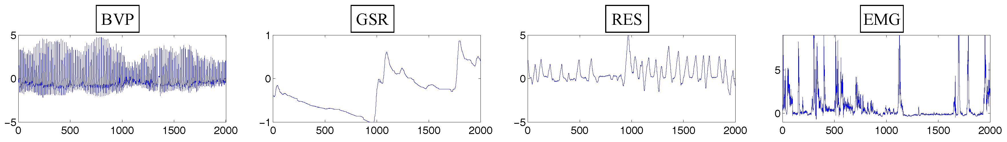
The dataset introduced in [11] is used to examine the effectiveness of our method on mental activity (emotion) recognition using physiological sensor data. The dataset includes four types of physiological sequences, Blood Volume Pressure (BVP), Galvanic Skin Response (GSR), RESpiration (RES) and ElectroMyoGram (EMG). These sequences are collected for eight emotions (“no-emotion”, “anger”, “hate”, “grief”, “platonic-love”, “romantic-love”, “joy” and “reverence”) of one subject for 20 days. For each type, there are 160 sequences () that consist of values at 2001 time points sampled at 20 Hz. Figure 2 presents the BVP, GSR, RES and EMG sequences when the subject felt “anger” at the first day.
4.1.2. Implementation Details
To reduce the bias of values depending on days, for each type, eight sequences for one day are normalised so as to have the mean zero and the variance one. We have not conducted any other processing like noise filtering. A codebook is constructed using subsequences collected from 160 sequences for each type. The performance is evaluated in the same way as [11]. Specifically, leave-one-out cross validation is conducted where 159 sequences are used for training and the remaining one is used for test. This is iterated until all the sequences are tested. The emotion recognition performance is measured as the accuracy (percentage) of how many sequences are correctly classified.
Our method has three main parameters, the window size w and the sliding size l for subsequence collection, and the number of codewords N. First, l is the parameter to control how densely subsequences are sampled from a sequence. In image/video classification, it is widely accepted that denser sampling leads to a better performance [45,47]. Thus, l is set to 8 so that more than 230 subsequences are sampled from a sequence. We consider that these subsequences are enough for estimating the distribution of codewords in the sequence. Regarding w and N, to avoid under-/over-estimating recognition accuracies, we test all the 20 combinations defined by and (It is possible to test parameters at a finer granularity level and find a better parameter combination. However, we aim to validate the generality and usability of the codebook approach, by showing that it can produce reasonable performances with roughly defined parameters.). In addition, to capture periodic characteristics of RES sequences, their spectra called “RES_sp” are analysed. Specifically, subsequences obtained by and are represented with amplitude spectra via FFT (the transform length is 256 and the hanning window is used). Then, using , these subsequences are clustered to construct a codebook in terms of amplitude spectra. Therefore, in this experiment, one emotion instance is represented by five features BVP, GSR, RES, EMG and RES_sp, which are integrated using early fusion.
4.1.3. Results
For each feature, a distribution of recognition accuracies is obtained by collecting the accuracy for every combination of w and N. An example is shown in Figure 3a that presents the accuracy distribution acquired using RES and hard assignment. Since grasping an overall trend from this distribution is difficult, it is summarised into a box plot as depicted in Figure 3b. This indicates the maximum, upper quartile, median, lower quartile and minimum of the accuracy distribution. In Figure 3b, the leftmost box plot for each feature represents the accuracy distribution obtained by hard assignment. Except RES_sp, the remaining five plots indicates the accuracy distributions resulting from soft assignment with . For RES_sp, are used as in Figure 3b. Moreover, the rightmost group of box plots represents the accuracy distributions produced by early fusion of five features. Note that these distributions are computed using the 12 combinations of and , because of the difference between the w range for RES_sp and the one for the other features (i.e., w and N are the same for all features). As indicated by the transition of median accuracies for each feature in Figure 3b, soft assignment yields more accurate recognition than hard assignment, although accuracies depend on . In addition, box plots for early fusion are located at considerably higher positions than the ones for single features. This validates the effectiveness of early fusion.
We check more detailed characteristics of early fusion. Through the experiment in Figure 3, we found that high recognition accuracies are stably accomplished using and (our preliminary experiment showed that larger and cause the performance degradation). In addition, based on Figure 3b, leading to the maximum median accuracy is chosen for each feature. Specifically, and 4 are used for BVP, GSR, RES, EMG and RES_sp, respectively. Under this setting, all possible combinations of five features are tested. Figure 4 shows the transition of accuracies by these combinations, where each accuracy at the upper part is obtained using the black-coloured features in the “fusion indicator” at the lower part. For example, the sixth accuracy from the left () is acquired using BVP and GSR features, as depicted by their black-coloured elements in the fusion indicator. Figure 4 indicates that higher accuracies are generally attained using more features. In particular, compared to the accuracy using all features, only two feature combinations yield higher accuracies, by RES, EMG and RES_sp, and by GSR, RES, EMG and RES_sp. Here, the difference among these three accuracies is very small, and selecting a specific subset of features lacks the generality. It can be said that a nearly optimal performance is achieved using early fusion, which simply concatenates all the features into a single high-dimensional feature. In other words, the discrimination between relevant and irrelevant features is appropriately done by a classifier (i.e., SVM), so it does not have to be done manually in advance.
Apart from early fusion, Figure 4 implies one issue regarding a domain for codebook construction. In Figure 4, the codebook for RES is constructed by clustering subsequences in the time domain, while the one for RES_sp is based on the frequency domain. Here, the accuracy () only by RES and the one () only by RES_sp are very similar. In addition, the accuracy by the fusion of RES and RES_sp is , which indicates no improvement compared to only using RES. This can be interpreted that RES and RES_sp features describe similar characteristics, so their fusion does not yield any improvement. In other word, the codebook constructed in the time domain covers aspects represented by the codebook in the frequency domain, because frequency aspects emerge as shapes of subsequences. Thus, it can be thought as enough to only consider the time domain for codebook construction. This is also checked by the comparison between the accuracy by BVP, GSR, RES and EMG to the accuracy by the fusion of all features. The addition of frequency-based RES_sp only leads to a very small improvement.
Table 1 shows the comparison between the accuracy of our method developed in this study and that of the method in [11]. For each of BVP, GSR, RES and EMG sequences, the latter extracts a six-dimensional statistical feature representing the mean, standard deviation, mean of first-order derivatives etc. Based on early fusion of such features, each emotion instance is represented by a 24-dimensional feature. Then, feature dimension selection and probabilistic classifier training/test are conducted. The right column in Table 1 shows the accuracies that are reported in [11] (for fair comparison, we omit accuracies based on heuristics like physiology-dependent and day-dependent features, and accuracies on reduced sets of emotions). Since our main objective is to examine the usefulness of features extracted by the codebook approach, the accuracies in parentheses in Table 1 are obtained in the settings where only features are different. Specifically, our method extracts 2048-dimensional features by early fusion of four -dimensional features on BVP, GSR, EMG and RES (see the corresponding entry in Figure 4), while the comparison method uses 24-dimensional features described above. Except this, both methods use the same SVM training/test. The resulting accuracies signify that our method significantly outperforms the comparison method. This validates the effectiveness of features extracted by the codebook approach.
Finally, let us examine what kind of codewords are extracted by our method. For each feature, Figure 5 visualises 15 codewords that are extracted by grouping 37,600 subsequences collected by and into clusters. Rectangular regions display codewords (subsequences) representing values at 128 time points, except RES_sp for which the first 50 of 128 spectral amplitudes are displayed for clear visualisation. The number under a rectangular region indicates the ID of the corresponding codeword. For example, the top-left rectangular region in BVP presents the 461th codeword. As can be seen from Figure 5, our method could successfully extract codewords as subsequences exhibiting various characteristic value changes. In addition, one can further investigate codewords to discover knowledge about their relations to activities. For example, codewords specific to certain activities can be found by checking the entropy of a codeword over activities. In Figure 5, the 461th codeword for BVP appears 26 times over the whole set of sequences, but 25 appearances occur in sequences for “no-emotion” (). Moreover, 27 of 31 appearances of the 74th codeword for RES occur in sequences for “grief” (). This way, our codebook-based method offers an easy-to-use analytical tool where a user only has to tune three parameters w, l and N.
4.2. Physical Activity Recognition Using Accelerometer Data
4.2.1. Dataset Description
The dataset established in [22] is used to examine the effectiveness of our method on physical activity recognition using accelerometer data. In addition to these data, the dataset includes motion capture (mocap) data, multi-view video data by stereo vision, RGB-D data by Kinect cameras, and audio data recorded by microphones. However, considering the data acquisition capability by wearable/mobile devices, only accelerometer data are used in this experiment. These data are captured using six three-axis wireless accelerometers attached to left/right wrists, left/right hips and left/right ankles. Figure 6 displays example sequences obtained from these six accelerometers, each of which produces a three-dimensional sequence at the sampling rate of about 30 Hz. Sequences are recorded for the following 11 activities performed by 12 subjects: 1. jumping in place; 2. jumping jacks; 3. bending (hands up all the way down); 4. punching (boxing); 5. waving (two hands); 6. waving (right hand); 7. clapping hands; 8. throwing a ball; 9. sit down then stand up; 10. sit down; and 11. stand up. Every subject performs each action five times. Thus, there are a total of 660 activity executions, each of which is associated with a set of six three-dimensional sequences. Actually, two executions failed to be recorded, so this experiment is carried out on 658 executions.
4.2.2. Implementation Details
First of all, since accelerometer data are acquired in a controlled setting, no normalisation has been done on sequences. In other words, raw accelerometer data are used without any preprocessing like noise filtering. For each of six accelerometers, our method constructs one codebook where codewords represent characteristic “three-dimensional subsequences”. In other words, these codewords capture correlations among three dimensions. To this end, a subsequence collected by a window of size w is represented as a -dimensional vector, where the first w, the subsequent w and the last w dimensions represent values in the first, second and third dimensions, respectively. Except this, no modification is needed for codebook construction (the translation to make the first value zero is separately executed for each dimension). At the codeword assignment step, subsequences in a three-dimensional sequence are assigned to codewords by computing similarities in terms of their -dimensional vector representations. Six features extracted from three-dimensional sequences for all accelerometers can be integrated by early fusion.
We follow the evaluation setting in [22] where sequences for the first seven subjects are used for training, and sequences for the remaining five subjects are used for testing. Codebooks are constructed only using training sequences. The performance of a method is evaluated with an accuracy (classification rate) representing the percentage of correctly classified sequences. The parameters w, l and N are set as follows: First, l is set to 2 by considering that sequences in this dataset relatively short, because they are collected with a low sampling frequency of 30 Hz. In other words, small l is needed to collect many subsequences from a short sequence, so that the resulting feature appropriately represents the distribution of codewords. The 15 combinations defined by and are tested, and accuracies obtained by them are summarised into a box plot. Note that a few sequences are too short and their lengths are less than w, so no subsequence can be collected. Such sequences are represented by the feature where all dimensions have zero. Finally, early fusion is used to concatenate six features each of which is computed using the same w, l, N and .
4.2.3. Results
Figure 7 shows box plots of accuracies obtained by single features and their fusion. For each feature (or fusion), the leftmost box plot is acquired with hard assignment, while the remaining six plots are obtained using soft assignment with , respectively. First of all, as can be seen from the leftmost box plot for the fusion, an accuracy of is achieved even with hard assignment. Because of this very high accuracy, the effectiveness of soft assignment is not so clear. Nonetheless, by taking a close look at box plots for the fusion, median accuracies are slightly improved. Actually, while hard assignment achieves the accuracy of only by one parameter combination , the same accuracy is obtained by four parameter combinations , , and at . This implies that soft assignment appropriately treats the uncertainty in codeword assignment, so that high accuracies are stably obtained in many parameter settings. Compared to the fusion, the degree of uncertainty in each single feature is lower. This can be considered as one reason for the weak effect of soft assignment on single features. In addition, the accuracy obtained by hard assignment on a single feature may be nearly maximum, so no further improvement can be achieved only with this feature.
Finally, the accuracy of presented above is significantly better than that of reported in [22]. Indeed, the method in [22] uses the codebook approach. The following three issues can be considered as reasons for the big performance difference: The first is that the method in [22] extracts codewords only by considering variances in individual dimensions of a subsequence. In consequence, codewords only represent very brief information of subsequences. The second issue is the small number of subsequences (30) collected from each sequence. This seems insufficient not only for performing statistically robust clustering of subsequences to extract codewords, but also for extracting a feature that appropriately represents the distribution of codewords in a sequence. The last issue is the small number of codewords (20), so the discrimination power of a resulting 20-dimensional feature is not so high. Regarding these three issues, our method compares raw values in subsequences so as to extract codewords representing detailed characteristics. In addition, subsequences are sampled from a sequence much more densely using , and a much larger number of codewords () are used.
4.3. Eye-Based Activity Recognition Using EOG Data
4.3.1. Dataset Description
Our method is tested on eye-based activity recognition using the EOG dataset created in [10]. The eye acts as an electric potential field where the cornea and retina work as the positive and negative poles, respectively. EOG signals represent changes in this electric potential field. Two signal components, horizontal EOG (hEOG) and vertical EOG (vEOG), are used to capture two-dimensional eye movements. Examples of hEOG and vEOG sequences are shown in Figure 8. It has recently become possible to easily collect such EOG sequences using a wearable device like intelligent glasses [9]. In [10], EOG sequences are collected to recognise activities related to eye movements. At the sampling rate 128 Hz, hEOG and vEOG sequences are recorded for the following six activities: 1. copying a text; 2. reading a printed paper; 3. taking handwritten notes; 4. watching a video; 5. browsing the Web; and 6. pause (no specific activity). Each of eight subjects did two executions of six activities in random orders. That is, the dataset consists of 16 hEOG/vEOG sequences. Note that these are not divided into segments corresponding to activities, instead every time point is labelled with one of six activities (A part of time points are annotated with two “noise” labels (distraction speak and distraction phone). These time points are excluded from the performance evaluation.). Hence, different from the previous experiments where already-segmented sequences are categorised into activities, this experiment aims to label each time point in an unsegmented sequence with the appropriate activity, by considering values around this time point.
4.3.2. Implementation Details
First, each of 16 hEOG (or vEOG) sequences is normalised to have the mean zero and the variance one. No other preprocessing like noise filtering has been done. For one activity execution by a subject, the set of hEOG and vEOG sequences is regarded as a two-dimensional sequence. Similar to the previous experiment, a codebook is constructed by clustering “two-dimensional subsequences”, where the first w and the remaining w dimensions represent values in the hEOG and vEOG sequences, respectively. Based on this, codebook construction is conducted using about 186,000 subsequences collected from two-dimensional sequences for all the activity executions. Early fusion is not needed in this experiment.
Apart from subsequences for codebook construction and codeword assignment, another type of subsequences are extracted from a two-dimensional sequence by sliding a window of 30 s (3840 time points) with the sliding size s (32 time points). Such a subsequence is represented by a feature and classified into one of six activities. The activity of a time point is determined by considering classification results of subsequences around it. For clear discussion, this kind of subsequence to be classified is called a “c-subsequence”. In other words, the c-subsequence is encoded into a feature by assigning fine subsequences in it to codewords. Note that the comparison method in [10] uses the same c-subsequence described above. We aim to compare the method in [10] to ours in the same setting.
The performance evaluation is conducted in the same “leave-one-person-out scheme” as [10]. Two-dimensional sequences for all but one subject are used for training, and two-dimensional sequences for the excluded subject are used for test. Under this setting, let us consider SVM training for a certain activity. Our method does not use c-subsequences containing time points annotated with different activities, but only uses c-subsequences in each of which all time points are labelled with the same activity. As a result, about 10,000 positive c-subsequences and about 50,000 negative c-subsequences are available for training an SVM. Considering the computational cost, we use all the positive c-subsequences, and randomly select negative c-subsequences so that the total number of training c-subsequences is 30,000 (our preliminary experiment showed that using more negative c-subsequences does not yield performance improvement). Then, the SVM is applied to about 10,000 c-subsequences in test sequences. The method developed in [45] is used to efficiently conduct large-scale SVM training/test.
The overall score of each time point is computed using the “max-pooling” approach. This associates the time point with the SVM score, which is the maximum among the scores obtained for c-subsequences covering this time point. This way, for each activity, an SVM is trained and applied to test sequences. Thereby, every time point is associated with overall scores for all the six activities. Finally, each time point is classified into the activity with the highest overall score. By comparing such predicted activities to the ground truth, the performance in terms of a subject is measured as the average of time-point-wise precisions and the one of recalls over six activities.
Regarding the parameter setting, l is firstly set to 16 so as to collect more than 200 subsequences from a c-subsequence. Then, w is set to 128 by testing . Afterwards, N is configured as 4096 among . Finally, is used after testing .
4.3.3. Results
Table 2 shows the performance comparison between our method and the method in [10]. Each column indicates a subject-specific performance, except the last one that represents the average of subject-specific performances over eight subjects. The left and right numbers in each element represent the average of time-point-wise precisions and that of recalls over six activities, respectively, when sequences for the corresponding subject are tested. The comparison between the second and third rows in Table 2 verifies the effectiveness of soft assignment. The bottom row shows the performance of the method in [10]. It is about higher than the performance of our method using soft assignment. However, the method in [10] heavily relies on heuristics and prior knowledge. For example, preprocessing for baseline drift removal conducts wavelet transformation involving non-intuitive parameters like the decomposition level and order of Daubechies wavelet. Detection of eye movements (saccades, fixations and blinks) requires several carefully-tuned thresholds. Furthermore, 90 features are hand-crafted based on detected eye movements. Moreover, a parameter for temporally smoothing classification results is needed. Compared to this, our method has no problem-specific process and only uses intuitively-tunable parameters. In addition, except the normalisation for zero-mean and unit-variance, no other preprocessing like drift or noise removal has been conducted. Therefore, our codebook-based method is an easy-to-use analytical tool, because it can achieve reasonable performance with no problem-specific knowledge, preprocessing or tuning.
4.4. Discussion about Computational Costs
The experiments below have been done using a single CPU core in Xeon X5690 (3.47 GHz) for codebook construction, and a single core in i7-3970X (3.50 GHz) for codeword assignment and SVM training/test. First, targeting 160 RES sequences in the dataset [11], 37,600 subsequences are collected with and for codebook construction. Ten repetitions of k-means clustering with clusters take about 13 min and 362 MB memory. To extract a 512-dimensional feature from a sequence of length 2001, hard and soft assignments demand and s, respectively. Then, SVM training with 159 training sequences and its test on one test sequence take and s, respectively (about 130 MB memory is used). These times are obtained using the method, which is developed for large-scale SVM training/test and implements batch computation of distances among many sequences using matrix operation [45]. Since this batch computation involves an overhead to transfer features of sequences to the Matlab environment, the test time in the parenthesis is obtained without using the batch computation.
Similarly, from 16 EOG sequences in the dataset [10], 186,386 two-dimensional subsequences are gathered using and . Ten repetitions of their clustering into clusters take about h and GB memory. Then, s (hard assignment) and s (soft assignment) are required to encode a c-subsequence of length 3840 into a 4096-dimensional feature. Using the method in [45], SVM training on 30,000 training c-subsequences takes s and about 25 GB memory, and its test on 7752 c-subsequences needs s and about 735 MB memory (the time for encoding c-subsequences into 4096-dimensional features is excluded). Like this, batch distance computation in [45] is effective for large-scale SVM training/test. Also, without using the batch distance computation, SVM test on one c-subsequence only takes s.
Let us assume that codebook construction and SVM training have been done in advance, and sensor signals are sent to a PC in real-time. For a situation that is similar to the first experiment described above, recognition of one activity using one feature is carried out at about 24 Hz (=1/0.041), since almost all time is spent for feature extraction. In a situation like the second experiment, recognition of one activity is executed at about Hz (=1/0.255). Also, if real-time processing is not necessary, it is possible to run SVM test with batch distance computation in the night when a user is sleeping.
Considering the above-mentioned computational efficiency, we have developed an actual activity recognition system and released its demonstration video on the Web [48]. Roughly speaking, the system recognises 11 physical activities (e.g., lying, sitting, standing, walking, stretching a hand etc.) using seven sensors in a smartphone (accelerometer, gravity, gyroscope, linear accelerometer and magnetometer) and two sensors in a smartwatch (accelerometer and gyroscope). The recognition is performed every s (the actual time required for executing one recognition is only about s). For the first four sensors with the sampling rate 200 Hz, features are extracted using and , while and are used to extract features from the remaining three sensors with the sampling rate 50 or 67 Hz. Each feature is obtained as an -dimensional vector with hard assignment. Early fusion is used to merge features for the seven sensors into a 7168-dimensional vector, and the SVM-based recognition is performed in exactly the same way as described in Section 3. No other processing has been done in the system. As demonstrated in the video, very accurate activity recognition is achieved by our system based on the codebook approach.
5. Conclusions and Discussion
The extensive experiments in this paper have justified the generality of the codebook approach as well as its usability. Specifically, targeting various types of sequences shown in Figure 2, Figure 6 and Figure 8, our codebook-based method achieved high or reasonable performances using a few intuitively tunable parameters, and not-using any specific knowledge or heuristics. In addition, even with this ease of use, our method can be used to extract codewords specific to a certain activity as discussed in the context of Figure 5. This suggests a practical implication for end-users like clinicians. That is, previously unknown, interesting knowledge could be discovered if the above kind of specific codewords extracted from physiological (or accelerometer) sequences would be investigated by a clinician who is familiar with physiology (or kinematics).
The following three issues will be explored in the future: The first is that a simple histogram-type feature in this paper cannot precisely encode the distribution of codewords. Thus, we will adopt features based on more sophisticated distribution models like Gaussian Mixture Model (GMM) [45] and Fisher encoding [40,49]. Especially, these features are represented as very high-dimensional vectors with more than 10,000 dimensions, so that accurate activity recognition can be achieved using a simple and fast classifier like linear SVM. The second issue is the incorporation of hidden variables into a classifier. This has potentials to solve various problems in sensor-based human activity recognition. For example, in the preparation of training sequences, it is difficult or labour-intensive to label the interval of each activity in a sequence. One practical approach is to provide a label that just represents the occurrence of the activity in a sequence. In this case, using a classifier where hidden variables represent intervals, it is possible to jointly conduct the identification of suitable intervals and their classification into activities [50]. Also, sequences significantly vary depending on contexts like user’s movements and sensor displacements. This can be handled using a classifier that utilises hidden variables corresponding to contexts, so that a different discrimination function is used depending on a context [51]. Regarding the last issue, we have justified the effectiveness of our codebook-based method by comparing it to the methods, which are presented in the papers originally introducing the used datasets [10,11,22]. We plan to carry out a further comparison of our method to both traditional methods based on hand-crafted features [1,3] and latest methods based on deep learning [33,34].
Supplementary Materials
A demostration video showing the effectiveness of the developed codebook-based activity recognition method is available online at https://www.youtube.com/watch?v=sIL08IE_QLE&t=94s.
Acknowledgments
Research and development activities leading to this article have been supported by the German Federal Ministry of Education and Research within the project “Cognitive Village: Adaptively Learning Technical Support System for Elderly” (Grant Number: 16SV7223K).
Author Contributions
Kimiaki Shirahama played the main role in developing the method, conducting the experiments and writing the paper. Marcin Grzegorzek initiated and leaded the overall research activity.
Conflicts of Interest
The authors declare no conflict of interest. The founding sponsors had no role in the design of the study; in the collection, analyses, or interpretation of data; in the writing of the manuscript, and in the decision to publish the results.
Abbreviations
The following abbreviations are used in this manuscript:
| SVM | Support Vector Machine |
| BVP | Blood Volume Pressure |
| GSR | Galvanic Skin Response |
| RES | RESpiration |
| EMG | ElectroMyoGram |
| EOG | ElectroOculoGram |
| hEOG | horizontal EOG |
| vEOG | vertical EOG |
References
- Bulling, A.; Blanke, U.; Schiele, B. A Tutorial on Human Activity Recognition Using Body-worn Inertial Sensors. ACM Comput. Surv. 2014, 46, 33:1–33:33. [Google Scholar] [CrossRef]
- Chen, L.; Hoey, J.; Nugent, C.D.; Cook, D.J.; Yu, Z. Sensor-Based Activity Recognition. IEEE Trans. Syst. Man Cybern. Part C (Appl. Rev.) 2012, 42, 790–808. [Google Scholar] [CrossRef]
- Lara, D.; Labrador, A. A Survey on Human Activity Recognition using Wearable Sensors. IEEE Commun. Surv. Tutor. 2013, 15, 1192–1209. [Google Scholar] [CrossRef]
- López-Nava, H.; Muñoz-Meléndez, A. Wearable Inertial Sensors for Human Motion Analysis: A Review. IEEE Sens. J. 2016, 16, 7821–7834. [Google Scholar]
- Iosa, M.; Picerno, P.; Paolucci, S.; Morone, G. Wearable inertial sensors for human movement analysis. Expert Rev. Med. Devices 2016, 13, 641–659. [Google Scholar] [CrossRef] [PubMed]
- Garbarino, M.; Lai, M.; Bender, D.; Picard, R.W.; Tognetti, S. Empatica E3—A Wearable Wireless Multi-sensor Device for Real-time Computerized Biofeedback and Data Acquisition. In Proceedings of the 2014 EAI 4th International Conference on Wireless Mobile Communication and Healthcare (Mobihealth), Athens, Greece, 3–5 November 2014; pp. 39–42. [Google Scholar]
- Microsoft Corporation. Microsoft Band|Official Site. Available online: www.microsoft.com/microsoft-band (accessed on 29 April 2017).
- Spire, Inc. Spire–Mindfulness & Activity Tracker. Available online: www.spire.io (accessed on 29 April 2017).
- Ishimaru, S.; Kunze, K.; Tanaka, K.; Uema, Y.; Kise, K.; Inami, M. Smart Eyewear for Interaction and Activity Recognition. In Proceedings of the CHI EA 2015—33rd Annual CHI Conference on Human Factors in Computing Systems, Seoul, Korea, 18–23 April 2015; pp. 307–310. [Google Scholar]
- Bulling, A.; Ward, A.; Gellersen, H.; Tröster, G. Eye Movement Analysis for Activity Recognition Using Electrooculography. IEEE Trans. Pattern Anal. Mach. Intell. 2011, 33, 741–753. [Google Scholar] [CrossRef] [PubMed]
- Picard, W.; Vyzas, E.; Healey, J. Toward Machine Emotional Intelligence: Analysis of Affective Physiological State. IEEE Trans. Pattern Anal. Mach. Intell. 2001, 23, 1175–1191. [Google Scholar] [CrossRef]
- Koelstra, S.; Mühl, C.; Soleymani, M.; Lee, S.; Yazdani, A.; Ebrahimi, T.; Pun, T.; Nijholt, A.; Patras, I. DEAP: A Database for Emotion Analysis Using Physiological Signals. IEEE Trans. Affect. Comput. 2012, 3, 18–31. [Google Scholar] [CrossRef]
- Kim, J.; Andre, E. Emotion Recognition Based on Physiological Changes in Music Listening. IEEE Trans. Pattern Anal. Mach. Intell. 2008, 30, 2067–2083. [Google Scholar] [PubMed]
- Soleymani, M.; Lichtenauer, J.; Pun, T.; Pantic, M. A Multimodal Database for Affect Recognition and Implicit Tagging. IEEE Trans. Affect. Comput. 2012, 3, 42–55. [Google Scholar] [CrossRef]
- Hong, J.H.; Ramos, J.; Dey, A.K. Understanding Physiological Responses to Stressors During Physical Activity. In Proceedings of the 2012 ACM Conference on Ubiquitous Computing, Pittsburgh, PA, USA, 5–8 September 2012; pp. 270–279. [Google Scholar]
- Plarre, K.; Raji, A.; Hossain, S.; Ali, A.; Nakajima, M.; Al’absi, M.; Ertin, E.; Kamarck, T.; kumar, S.; Scott, M.; et al. Continuous Inference of Psychological Stress from Sensory Measurements Collected in the Natural Environment. In Proceedings of the 10th International Conference on Information Processing in Sensor Networks (IPSN), Chicago, IL, USA, 12–14 April 2011; pp. 97–108. [Google Scholar]
- Gu, T.; Wang, L.; Wu, Z.; Tao, X.; Lu, J. A Pattern Mining Approach to Sensor-Based Human Activity Recognition. IEEE Trans. Knowl. Data Eng. 2011, 23, 1359–1372. [Google Scholar] [CrossRef]
- Bengio, Y.; Courville, A.; Vincent, P. Representation Learning: A Review and New Perspectives. IEEE Trans. Pattern Anal. Mach. Intell. 2013, 35, 1798–1828. [Google Scholar] [CrossRef] [PubMed]
- Coates, A.; Lee, H.; Ng, A.Y. An Analysis of Single-Layer Networks in Unsupervised Feature Learning. In Proceedings of the 14th International Conference on Artificial Intelligence and Statistics, Fort Lauderdale, FL, USA, 11–13 April 2011; pp. 215–223. [Google Scholar]
- Csurka, G.; Bray, C.; Dance, C.; Fan, L. Visual Categorization with Bags of Keypoints. In Proceedings of the ECCV International Workshop on Statistical Learning in Computer Vision, Prague, Czech Republic, 11–14 May 2004; pp. 1–22. [Google Scholar]
- Jiang, Y.G.; Yang, J.; Ngo, C.W.; Hauptmann, A.G. Representations of Keypoint-Based Semantic Concept Detection: A Comprehensive Study. IEEE Trans. Multimedia 2010, 12, 42–53. [Google Scholar] [CrossRef]
- Ofli, F.; Chaudhry, R.; Kurillo, G.; Vidal, R.; Bajcsy, R. Berkeley MHAD: A Comprehensive Multimodal Human Action Database. In Proceedings of the IEEE Workshop on Applications of Computer Vision (WACV), Tampa, FL, USA, 15–17 January 2013; pp. 53–60. [Google Scholar]
- Liu, J.; Zhong, L.; Wickramasuriya, J.; Vasudevan, V. uWave: Accelerometer-based Personalized Gesture Recognition and Its Applications. Pervasive Mob. Comput. 2009, 5, 657–675. [Google Scholar] [CrossRef]
- McGlynn, D.; Madden, M.G. An Ensemble Dynamic Time Warping Classifier with Application to Activity Recognition. In Research and Development in Intelligent Systems XXVII; Bramer, M., Petridis, M., Hopgood, A., Eds.; Springer Science & Business Media: Berlin, Germany, 2011; pp. 339–352. [Google Scholar]
- Lin, J.; Li, Y. Finding Structural Similarity in Time Series Data Using Bag-of-Patterns Representation. In Proceedings of the 21st International Conference on Scientific and Statistical Database Management, New Orleans, LA, USA, 2–4 June 2009; pp. 461–477. [Google Scholar]
- Baydogan, M.G.; Runger, G.; Tuv, E. A Bag-of-Features Framework to Classify Time Series. IEEE Trans. Pattern Anal. Mach. Intell. 2013, 35, 2796–2802. [Google Scholar] [CrossRef] [PubMed]
- Huỳnh, T.; Blanke, U.; Schiele, B. Scalable Recognition of Daily Activities with Wearable Sensors. In Proceedings of the 3rd international conference on Location-and context-awareness, Oberpfaffenhofen, Germany, 20–21 September 2007; pp. 50–67. [Google Scholar]
- Zhang, M.; Sawchuk, A. Motion Primitive-based Human Activity Recognition Using a Bag-of-features Approach. In Proceedings of the 2nd ACM SIGHIT International Health Informatics Symposium, Miami, FL, USA, 28–30 January 2012; pp. 631–640. [Google Scholar]
- Wang, J.; Liu, P.; She, M.F.H.; Nahavandi, S.; Kouzani, A. Bag-of-words Representation for Biomedical Time Series Classification. Biomed. Signal Process. Control 2013, 8, 634–644. [Google Scholar] [CrossRef]
- Ordóñez, P.; Armstrong, T.; Oates, T.; Fackle, J. Using Modified Multivariate Bag-of-words Models to Classify Physiological Data. In Proceedings of the IEEE 11th International Conference on Data Mining Workshops (ICDMW), Vancouver, BC, Canada, 11 December 2011; pp. 534–539. [Google Scholar]
- Lin, J.; Khade, R.; Li, Y. Rotation-invariant Similarity in Time Series Using Bag-of-patterns Representation. IJIIS 2012, 39, 287–315. [Google Scholar] [CrossRef]
- Zakaria, J.; Mueen, A.; Keogh, E. Clustering Time Series Using Unsupervised-Shapelets. In Proceedings of the IEEE 12th International Conference on Data Mining, Brussels, Belgium, 10–13 December 2012; pp. 785–794. [Google Scholar]
- Martinez, H.P.; Bengio, Y.; Yannakakis, G.N. Learning Deep Physiological Models of Affect. IEEE Comput. 2013, 8, 20–33. [Google Scholar] [CrossRef]
- Yang, J.B.; Nguyen, M.N.; San, P.P.; Li, X.L.; Krishnaswamy, S. Deep Convolutional Neural Networks on Multichannel Time Series for Human Activity Recognition. In Proceedings of the 24th International Conference on Artificial Intelligence, Buenos Aires, Argentina, 25–31 July 2015; pp. 3995–4001. [Google Scholar]
- Bengio, Y. Practical Recommendations for Gradient-Based Training of Deep Architectures. In Neural Networks: Tricks of the Trade, 2nd ed.; Montavon, G., Orr, G.B., Müller, K.R., Eds.; Springer: Berlin, Germany, 2012; pp. 437–478. [Google Scholar]
- Han, J.; Kamber, M.; Pei, J. Data Mining: Concepts and Techniques, 3rd ed.; Morgan Kaufmann: Burlington, MA, USA, 2011. [Google Scholar]
- Van Gemert, J.C.; Veenman, C.J.; Smeulders, A.W.M.; Geusebroek, J.M. Visual Word Ambiguity. IEEE Trans. Pattern Anal. Mach. Intell. 2010, 32, 1271–1283. [Google Scholar] [CrossRef] [PubMed]
- Murphy, K.P. Machine Learning: A Probabilistic Perspective; The MIT Press: London, UK, 2012. [Google Scholar]
- Vapnik, V.N. Statistical Learning Theory; Wiley-Interscience: New York, NY, USA, 1998. [Google Scholar]
- Chatfield, K.; Lempitsky, V.; Vedaldi, A.; Zisserman, A. The Devil is in the Details: An Evaluation of Recent Feature Encoding Methods. In Proceedings of the British Machine Vision Conference, Dundee, UK, 29 August–2 September 2011; pp. 76.1–76.12. [Google Scholar]
- Chang, C.C.; Lin, C.J. LIBSVM: A Library for Support Vector Machines. ACM TIST 2011, 2, 27:1–27:27. [Google Scholar] [CrossRef]
- He, H.; Garcia, E.A. Learning from Imbalanced Data. IEEE Trans. Know. Data Eng. 2009, 21, 1263–1284. [Google Scholar]
- Shirahama, K.; Matsuoka, Y.; Uehara, K. Hybrid Negative Example Selection Using Visual and Conceptual Features. Multimed. Tools and Appl. 2014, 71, 967–989. [Google Scholar] [CrossRef]
- Zhang, J.; Marszalek, M.; Lazebnik, S.; Schmid, C. Local Features and Kernels for Classification of Texture and Object Categories: A Comprehensive Study. IJCV 2007, 73, 213–238. [Google Scholar] [CrossRef]
- Shirahama, K.; Uehara, K. Kobe University and Muroran Institute of Technology at TRECVID 2012 Semantic Indexing Task. In Proceedings of the TRECVID, Gaithersburg, MD, USA, 26–28 November 2012; pp. 239–247. [Google Scholar]
- Snoek, C.G.M.; Worring, M.; Smeulders, A.W.M. Early Versus Late Fusion in Semantic Video Analysis. In Proceedings of the 13th annual ACM international conference on Multimedia, Singapore, 6–11 November 2005; pp. 399–402. [Google Scholar]
- Nowak, E.; Jurie, F.; Triggs, B. Sampling Strategies for Bag-of-Features Image Classification. In Proceedings of the 9th European conference on Computer Vision, Graz, Austria, 7–13 May 2006; pp. 490–503. [Google Scholar]
- You Tube. Demonstration Video of Sensor-Based Human Activity Recognition. Available online: https://www.youtube.com/watch?v=sIL08IE_QLE&t=101s (accssed on 10 April 2017).
- Shirahama, K.; Grzegorzek, M. Towards Large-scale Multimedia Retrieval Enriched by Knowledge about Human Interpretation: Retrospective Survey. Multimed. Tools Appl. 2016, 75, 297–331. [Google Scholar] [CrossRef]
- Nguyen, M.H.; Torresani, L.; De la Torre, F.; Rother, C. Weakly Supervised Discriminative Localization and Classification: A Joint Learning Process. In Proceedings of the IEEE 12th International Conference on Computer Vision, Kyoto, Japan, 29 September–2 October 2009; pp. 1925–1932. [Google Scholar]
- Zhou, G.T.; Lan, T.; Vahdat, A.; Mori, G. Latent Maximum Margin Clustering. In Proceedings of the NIPS, Lake Tahoe, NV, USA, 5–10 December 2013; pp. 28–36. [Google Scholar]
Figure 1.
An overview of our codebook-based human activity recognition method. Here, sequences of respiration rates are used to illustrate (a) how to construct a codebook; (b) how to extract the feature of a sequence based on the extracted codebook; and (c) how such features are utilised to train/test a classifier that distinguishes the mental activity “anger” from the others.
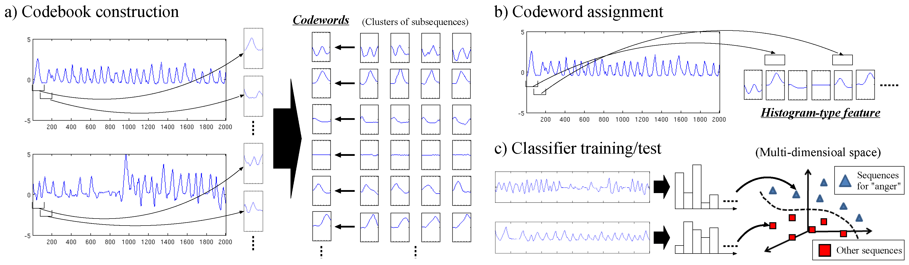
Figure 2.
Examples of four types of physiological sequences in the dataset [11]. From the left, the first, second, third and last sequences represent values of Blood Volume Pressure (BVP), Galvanic Skin Response (GSR), RESpiration (RES) and ElectroMyoGram (EMG), respectively. Note that these sequences are normalised to have the mean zero and the variance one. In addition, to emphasise value changes, each type of sequence is plotted using the vertical axis with a different range.

Figure 3.
(a) An example of an accuracy distribution based on different combinations of w and N; (b) Performance comparison between hard and soft assignments where accuracy distributions are summarised into box plots. Box plots marked as BVP, GSR, RES, EMG, RES_sp and Fusion indicate accuracy distributions obtained for blood volume pressure sequences, galvanic skin response sequences, respiration sequences, electromyogram sequences, respiration spectra, and their fusion, respectively.

Figure 4.
Transition of accuracies depending on fused features. The accuracies at the upper part result from fusing features expressed by the “fusion indicator” at the bottom part. The first, second, third, forth and last rows in the fusion indicator indicate the usages of features extracted from Blood Volume Pressure (BVP) sequences, Galvanic Skin Response (GSR) sequences, RESpiration (RES), ElectroMyoGram (EMG) sequences and RESpiration spectra (RES_sp). If a feature is used, the corresponding element is filled with black, otherwise it is white.

Figure 5.
Examples of codewords extracted by our method. Codewords marked as BVP, GSR, RES, EMG and RES_sp are extracted from Blood Volume Pressure (BVP) sequences, Galvanic Skin Response (GSR) sequences, RESpiration (RES), ElectroMyoGram (EMG) sequences and RESpiration spectra (RES_sp), respectively.
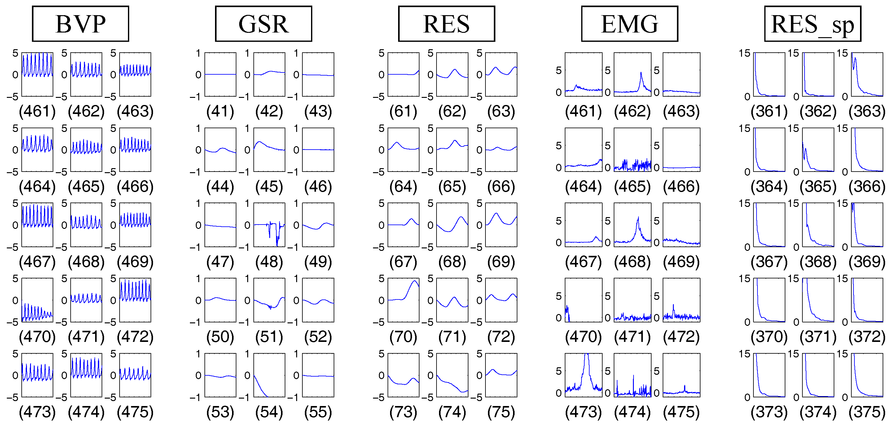
Figure 6.
Examples of three-dimensional sequences from six accelerometers for the activity “jumping in place” in [22].
Figure 6.
Examples of three-dimensional sequences from six accelerometers for the activity “jumping in place” in [22].
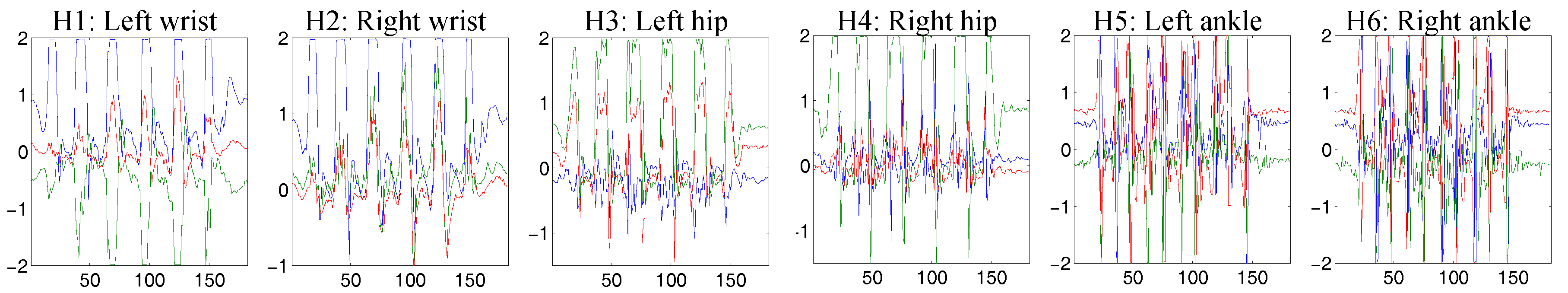
Figure 7.
Accuracies of our method with different s on physical activity recognition using accelerometer sensor data [22].
Figure 7.
Accuracies of our method with different s on physical activity recognition using accelerometer sensor data [22].

Figure 8.
Examples of horizontal and vertical ElectroOculoGram (hEOG and vEOG) sequences in [10].
Figure 8.
Examples of horizontal and vertical ElectroOculoGram (hEOG and vEOG) sequences in [10].


Table 1.
Comparison between our method developed in this study and the one in [11].
Table 1.
Comparison between our method developed in this study and the one in [11].
| This Study | Picard et al. [11] | |
|---|---|---|
| Accuracy | 40.0–46.3% () |
Table 2.
Performance comparison between our method and the one in [10].
Table 2.
Performance comparison between our method and the one in [10].
| Subject 1 | Subject 2 | Subject 3 | Subject 4 | Subject 5 | Subject 6 | Subject 7 | |
| Hard assignment | 51.9/35.2 | 71.9/69.9 | 73.6/55.7 | 32.0/40.8 | 76.4/69.8 | 70.8/56.3 | 75.0/73.0 |
| Soft assignment | 45.6/49.4 | 75.8/74.7 | 79.9/65.5 | 50.9/43.3 | 78.0/70.6 | 75.4/62.4 | 75.5/74.6 |
| Bulling et al. [10] | 76.6/69.4 | 88.3/77.8 | 83.0/72.2 | 46.6/47.9 | 59.5/46.0 | 89.2/86.9 | 93.0/81.9 |
| Subject 8 | Mean | ||||||
| Hard assignment | 53.1/48.4 | 63.1/56.1 | |||||
| Soft assignment | 53.9/50.1 | 66.9/61.3 | |||||
| Bulling et al. [10] | 72.9/81.9 | 76.1/70.5 |
© 2017 by the authors. Licensee MDPI, Basel, Switzerland. This article is an open access article distributed under the terms and conditions of the Creative Commons Attribution (CC BY) license (http://creativecommons.org/licenses/by/4.0/).
Share and Cite
MDPI and ACS Style
Shirahama, K.; Grzegorzek, M. On the Generality of Codebook Approach for Sensor-Based Human Activity Recognition. Electronics 2017, 6, 44. https://doi.org/10.3390/electronics6020044
AMA Style
Shirahama K, Grzegorzek M. On the Generality of Codebook Approach for Sensor-Based Human Activity Recognition. Electronics. 2017; 6(2):44. https://doi.org/10.3390/electronics6020044
Chicago/Turabian StyleShirahama, Kimiaki, and Marcin Grzegorzek. 2017. "On the Generality of Codebook Approach for Sensor-Based Human Activity Recognition" Electronics 6, no. 2: 44. https://doi.org/10.3390/electronics6020044
Note that from the first issue of 2016, this journal uses article numbers instead of page numbers. See further details here.