Accuracy Analysis Comparison of Supervised Classification Methods for Anomaly Detection on Levees Using SAR Imagery


1
School of Computing, University of Southern Mississippi, Hattiesburg, MS 39406, USA
2
Geosystems Research Institute, Mississippi State University, Mississippi State, MS 39759, USA
3
Department of Electrical and Computer Engineering, Mississippi State University, Mississippi State, MS 39762, USA
*
Author to whom correspondence should be addressed.
Electronics 2017, 6(4), 83; https://doi.org/10.3390/electronics6040083
Submission received: 28 August 2017
/
Revised: 7 October 2017
/
Accepted: 12 October 2017
/
Published: 14 October 2017
Abstract
:This paper analyzes the use of a synthetic aperture radar (SAR) imagery to support levee condition assessment by detecting potential slide areas in an efficient and cost-effective manner. Levees are prone to a failure in the form of internal erosion within the earthen structure and landslides (also called slough or slump slides). If not repaired, slough slides may lead to levee failures. In this paper, we compare the accuracy of the supervised classification methods minimum distance (MD) using Euclidean and Mahalanobis distance, support vector machine (SVM), and maximum likelihood (ML), using SAR technology to detect slough slides on earthen levees. In this work, the effectiveness of the algorithms was demonstrated using quad-polarimetric L-band SAR imagery from the NASA Jet Propulsion Laboratory’s (JPL’s) uninhabited aerial vehicle synthetic aperture radar (UAVSAR). The study area is a section of the lower Mississippi River valley in the Southern USA, where earthen flood control levees are maintained by the US Army Corps of Engineers.
1. Introduction
Over the entire US, there are approximately 200,000 km of levee structures of varying designs and conditions. Earthen levees (human-made earthen structures) protect large areas of populated land (hundreds of millions of Americans) and agricultural fields in the United States from flooding (as storm events increase and as river levels rise), as shown in Figure 1.
The catastrophe caused by Hurricane Katrina (August 2005) and the Midwestern United States floods (June 2008) emphasizes the importance of examining levees to improve the condition which makes levees prone to failure during floods. On-site inspection of levees is costly and time-consuming, so there is a need to develop efficient techniques based on remote sensing technologies to identify levees that are more vulnerable to failure under climate change (higher loads) and overloading of water levels (risk, flood loading) [1,2,3]. One type of problem that occurs along these levees which can lead to complete failure during a high-water event are slough slides [1,2,3,4] (also called landslides or slump slides). Slough slides are slope failures along a levee, which leave areas of the levee vulnerable to seepage and failure during high water events. These failures can develop over months to years, and are not quickly noticeable unless they depict some sort of visual identification [5,6,7,8]. Polarimetric synthetic aperture radar (PolSAR) data includes a variety of information which relates to the physical properties of the terrain. Hence, polSAR provides much more information because the transmitted signal is polarized and different polarizations of the backscatter signal are detected [9]. On the other hand, PolSAR appears to have a challenging problem in the classification field due to the complexity of extracting useful information from its multiple polarimetric channels. Nonetheless, investigations with PolSAR imagery have shown that it has great potential for classification and pattern recognition applications [10].
In the past, we have conducted work of detecting anomalies on levees using advanced unsupervised classification methods using polarimetric SAR. In that work, using the parameters entropy (H), anisotropy (A), alpha (α), and eigenvalues (λ, λ1, λ2, and λ3), we implemented several unsupervised classification algorithms for the identification of anomalies on the levee. The classification techniques applied are H/α, H/A, A/α, Wishart H/α, Wishart H/A/α, and H/α/λ classification algorithms. Additionally, we have implemented a supervised Mahalanobis distance classification algorithm for the detection of slough slides on levees using complex polarimetric synthetic aperture radar (polSAR) data [11]. The classifier output was followed by a spatial majority filter post-processing step which improved the accuracy. The dataset consisted of the multi-looked cross products, as well as individual polarization channel magnitude and phase data.
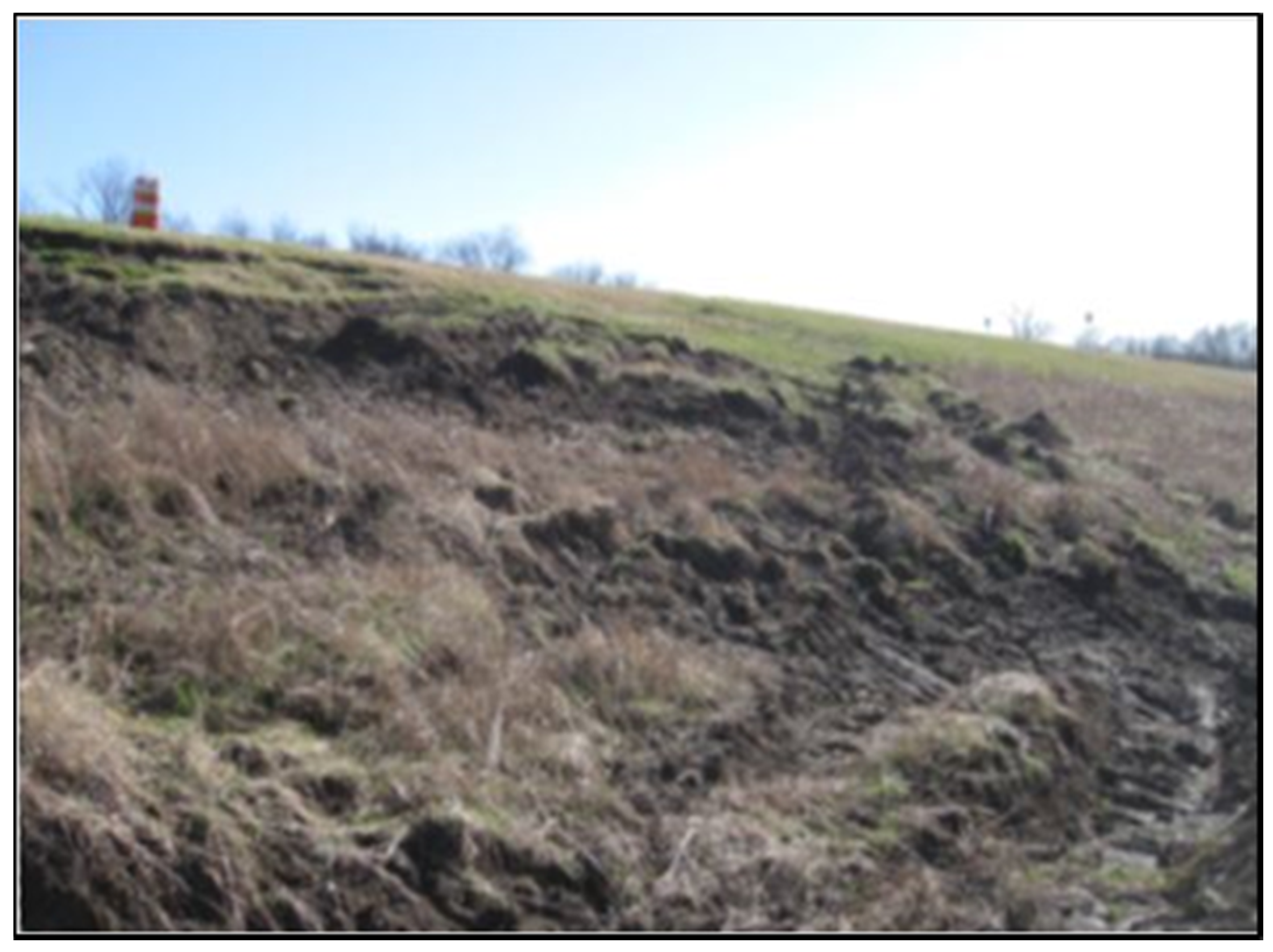
In this paper, we compare the accuracy of the supervised classification methods minimum distance (MD) using Euclidean and Mahalanobis distance, support vector machine (SVM), and maximum likelihood (ML), using SAR technology to detect slough slides on earthen levees. Our motivation for this paper is to compare the performance analysis of several supervised classification methods. SAR technology, due to its high spatial resolution and soil penetration capability, is a good choice to identify such problem areas on levees, so that they can be treated to avoid possible catastrophic failure [1,3]. The roughness and related textural characteristics of the soil in a slide affect the amount and pattern of radar backscatter. The type of vegetation that grows in a slide area differs from the surrounding levee vegetation, which can also be used in detecting slides [4]. An illustration of a slide on a levee is shown in Figure 2.
The remainder of this paper is organized as follows. Section 2 describes materials and methods, which includes data descriptions and methods used in this paper: minimum distance using Euclidean distance, minimum distance using Mahalanobis distance, support vector machine, and maximum likelihood. Section 3 describes results and discussion. Finally, Section 4 offers our conclusions.
2. Materials and Methods
The NASA Jet Propulsion Laboratory’s (JPL’s) uninhabited aerial vehicle SAR (UAVSAR) is a fully polarimetric L-band SAR which is designed to acquire airborne SAR data in a fully quad-polarimetric manner. SAR technology, due to its high spatial resolution and soil penetration capability, the is a good choice to identify such problem areas on levees, so that they can be treated to avoid possible catastrophic failure [1,3]. PolSAR data contain a variety of information which relates to the physical properties of the target. In PolSAR, the transmitted signal is polarized and different polarizations of the backscatter signal are detected with different polarizations, which includes: VV (vertically transmitted and vertically received), HV (horizontally transmitted and vertically received), and HH (horizontally transmitted and horizontally received). HH and VV configurations produce like-polarized radar imagery. HV and VH configurations produce cross-polarized radar imagery. Hence, polSAR provides much more information due to transmitted signal being polarized and different polarizations of the backscatter signal are detected [12]. The L-band SAR measurements can penetrate dry soil to as much as one-meter depth. Thus, they may be valuable in detecting changes in levees that will aid in levee vulnerability classification.
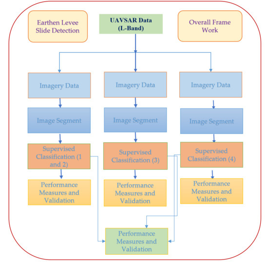
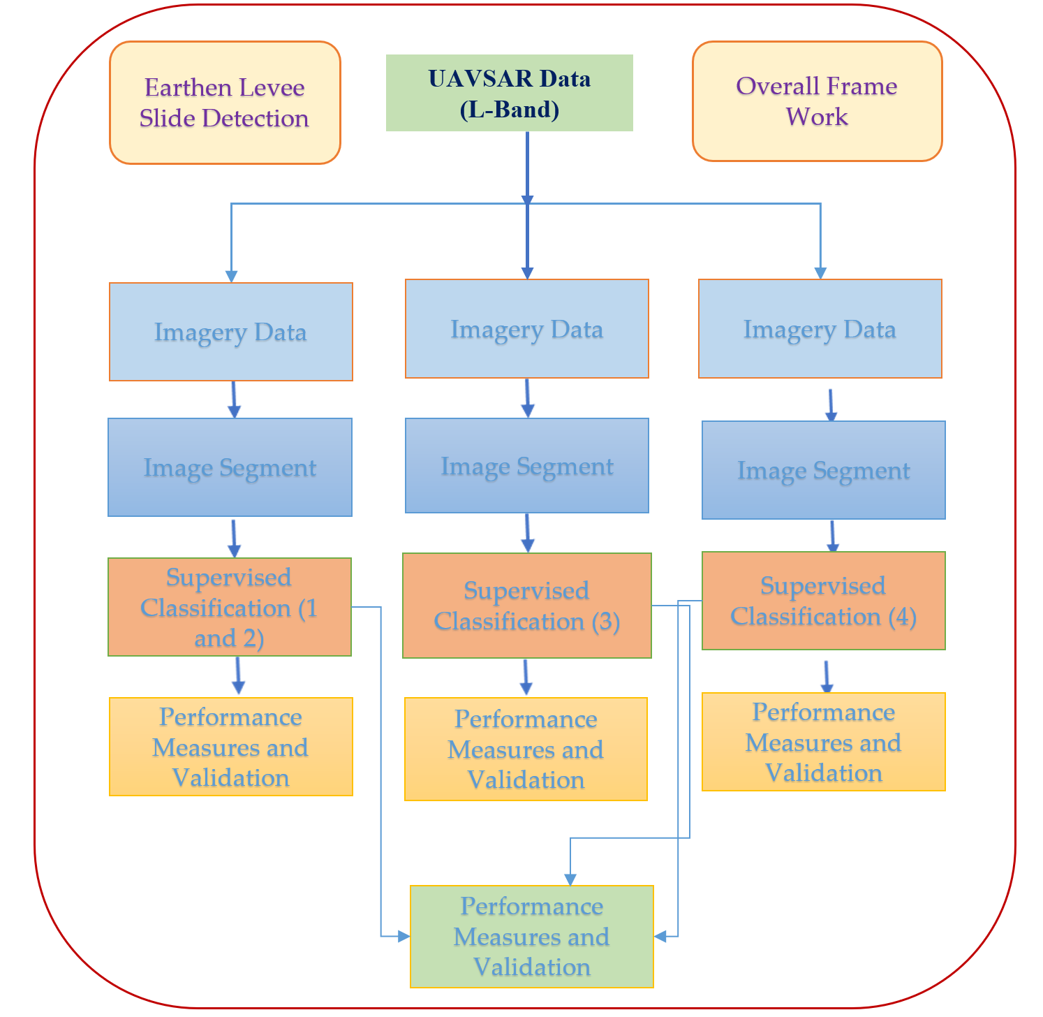
The supervised classification process consists of: selection of SAR sets and data bands, image segmentation of the levee area from the water side toe to the center of the levee, training the supervised classifier with training data, testing the area of interest, and validating the results using ground truth data, as shown in Figure 3.
2.1. Data Description
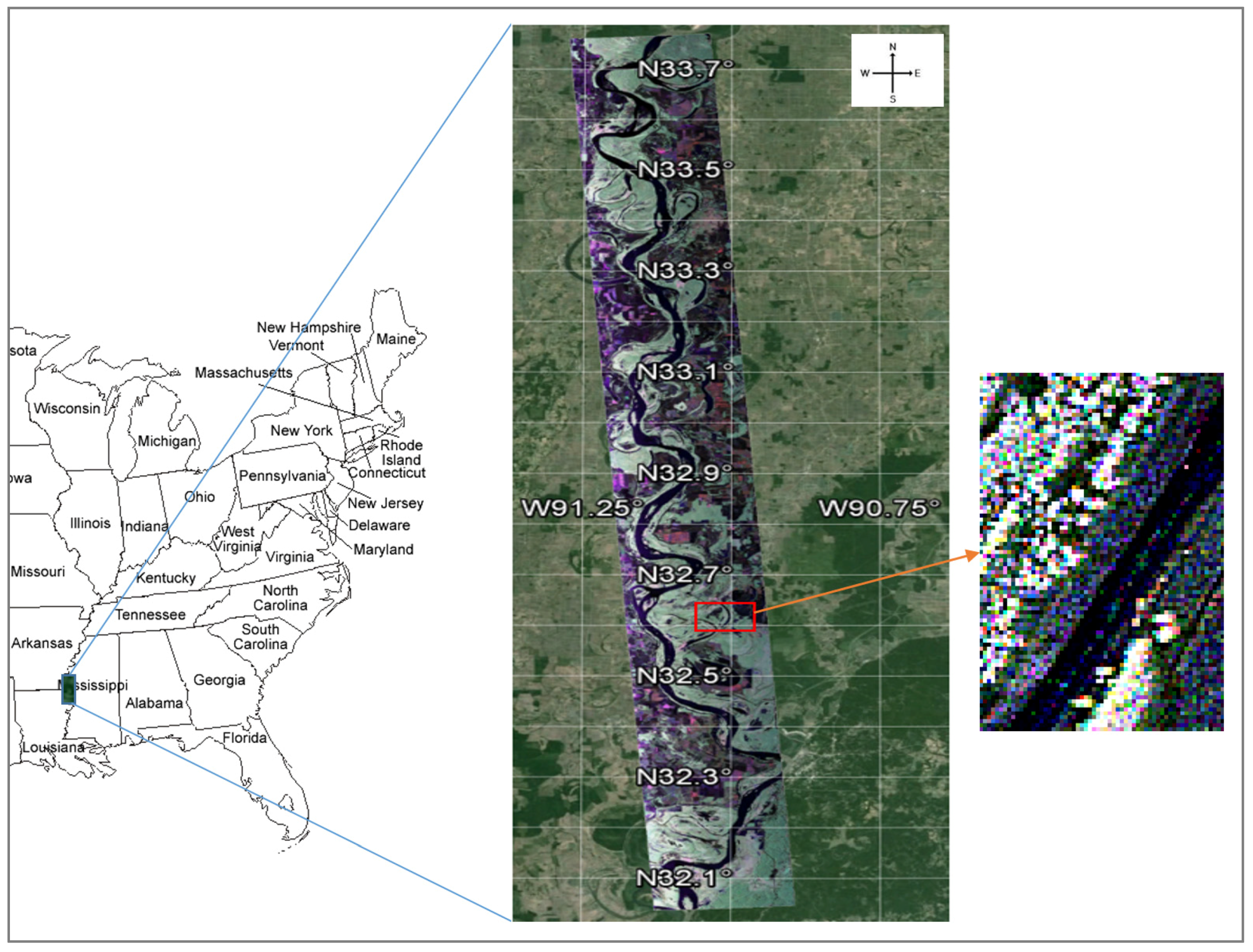
The classification is performed using multi-look cross products (MLC) of the UAVSAR data acquired on 25 January 2010. The MLC datasets are real floating point, four bytes per pixel. These real powers are derived from an average of three pixels in range and 12 pixels in azimuth, i.e., the number of range looks in MLC and number of azimuth looks in MLC are 3 × 12 for each single look complex data (SLC) pixel, which correspond to HHHH, HVHV, and VVVV. Three polarization channels HHHH, HVHV, and VVVV backscatter magnitudes are used as features for the classification. The pixel spacing for the MLC data is by 7.2 m × 4.99 m for the azimuth and range directions, respectively. The pixel spacing for the SLC data is by 0.6 m × 1.66 m for the azimuth and range directions, respectively [11]. The SLC datasets (HH, HV, and VV) are oversampled in nature and are dominated by speckle noise. We chose the MLC datasets to reduce the speckle effects. We choose HHHH, HVHV, and VVVV MLC data. For the MLC data, the projected multi-look data used has a ground sample size of 5.5 m by 5.5 m. UAVSAR projects slant range images to the ground range using the backward projection method. The image segment consists of 61 × 89 × 3 pixels (columns, rows, bands), and covers a 633 m long stretch of levee in the area noticeable with a red color rectangular box on the flight line full segment radar image, overlaid on the base map, as shown in Figure 4. The full image includes the portion of boundaries of Louisiana, Mississippi, and Arkansas states. For the multi-polarized SAR imagery, it is useful to create a color composite image from the HH, HV, and VV channels that are being mapped to red, green, and blue, as shown in Figure 4, which comprises both an overview image as well as a close-up view of the segmented test area. The overview image has a swath width of 20 km and a total length of approximately 200 km. The radar is fully polarimetric with a range bandwidth of 80 MHz (resulting in better than 2 m range resolution) and flies at a nominal altitude of 13,800 m [1].
The river side from the center of the levee is segmented because the probabilities of occurrence of slides are greater there than on the land side, since usually the water side of the levee has steep slope compared with the land side, as we have noticed from our field trips to collect ground truth data. The slope failure is one of the main cause for the occurrence of slides and potential slides. The supervised classification methods are trained with two training classes: slide (i.e., anomalous) and non-slide (i.e., healthy) areas. We used “ground truth” reference data to train and test the classification algorithms. Finally, the overall slide and non-slide accuracies were computed using the confusion matrix. The study area for this work focuses on the mainline levee system of the Mississippi River along the eastern side of the river, in Mississippi, USA.
The availability of ground truth data for training the supervised classification processes for the present application is a challenge since the targets of interest are portions of the levee that show signs of impending failure. Once these are detected, they are quickly repaired depending on their severity [13]. The study area is one in which the levees are managed by the US Army Corps of Engineers (USACE) and are well-monitored. The Corps, in association with the local levee boards, maintains a good cumulative history of past problems and have identified particularly problematic sections of levees in the study area, as shown in Table 1. The ground truth data is provided by USACE with the approximate dates slides appeared, dates slides were repaired, and ground coordinate locations. Ground truth data was also compared to the optical National Agriculture Imagery Program (NAIP) imagery to visually confirm the slide events as unrepaired or repaired. These are used as training samples. In addition to the ground truth data provided by the Corps, we have conducted field trips at the time of image acquisition to visually inspect the slide areas and levee conditions. The active slide (slide 3) was present and unrepaired during the radar image acquisition time on 25 January 2010. Though the date of slide appearance was not identified by the Corps for slide 3, it is visible in the NAIP imagery collected in 2009 and 2010 [14], and was not repaired until after the image acquisition as shown in Table 2. Hence, it was an active slide during the time of the image. Training masks were created for the slide events and labeled as either repaired or unrepaired at the time of acquisition. The training sample data from slide and non-slide (healthy) parts of the levees were obtained from the radar data using the training masks for analysis. The samples from the healthy parts of the levee near the slide events were used for training of the non-slide (healthy levee) class.
2.2. Methods
2.2.1. Minimum Distance Using Euclidean Distance
Minimum distance classification uses the mean vectors for each class and calculates the Euclidean distance from each unknown pixel to the mean vector for each class. The pixels are classified to the nearest class [15]. The standard deviations from mean can be no threshold, single value, or multiple values. The lower the threshold value, the more pixels that are unclassified. The maximum distance error can be no threshold, single value or multiple values. The smaller the distance threshold, the more pixels that are unclassified. The pixel of interest must be within both the threshold for distance to the mean and the threshold for the standard deviation for a class. The classification is performed with zero standard deviation from the mean, and zero maximum distance error, to classify all pixels. Minimum distance classification calculates the Euclidean distance for each pixel in the image to each class [15]:
where,
- D = Euclidean distance
- i = the ith class
- x = n-dimensional data (where n is the number of features)
- mi = mean vector of a class
2.2.2. Minimum Distance Using Mahalanobis Distance
The Mahalanobis distance is a direction-sensitive distance classifier that uses statistics for each class in a manner like the maximum likelihood classifier. However, it assumes all class covariances are equal. Therefore it is a faster method and weighing factors are not required [15]. All pixels are classified to the closest training data. It is largely based on a normal distribution of the data in each band which is used as input to classification. The maximum distance error can be a zero threshold for all the classes, or single value for all the classes, or different values for individual classes. The distance threshold is the distance within which a class must fall from the center or mean of the distribution for a class. We used a zero threshold for all the classes and zero maximum distance error, to classify all pixels. The Mahalanobis distance classification calculates the distance for each pixel in the image to each class using the following equation [15]:
where:
- D = Mahalanobis distance
- i = the ith class
- x = n-dimensional data (where n is the number of features)
- Σ−1 = the inverse of the covariance matrix of a class
- = mean vector of a class
2.2.3. Support Vector Machine
Support vector machine (SVM) is a supervised classification method derived from statistical learning theory that often yields good classification results from complex and noisy data [15,16,17,18]. SVM separates the classes with a decision surface that maximizes the margin between the classes [19]. The benefit of SVM is that it works well with small training datasets. A kernel type must be selected for use in the SVM classifier. These kernels show a critical role in SVM classification. The kernel types are linear, polynomial, radial basis function, and sigmoid. If the kernel type is polynomial, we need to choose the degree of the kernel polynomial. If the kernel type is polynomial or sigmoid, we need to specify the bias in the kernel function. If the kernel type is polynomial, radial basis function, or sigmoid, we must also specify a gamma value which defines how far the influence of a single training sample reaches [19]. The kernel type used here is a radial basis function. Gamma in the kernel function used is 0.333 (ideally the gamma value is the inverse of bands used in the input image, the number of bands used in this data, were 3. So, 1/3 = 0.333). The penalty parameter, which controls the trade-off between allowing training errors and forcing rigid margins, used is 100. The pyramid levels, which set the number of hierarchical processing levels to apply during the SVM training and classification process, used is 0.00, to process the images at full resolution. We use the classification probability threshold to set the probability that is required for the SVM classifier to classify a pixel. The classification probability threshold used is zero, to classify all pixels.
2.2.4. Maximum Likelihood
Maximum likelihood assumes that the statistics for each class in each band are normally distributed and calculates the probability that a given pixel belongs to a specific class. Each pixel is assigned to the class that has the highest probability (i.e., the maximum likelihood) [15]. The threshold is a probability minimum for inclusion in a class. We used a zero threshold for all the classes to classify all pixels. Maximum likelihood classification calculates the following discriminant functions for each pixel in the image:
where:
- i = the ith class
- x = n-dimensional data (where n is the number of features)
- p(ωi) = probability that a class occurs in the image and is assumed the same for all classes
- |Σi| = determinant of the covariance matrix of the data in a class
- Σi−1 = the inverse of the covariance matrix of a class
3. Results and Discussion
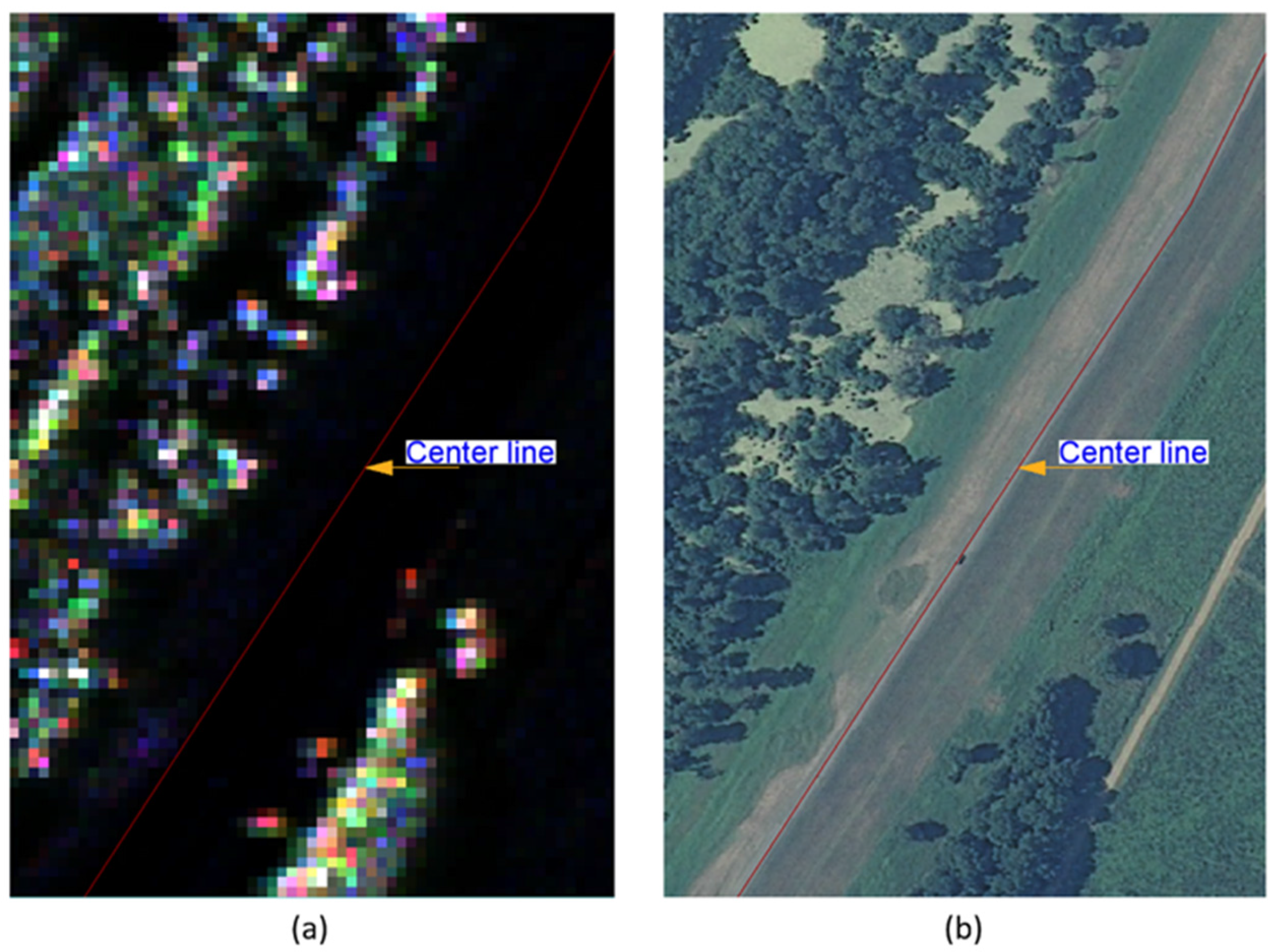
The minimum distance (MD) using Euclidean and Mahalanobis distance, support vector machine (SVM), and maximum likelihood (ML) supervised classification processes were run separately, with the polSAR multi-looked cross product data. The test study area SAR image and corresponding geographically-located optical image, overlaid with the levee center line, are shown in Figure 5. Using the ground truth data, image masks were created bounding the active slide area and a subset of the non-slide area within segmented image (i.e., test area), as shown in Figure 6. A sample of the pixels in of each of these two classes was then used to train all four supervised classifiers. The accuracy of the resulting classification was tested using the remaining reference data pixels for testing, and the conventional statistics of user, producer, and overall accuracy were computed for each method (in the form of percentages as well as pixel) using the confusion matrix.
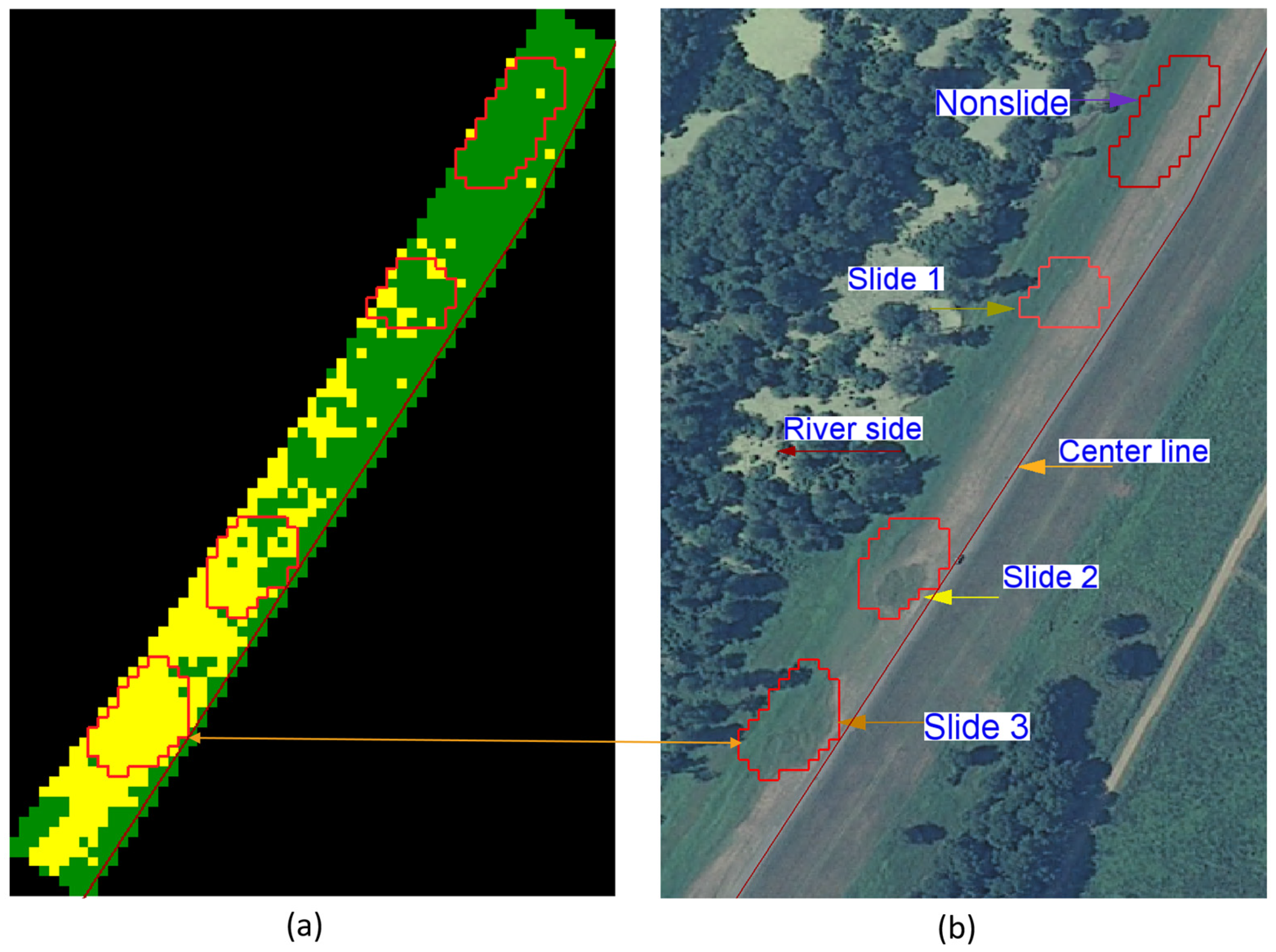
The classification maps resulting from applying the MD using Euclidean and Mahalanobis distance, SVM, and ML classification to test areas using co-polarized features (HHHH, HVHV, VVVV), are shown in Figure 7, Figure 8 and Figure 9. The training masks are shown in Figure 6b for both slide and non-slide classes. The accuracy assessment results for all four classifiers are tabulated in Table 3. The summary of accuracy assessment results which include overall accuracy, slide accuracy, and non-slide accuracy are listed in the Table 4. The training masks, shown in Figure 6b, cover 78 and 84 pixels for the slide and non-slide area, respectively. Total pixels of the testing area (as shown in Figure 6a) were 929. Of these, 17% (162 pixels) were used for training the classifier and the remainder used for testing its accuracy. All 4 supervised classification results show good detection of the slide areas, but numerous false positive detections as well. The test area included one active slide and two slides (numbered 1 and 2, as shown in Figure 9) which had been repaired by the time of image acquisition. Many of the false positive pixels fall in this repaired area. Since these slide areas were repaired only two months prior to the time of image acquisition, they still have characteristics more like the active slide than the “healthy” areas in terms of surface roughness and differences in the grass cover. These characteristics likely influenced the classification. Out of these two repaired slides, the slide 2 area has more false positives, since it appeared in August 2008, and was repaired in November 2009. To the contrary, the slide 1 area has fewer false positives since it appeared in October 2009, and was repaired in November 2009. Hence, the slide 2 areas might contain more surface roughness and differences in the grass cover. The classification accuracies obtained for all four methods are quite high. The ML results are the best, followed by SVM, and MD using Mahalanobis and Euclidean distance. All four methods achieved near-perfect identification of non-slide pixels, but differ in the detection of slide pixels (thus, in their false positive results, identifying some non-slide pixels as slides). In addition to the active slide areas, other anomalous areas are also detected to some degree and classified into the slide class. Some of these are previous slide areas that had been repaired just two months prior to the time of image acquisition and still appear similar enough to the active slide to be detected by the classification technique.
4. Conclusions
Supervised classification methods based on the minimum distance (MD) using Euclidean and Mahalanobis distance, support vector machine (SVM), and maximum likelihood (ML) classification for earthen levee slide detection using UAVSAR imagery were presented. The effectiveness of the algorithms is demonstrated using fully quad-polarimetric L-band SAR imagery from the NASA JPL’s UAVSAR. Three polarization channels HHHH, HVHV, and VVVV back-scatter magnitudes are used as features for all four supervised classification methods. The study area is a section of the lower Mississippi River valley in the Southern USA. The classification results obtained for all four procedures indicate that the use of polarimetric SAR can effectively detect slide areas on earthen levees. The overall performance of the ML classification was the best, but all had quite good accuracy. The SVM method is somewhat more complicated to implement than the other two methods, involving more parameters and options which must be specified. Although the test study area is small, including only one active slide area and two anomalous areas for testing, the methodologies presented in this paper show promising results. Planned future work includes the use of larger test areas consisting of more active slides, seasonal images acquired by the SAR, and different geometrical orientations of the levee.
Acknowledgments
This work was supported by the National Science Foundation grant number: OISE-1243539, and by the NASA Applied Sciences Division under grant number: NNX09AV25G. The authors would like to thank the US Army Corps of Engineers, Engineer Research and Development Center and Vicksburg Levee District for providing ground truth data and expertise; NASA Jet Propulsion Laboratory for providing the UAVSAR image.
Author Contributions
Ramakalavathi Marapareddy implemented the classification methods. James V. Aanstoos supervised the work, provided imagery and data, and was the principal investigator for the project. Nicolas H. Younan supervised and provided guidance. Ramakalavathi Marapareddy, James V. Aanstoos, and Nicolas H. Younan analyzed the results and wrote the paper.
Conflicts of Interest
The authors declare no conflict of interest.
References
- Aanstoos, J.V.; Hasan, K.; O’Hara, C.G.; Prasad, S.; Dabbiru, L.; Mahrooghy, M.; Nobrega, R.; Lee, M.L.; Shrestha, B. Use of Remote Sensing to Screen Earthen Levees. In Proceedings of the 39th IEEE Applied Imagery Pattern Recognition Workshop, Washington, DC, USA, 13–15 October 2010; pp. 1–6. [Google Scholar]
- Dunbar, J. USACE’s lower Mississippi valley engineering geology and geomorphology mapping program for levees. In Presentation at Vicksburg; USACE: Vicksburg, MS, USA, 16 April 2009. [Google Scholar]
- Aanstoos, J.V.; Hasan, K.; O’Hara, C.; Prasad, S.; Dabbiru, L.; Mahrooghy, M.; Gokaraju, B.; Lee, M.; Nobrega, R.A.A. Earthen Levee Monitoring with Synthetic Aperture Radar. In Proceedings of the 2011 IEEE Applied Imagery Pattern Recognition Workshop (AIPR), Washington, DC, USA, 11–13 October 2011. [Google Scholar]
- Hossain, A.K.M.A.; Easson, G.; Hasan, K. Detection of Levee Slides Using Commercially Available Remotely Sensed Data. Environ. Eng. Geosci. 2006, 12, 235–246. [Google Scholar] [CrossRef]
- MS Levee Board. Available online: http://www.msleveeboard.com/index.php/about/history (accessed on 3 July 2017).
- Knoeff, H.; Vastenburg, W.E. Automated Engineering in Levee Risk Management. In Proceedings of the 3rd International Symposium on Geotechnical Safety and Risk, Munich, Germany, 2–3 June 2011. [Google Scholar]
- USACE. 2012. National Levee Database-Home. Available online: http://nld.usace.army.mil/egis/f?p=471:1 (accessed on 4 July 2017).
- The Mississippi River & Tributaries Project: Levee System Evaluation Report for the National Flood Insurance Program. April 2014. Available online: http://www.mvd.usace.army.mil/Portals/52/docs/MRC/LeveeSystem/MRT_levee_system_eval_report_for_NFIP.pdf (accessed on 7 October 2017).
- Kong, J.A.; Yueh, S.H.; Lim, H.H.; Shin, R.T.; van Zyl, J.J. Classification of earth terrain using polarimetric synthetic aperture radar images. Progress Electromagn. Res. 1990, 3, 327–370. [Google Scholar]
- Pottier, E.; Lee, J.-S.; Ferro-Famil, L. PolSARpro 4.2 (Polsarpro is a Polarimetric SAR Data Processing and Educational Tool). Available online: http://polsarpro.software.informer.com/4.2/ (accessed on 7 October 2017).
- Marapareddy, R.; Aanstoos, J.V.; Younan, N.H. A Supervised Classification Method for Levee Slide Detection using Complex Synthetic Aperture Radar Imagery. J. Imaging 2016, 2, 26. [Google Scholar] [CrossRef]
- Aanstoos, J.V. Levee Assessment via Remote Sensing; SERRI Report 80023-02; Southeast Region Research Initiative: Oak Ridge, TN, USA, 2012. [Google Scholar]
- Aanstoos, J.V.; Hasan, K.; O’Hara, C.; Dabbiru, L.; Mahrooghy, M.; Nobrega, R.A.A.; Lee, M.M. Detection of Slump Slides on Earthen Levees Using Polarimetric SAR Imagery. In Proceedings of the 2012 IEEE Applied Imagery Pattern Recognition Workshop, Washington, DC, USA, 9–11 October 2012. [Google Scholar]
- Uninhabited Aerial Vehicle Synthetic Aperture Radar. Available online: http://www.jpl.nasa.gov/missions/index.cfm?mission=UAVSAR (accessed on 10 July 2017).
- ENVI Version 5.1. Exelis Visual Information Solutions User Guides and Tutorials. Available online: http://www.exelisvis.com/Learn/Resources/Tutorials.aspx (accessed on 15 July 2017).
- Soliman, O.S.; Mahmoud, A.S. A classification system for remote sensing satellite images using support vector machine with non-linear kernel functions. In Proceedings of the 8th International Conference on Informatics and Systems (INFOS), Cairo, Egypt, 14–16 May 2012; pp. 181–187. [Google Scholar]
- Kaya, G.T.; Ersoy, O.K.; Kamasak, M.E. Support Vector Selection and Adaptation for Remote Sensing Classification. IEEE Trans. Geosci. Remote Sens. 2011, 49, 2071–2079. [Google Scholar] [CrossRef]
- Morton, J.C. Image Analysis, Classification and Change Detection in Remote Sensing: With Algorithms for ENVI/IDL and Python 2014, 3rd ed.; CRC Press: Boca Raton, FL, USA, 2014; pp. 1–576. ISBN 9781466570375. [Google Scholar]
- Hsu, C.-W.; Chang, C.-C.; Lin, C.-J. A Practical Guide to Support Vector Classification. National Taiwan University, 2010. Available online: http://ntu.csie.org/~cjlin/papers/guide/guide.pdf (accessed on 15 July 2017).
Figure 1.
Earthen levee at Eagle Lake, Warren County, Vicksburg, MS, USA.
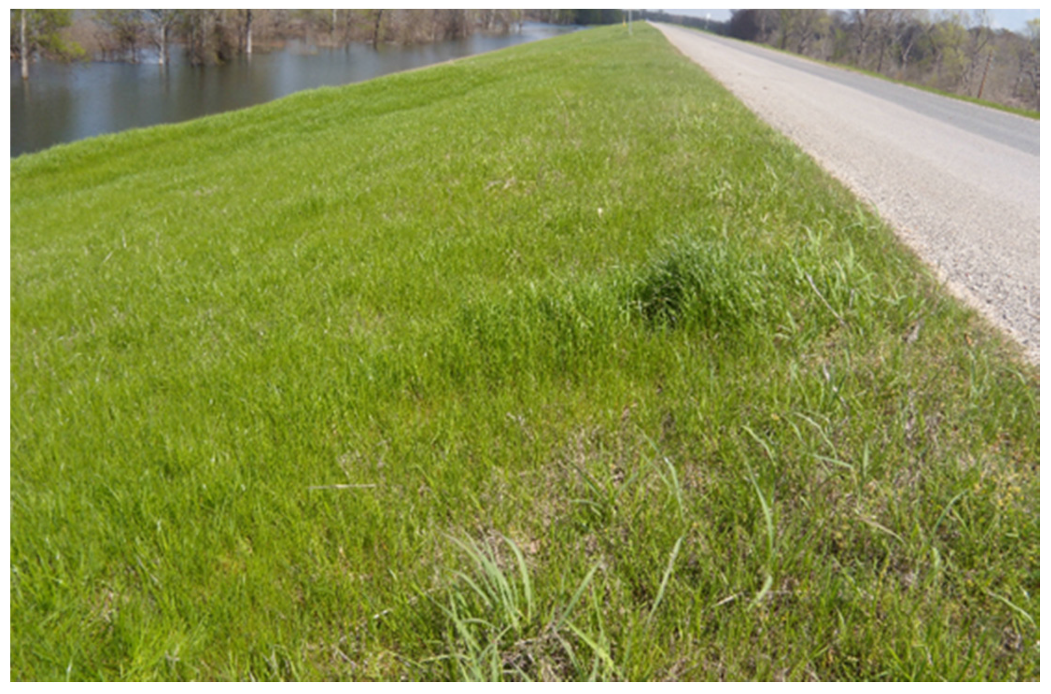
Figure 2.
Slough or slump slide on a levee.

Figure 3.
Supervised classification workflow for slide detection on levee.
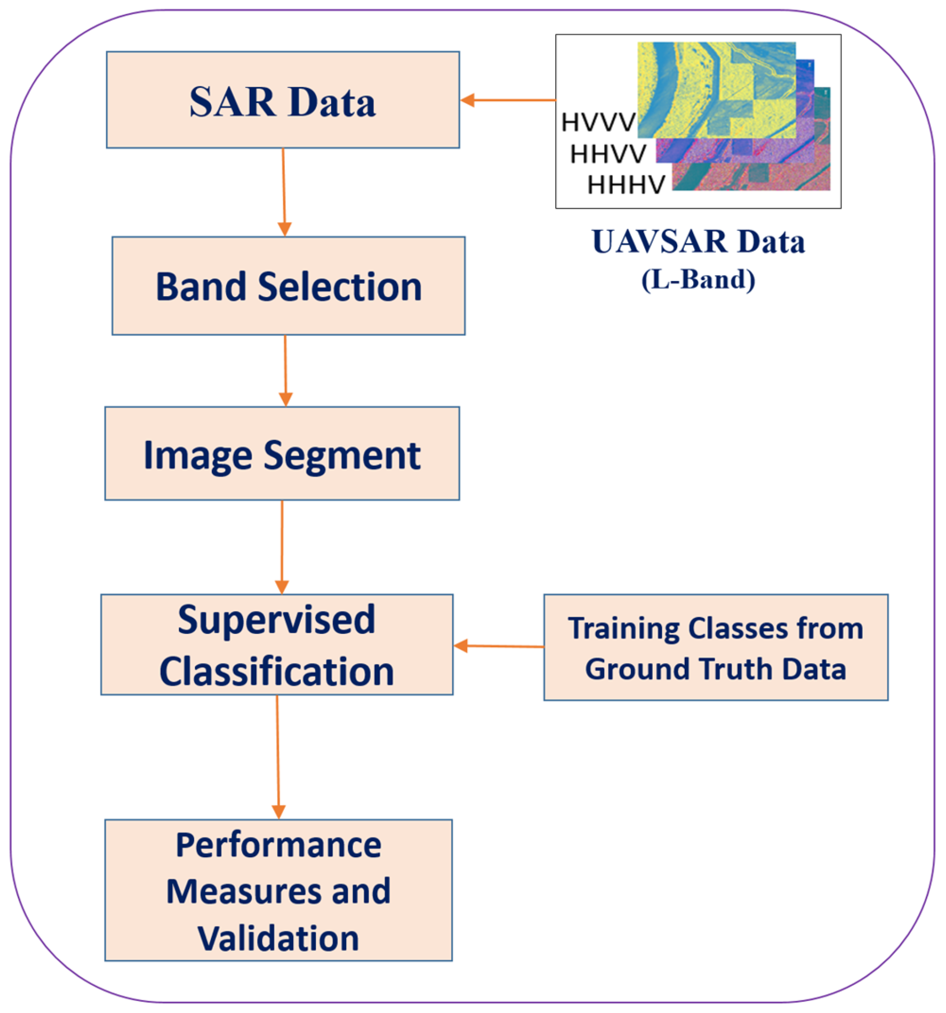
Figure 4.
Study area with a radar color composite three-band (HH, VV, and HV) image overlaid on a base map.
Figure 4.
Study area with a radar color composite three-band (HH, VV, and HV) image overlaid on a base map.

Figure 5.
(a) Test area SAR image; and (b) optical image; overlaid with the levee center line.

Figure 6.
(a) Segmented test area SAR image; and (b) classification training classes; overlaid with the levee center line.
Figure 6.
(a) Segmented test area SAR image; and (b) classification training classes; overlaid with the levee center line.
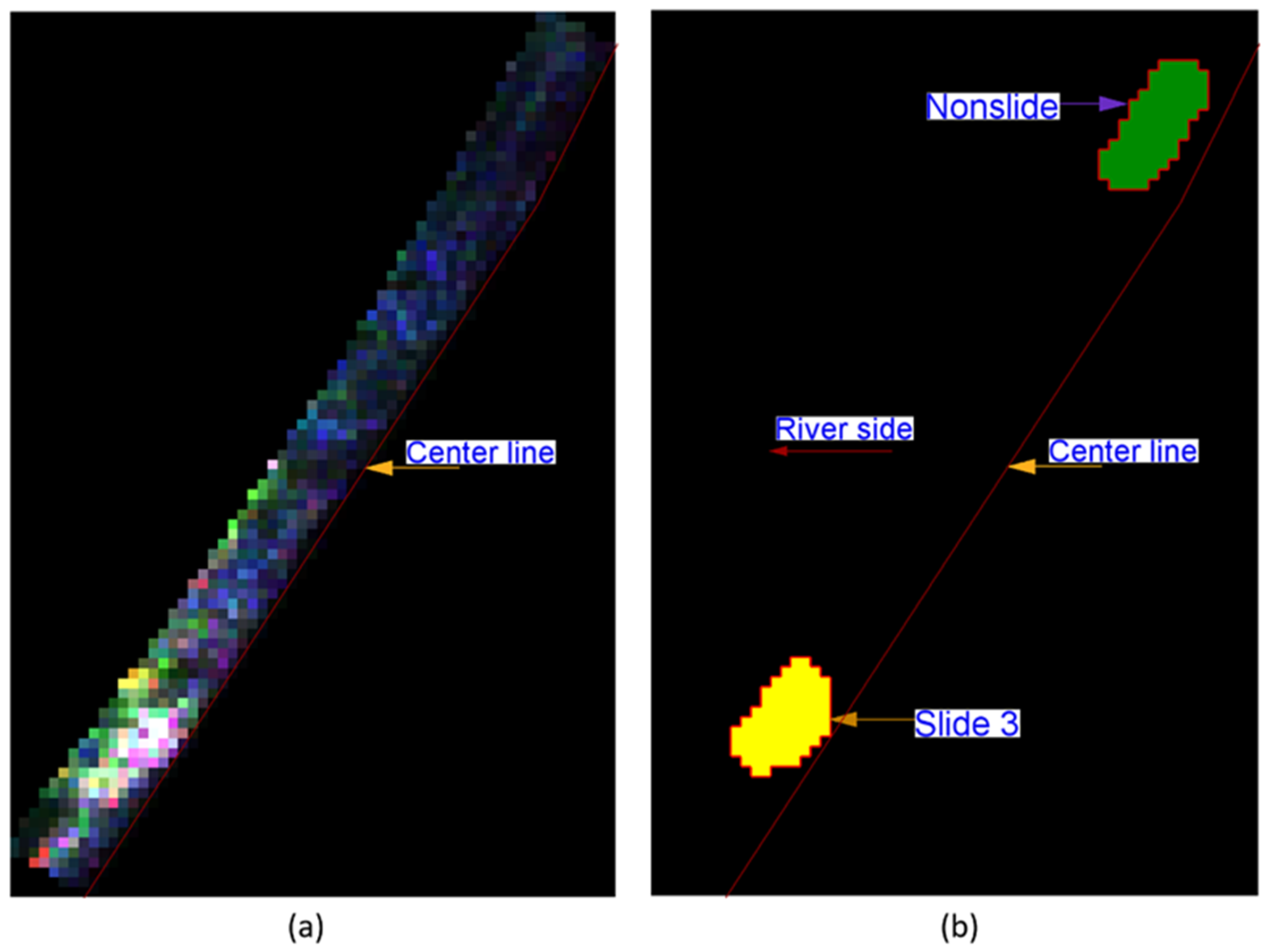
Figure 7.
Minimum distance classification, using: (a) Euclidean distance; and (b) Mahalanobis distance.
Figure 7.
Minimum distance classification, using: (a) Euclidean distance; and (b) Mahalanobis distance.
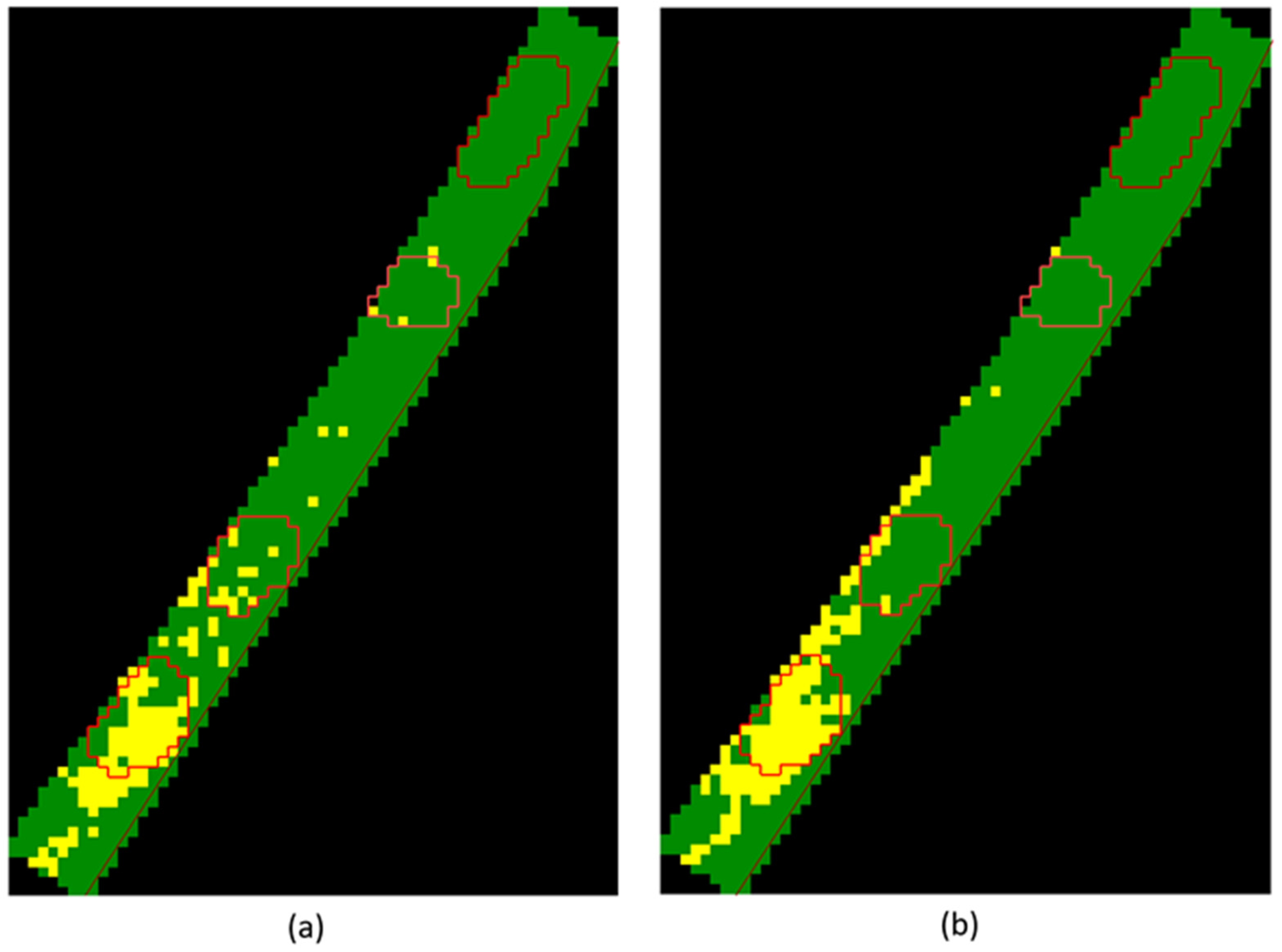
Figure 8.
(a) Support vector machine classification; and (b) maximum likelihood classification.
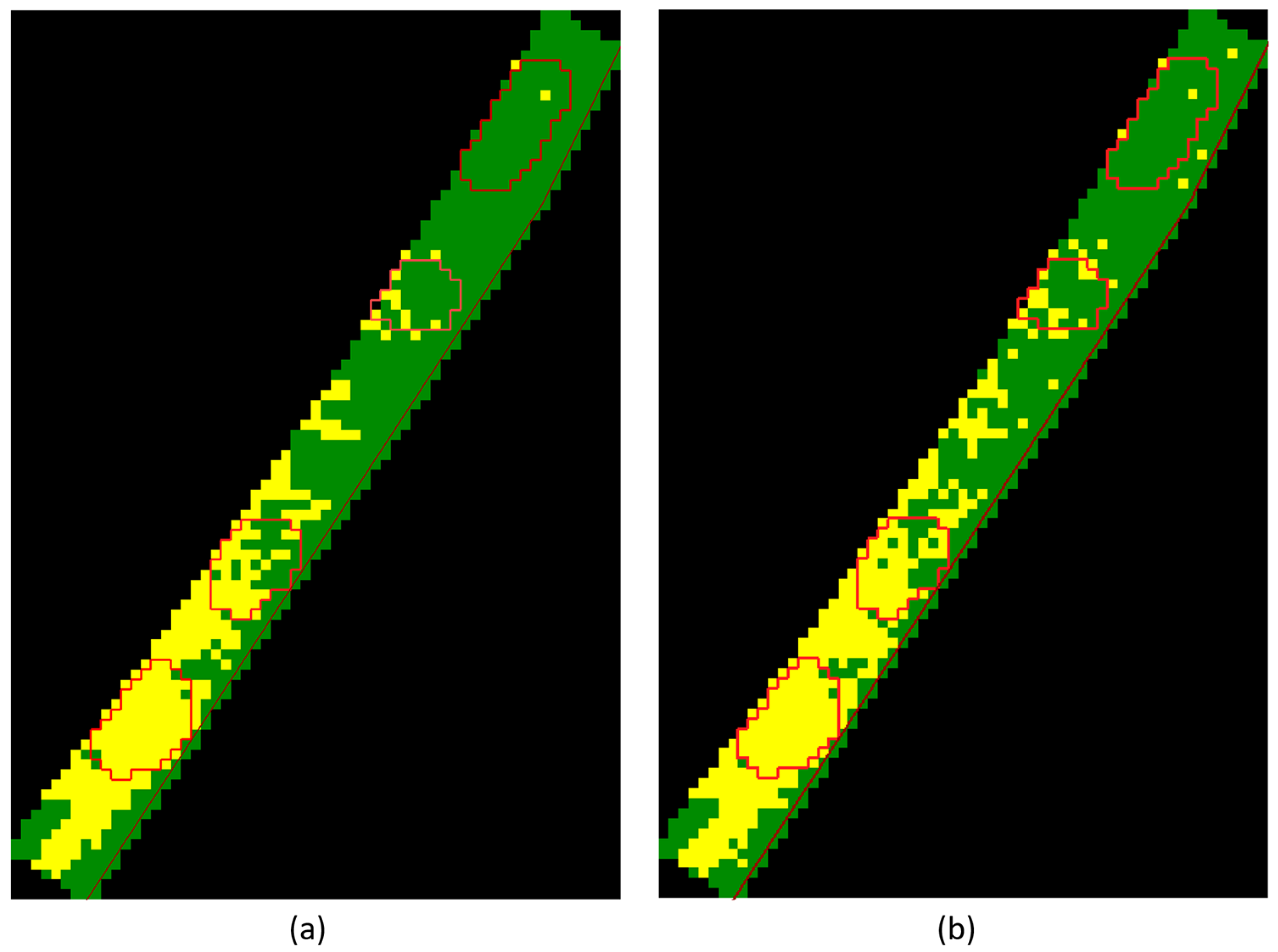
Figure 9.
(a) Maximum likelihood classification; and (b) optical image; overlaid with the levee center line, slide, and non-slide areas.
Figure 9.
(a) Maximum likelihood classification; and (b) optical image; overlaid with the levee center line, slide, and non-slide areas.

Table 1.
Ground truth data from the Mississippi Levee Board.
| Slide Number | Length | Vert. Face | Dist. from Crown | Latitude North | Longitude West | Date Slide Appeared | Date Slide Repaired |
|---|---|---|---|---|---|---|---|
| 1 | 80’ | 2’ | 30’ | N 32-36’-37.7” | W 90-59’-42.3” | Oct. 2009 | Nov. 2009 |
| 2 | 120’ | 3’ | 15’ | N 32-36’-32.0” | W 90-59’-46.3” | Aug. 2008 | Nov. 2009 |
| 3 | 200’ | 8’ | 8’ | N 32-36’-29.1” | W 90-59’-48.0” | - | Sept. 2010 |
Table 2.
Updated slides ground truth from the Mississippi Levee Board.
| Slide No. | From Levee Board (8 April 2011) | From Visual Aerial Photo Inspection | ||
|---|---|---|---|---|
| Date Slide Appeared | Date Slide Repaired | NAIP 2009 (May–Sep.) | NAIP 2010 (May–Sep.) | |
| 1 | Oct. 2009 | Nov. 2009 | Not Visible (July 25) | Repaired (June 22) |
| 2 | Aug. 2008 | Nov. 2009 | Unrepaired (July 25) | Repaired (June 22) |
| 3 | - | Sept. 2010 | Unrepaired (July 25) | Unrepaired (June 22) |
Table 3.
Accuracy analysis of the MD using Euclidean and Mahalanobis distance, SVM, and ML classification, for the slide and non-slide areas.
Table 3.
Accuracy analysis of the MD using Euclidean and Mahalanobis distance, SVM, and ML classification, for the slide and non-slide areas.
| Classification Method V/s. Accuracy (%) | Overall Accuracy = (132/162) 81% | ||||||||
|---|---|---|---|---|---|---|---|---|---|
| Ground Truth (Pixels) | Ground Truth (%) | ||||||||
| MD u/Euclidean | Class | slide3 | non-slide | Total | slide3 | non-slide | Total | Prod. Accu. (%) | User Accu. (%) |
| slide3 | 48 | 0 | 48 | 61 | 0 | 29 | 61 | 100 | |
| non-slide | 30 | 84 | 114 | 38 | 100 | 70 | 100 | 73 | |
| Total | 78 | 84 | 162 | 100 | 100 | 100 | |||
| MD u/Mahalanobis | Overall Accuracy = (146/162) 90% | ||||||||
| slide3 | 62 | 0 | 62 | 79 | 0 | 38 | 79 | 100 | |
| non-slide | 16 | 84 | 100 | 20 | 100 | 61 | 100 | 84 | |
| Total | 78 | 84 | 162 | 100 | 100 | 100 | |||
| SVM | Overall Accuracy = (158/162) 97% | ||||||||
| slide3 | 62 | 0 | 62 | 79 | 0 | 38 | 96 | 98 | |
| Non-slide | 16 | 84 | 100 | 20 | 100 | 61 | 98 | 96 | |
| Total | 78 | 84 | 162 | 100 | 100 | 100 | |||
| ML | Overall Accuracy = (159/162) 98% | ||||||||
| slide3 | 76 | 1 | 77 | 97 | 1 | 47 | 97 | 98 | |
| non-slide | 2 | 83 | 85 | 2 | 98 | 52 | 98 | 97 | |
| Total | 78 | 84 | 162 | 100 | 100 | 100 | |||
Note: Accu. ≥ Accuracy; Prod. ≥ Producer; u/Euclidean ≥ using Euclidean; u/Mahalanobis ≥ using Mahalanobis.
Table 4.
Accuracy analysis of the MD using Euclidean and Mahalanobis distance, SVM, and ML classification, for the slide and non-slide areas.
Table 4.
Accuracy analysis of the MD using Euclidean and Mahalanobis distance, SVM, and ML classification, for the slide and non-slide areas.
| Classification Method Vs. Accuracy (%) | Overall Accuracy | Slide Accuracy | Non-slide Accuracy | |
|---|---|---|---|---|
| MD | u/Euclidean | 81 | 61 | 100 |
| u/Mahalanobis | 90 | 79 | 100 | |
| SVM | 97 | 96 | 98 | |
| ML | 98 | 97 | 98 | |
© 2017 by the authors. Licensee MDPI, Basel, Switzerland. This article is an open access article distributed under the terms and conditions of the Creative Commons Attribution (CC BY) license (http://creativecommons.org/licenses/by/4.0/).
Share and Cite
MDPI and ACS Style
Marapareddy, R.; Aanstoos, J.V.; Younan, N.H. Accuracy Analysis Comparison of Supervised Classification Methods for Anomaly Detection on Levees Using SAR Imagery. Electronics 2017, 6, 83. https://doi.org/10.3390/electronics6040083
AMA Style
Marapareddy R, Aanstoos JV, Younan NH. Accuracy Analysis Comparison of Supervised Classification Methods for Anomaly Detection on Levees Using SAR Imagery. Electronics. 2017; 6(4):83. https://doi.org/10.3390/electronics6040083
Chicago/Turabian StyleMarapareddy, Ramakalavathi, James V. Aanstoos, and Nicolas H. Younan. 2017. "Accuracy Analysis Comparison of Supervised Classification Methods for Anomaly Detection on Levees Using SAR Imagery" Electronics 6, no. 4: 83. https://doi.org/10.3390/electronics6040083
Note that from the first issue of 2016, this journal uses article numbers instead of page numbers. See further details here.