A Microcontroller-Based Adaptive Model Predictive Control Platform for Process Control Applications


1
School of Science, Engineering and Design, Teesside University, Middlesbrough, TS1 3BA, UK
2
School of Health and Social Care, Teesside University, Middlesbrough, TS1 3BA, UK
*
Author to whom correspondence should be addressed.
Electronics 2017, 6(4), 88; https://doi.org/10.3390/electronics6040088
Submission received: 15 September 2017
/
Revised: 10 October 2017
/
Accepted: 15 October 2017
/
Published: 21 October 2017
Abstract
:Model predictive control (MPC) schemes employ dynamic models of a process within a receding horizon framework to optimize the behavior of a process. Although MPC has many benefits, a significant drawback is the large computational burden, especially in adaptive and constrained situations. In this paper, a computationally efficient self-tuning/adaptive MPC scheme for a simple industrial process plant with rate and amplitude constraints on the plant input is developed. The scheme has been optimized for real-time implementation on small, low-cost embedded processors. It employs a short (2-step) control horizon with an adjustable prediction horizon, automatically tunes the move suppression (regularization) parameter to achieve well-conditioned control, and presents a new technique for generating the reference trajectory that is robust to changes in the process time delay and in the presence of any inverse response. In addition, the need for a full quadratic programming procedure to handle input constraints is avoided by employing a quasi-analytical solution that optimally fathoms the constraints. Preliminary hardware-in-the-loop (HIL) test results indicate that the resulting scheme performs well and has low implementation overhead.
1. Introduction
The potential benefits that adaptive and predictive control schemes can bring to industrial control applications have been well documented in recent years [1,2,3,4,5]. Model predictive control (MPC) schemes employ dynamic models of a process—in conjunction with the use of on-line optimization—to compute an optimal sequence of input moves that minimizes the predicted future values of an objective function [1,2,3]. Most modern MPC schemes utilize a quadratic (2-norm) objective function, with the optimization solved on-line by quadratic programming (QP) software; however, much of the original work on MPC algorithms utilized linear (1-norm) objective functions which were solved on-line by linear programming (LP) software [5,6]. This transition was principally due to a number of well-documented drawbacks to the use of LP in early formulations in MPC, including possible idle/deadbeat dichotomous behaviors, the need to use iterative schemes to obtain solutions even in the unconstrained case, and potentially poor scaling in the size of the MPC problem to the corresponding LP [1,5,6]. MPC generally employs the receding-horizon approach, in which the first control in this sequence is applied, and the optimization is again carried out at the next time step with accurate knowledge of the new state that the process has evolved into. When used with on-line parameter estimation schemes, adaptive MPC becomes a powerful (albeit computationally demanding) control solution, which is well suited to optimal control of industrial plant. The principal components of a typical adaptive MPC implementation are as shown in Figure 1 and consist of an online parameter estimator, adaption mechanism, a predictor of the process future behavior given the (known) current state, and an optimizer (which may have input, output, or state constraints to navigate through).
This paper is concerned with the development of an efficient real-time implementation of input constrained, self-tuning/adaptive MPC algorithm of the generalized predictive control (GPC) type [3] for processes that may be approximated by a second-order plus dead time (SOPDT) dynamic model with or without zeros (either minimum or on-minimum phase). Although this may at first seem somewhat restrictive, research has shown that a large class of open-loop stable processes (such as heating, ventilation, and air conditioning (HVAC), air-fuel ratio control in automobiles, and many pressure and flow applications) can be well approximated by such low-order models [1,2,3,4,5,6]. Indeed, obtaining a simple first- or second-order model forms the first step in most classical PID tuning procedures, such as Ziegler–Nichols, Cohen–Coon, and so on [1,4].
The major drawback of such a scheme is the large computational burden that results especially in constrained and/or adaptive situations. In addition, a typical MPC controller has many tunable parameters: aside from considerations regarding the process parameterization, the principal ones of interest are the choice of sampling time T, the length of the prediction horizon P and the control horizon M, and the value of the move suppression coefficient λ [7,8]. The latter parameter applies a weight on the magnitude of the projected control moves in the objective function. Due to the complex relationships between these tunable parameters and the closed loop system properties, many previous authors have suggested ‘tuning rules’ that allow a user to configure an MPC instance to achieve a desired level of closed-loop performance [7,8]. Taken together, these complications have typically limited the applicability of MPC to situations in which either the required high-bandwidth real-time computing facilities can be justified (or the sampling rate is made appropriately slow), and expert operators are available to help determine an accurate process model and to configure and tune the MPC controller [1,2,3].
In this paper, a computationally efficient self-tuning/adaptive MPC scheme for general industrial process plant is developed. The scheme has been optimized for real-time implementation on small, low-cost embedded processors and is efficient enough to be hosted on a small microcontroller platform (e.g., Arduino, ARM), and features very few tunable parameters. An automatically updated reduced-order process model is employed, along with a two-step control horizon. Rate and amplitude constraints on the plant input are easily fathomed within this framework; CPU time and memory efficiency is achieved by extending previous work to obtain a quasi-analytical solution to optimize over this short constraint horizon and avoid the need for a fully-fledged quadratic programming (QP) procedure. The move suppression coefficient is also automatically tuned to ensure that the controller is well conditioned for the chosen length of prediction horizon. Finally, a new technique to generate a reference trajectory that is robust to changes in the process time delay and in the presence of any inverse response is presented. Although some flexibility in the overall MPC configuration is inevitably lost, the scheme was specifically designed to perform well in industrial process control applications. Preliminary simulation and hardware-in-the-loop-based experimental results indicate that the resulting control is high-performance even when multiple rate and amplitude constraints are active and requires low implementation overhead. The remainder of this paper is structured as follows. Section 2 provides a brief review of previous work in the area of real-time constrained control. Section 3 describes the details of the controller that has been developed. Section 4 describes a series of hardware-in-the-loop (HIL) tests, which have been carried out to investigate and validate the controller. Section 5 provides conclusions.
2. Previous Work
In this section, a short summary is provided of previous work related to the development of efficient techniques for implementing input-constrained optimal control and its real-time implementation. In theory, when an online optimal control features input constraints, a constrained optimization problem of infinite size must be solved at each time step. However, recent results (e.g., refer to [9] and the references therein) have shown that the constraints may be relaxed for some upper constraint bound N, under the assumption that the process enters a terminal state upon which the constraints are no longer active. Although this results in a finite dimension optimization problem, the bound N can be large enough to rule out feasible on-line optimization in many cases [9]. In the non-adaptive case, there are several ways to overcome this problem; for example, offline multi-parametric QP [1,2], dynamic programming [10], and partially precomputed active set methods [11] can produce control laws which essentially result in state look-up tables. However, these methods require exponential time (normally O(3N)) to determine the control law and are not suitable for on-line implementation in most adaptive situations or where the constraint horizon N is large. In other related works, however, it has been shown that the saturated linear quadratic regulator (LQR) control law is optimal in the presence of input constraints in many practical situations [9,12]. Importantly, saturated LQR is optimal for the class of first-order sampled data systems without delay [9]. This result was leveraged by Short in [13] to create an efficient adaptive LQR controller for smart home applications; a drawback of the approach was that it was only applicable to process models of a first-order plus dead time (FOPDT) type.
In many cases, the effective constraint horizon N is truncated to a ‘reasonable’ value (such as a quarter of the process settling time), and no terminal cost is employed in the optimization. This situation corresponds to a ‘classic’ MPC implementation [1,2]. Techniques for the solution of such an input-constrained MPC problem have been previously studied in the literature. Most approaches are based around primal or dual active set QP solvers (see, e.g., [1,2,14,15]). Such QP solvers are suitable for PC-based implementation, but are unwieldy and exhibit large code and data memory overhead on microcontroller-based embedded platforms; this makes them unsuitable for use unless specialized implementations (e.g., dedicated co-processing hardware [16]) are employed. An alternative for the solution of small QPs that can arise in MPC problems is the use of Hildreth’s programming algorithm [17]. This is a row-action algorithm for QPs that has a very simple code implementation, making it suitable for use in industrial devices such as programmable logic controllers (PLCs), programmable automation controllers (PACs), and microcontrollers [17]. Although the code and memory overhead is very small, as it is an iterative scheme, convergence to the solution can take an unacceptable amount of time when multiple constraints are active, and even small-sized QPs may push existing hardware to its limitations [17]. In [6], an extension to the basic Hildreth algorithm is discussed, which accelerates convergence in practice, but still has linear convergence properties. However, as observed by Tsang & Clarke [15], for short control horizons (when either one or two control moves are constrained), and under the assumption that only rate or amplitude constraints are present, then there is no need to employ a full QP solution or row-action method, as the active set is trivially determined. However, in [15], no method is outlined as to how rate and amplitude constraints can be simultaneously handled. In the MPC controller to be developed in the following section, details of such a method are provided.
3. An Efficient Adaptive MPC Design for Microcontroller Platforms
3.1. Process Models and Identification
As has been demonstrated in many previous studies, the short-term dynamic behavior between the input and measured output in many types of open-loop stable industrial plant can be very well approximated around an operating point by either a first- or second-order plus dead time (FOPDT/SOPDT) model, the latter of which is given as the transfer-function represented by Equation (1) below:
Equation (1) accounts for static gain K, time delay θ, natural frequency ωn, and damping ratio ζ. Although the SOPDT model has one additional parameter over the simpler FOPDT model, it was chosen over the latter, as it has the advantage that any oscillatory dynamics present in the process response may be captured. Although the SOPDT model provides a good linear approximation, to maintain accuracy, the model parameters will generally be required to be time-varying, to accommodate changes to the operating point and environmental conditions of the system, and to approximate any process non-linearities. The process will be also subject to numerous disturbances, which can be taken as both measured and unmeasured input perturbations. In this paper, we consider the case of unmeasured disturbances; the extension to measured disturbances is relatively straightforward. As the model parameters are time-varying (and the delay θ can also be potentially large), adaptive and predictive control schemes are warranted to achieve optimal setpoint tracking and regulation [1,4]. Let the process plant model G(s) be represented in discrete time as the model G(z):
where z represents the shift (delay) operator (such that z−d is a backwards shift of d time units), and A and B are both polynomials in z having the following coefficients:
In Equation (3), d represents the integer part of the system time-delay such that b0 is non-zero, and it is assumed that a zero order hold (DAC) is employed for control purposes will always satisfy d ≥ 1. For a SOPDT model, the A polynomial will have two coefficients in addition to the leading unit. If the delay d is accurately known and time-invariant, then only two B parameters are needed. More realistically, as is common practice, the B polynomial will be over-parameterized and d selected at a lower limit to cover the expected range of delay. This ‘extended B polynomial’ method also has the advantage that any zero (or zeroes) present in the response will be captured in the model.
In the adaptive controller, the exponentially weighted recursive least squares (EW-RLS) estimator is used to estimate and track the value of the approximate process model parameters in real-time; with appropriate coding, it is well suited for use in embedded adaptive control applications so long as the model dimension is not excessive [18]. The derivation of the entire EW-RLS algorithm can be found in many previous works (e.g., [18]), and the main formulae for its implementation are
where k is the discrete time step index, β(k) is the vector of estimated parameters of the system, y(k) is the current measured output of the system under consideration, x(k) is a vector of shifted previous input and output measurements of the system (regression variables), K(k) is the estimator gain vector, P(k) is the covariance matrix, e(k) is the prior residual error, and α is the forgetting factor. To ensure accurate estimation in the presence of disturbances, the difference operator Δ = 1 − z−1 is applied to both input and output signals before estimation [19].
In practice, all dynamic processes have non-linearities due to the saturation of the input signal amplitude; in addition, many actuators (such as motorized valves) have a limited ability to respond to fast changes in the input signal, and only exhibit linear behavior over a constrained range of input velocities. In the current work, the presence of input constraints in the discrete Equations (2) and (3) is considered. Both rate and amplitude constraints are considered, that is, at each discrete sample time k the input u(k) and its increment Δu(k) = u(k) − u(k − 1) should satisfy the following inequalities:
where u+ and u− are hard limits on the amplitude of the input signal satisfying u+ > u−, and Δu+ and Δu− are hard limits on the rate of change of the input signal satisfying Δu+ > Δu−.
3.2. Constrained Model Predictive Controller
The objective function to be minimized at each time step k in the adaptive MPC scheme is as follows:
where E{} denotes mathematical expectation, y(x|k) is an optimal x-step ahead prediction of the process output at time k, r(k) is the reference trajectory at step k, Δu(k) and Δu(k + 1) are the control increment to be applied at the current and next time steps, respectively. P represents the length of the prediction horizon, and λ is a move suppression (regularization) parameter. The minimized objective explicitly considers a two-step control horizon for the following reason: given the assumption that the plant is well approximated by the SOPDT model at the current operating point, a two-step control horizon allows the controller enough degrees-of-freedom to achieve good tracking and regulation performance [3,8]. In other words, the contribution of the dominant poles of the process at each operating point (captured by the SOPDT model) may be effectively compensated by looking two control moves into the future. The solution of the MPC instance is to minimize the objective function (Equation (9)) subject to the constraints (Equation (8)) at each time step.
Techniques for the solution of such an input-constrained MPC problem have been previously studied in the literature. The use of the reduced control horizon has the advantage of significantly reducing the problem’s complexity. As discussed, for short control horizons (when either one or two control moves are computed) and under the assumption that only rate or amplitude constraints are present, there is no need to employ a full QP solution, as the active set is trivially determined [15]. As a preliminary, note that the unconstrained optimal control vector Δu in MPC is given by the solution of the ‘normal’ MPC equations:
where G is a Toeplitz matrix of shifted step response coefficients of the (open-loop) process model, and E is the vector of predicted future errors [1]. Since the control horizon is two steps, as the control matrix C−1 = (GTG + λI)−1 is of dimension 2 × 2, its elements are trivially obtained using Cramer’s rule:
In the following, the two components of the unconstrained optimal solution are denoted Δu(k) and Δu(k + 1), and the two components of the constrained optimal solution are denoted as Δuc(k) and Δuc(k + 1).
3.2.1. Short-Horizon MPC with Rate-Only Constraints
When considering only rate constraints, we first check whether Δu(k + 1) is feasible; if so, we set Δuc(k + 1) = Δu(k + 1) and obtain Δuc(k) = sat(Δu(k)), Δu+, Δu−). If not, we set Δuc(k + 1) = sat(Δu(k + 1)), Δu+, Δu−) and use the Lagrange multiplier technique to first obtain a correction to Δu(k) before applying saturation:
where c2’ and c3’ are the appropriate elements of the control matrix obtained from Equation (11).
3.2.2. Short-Horizon MPC with Amplitude-Only Constraints
When considering only amplitude constraints, we can observe that the amplitude of the unconstrained signal is obtained by summation, i.e., u(k) = u(k − 1) + Δu(k), u(k + 1) = u(k − 1) + Δu(k) + Δu(k + 1), and so on. To obtain the optimal constrained control uc(k), we must first check whether u(k + 1) is feasible with respect to the amplitude constraint; if so, we simply obtain uc(k) through saturation with the amplitude constraint. If not, we again apply the Lagrange multiplier technique to obtain the required correction to u(k) before applying saturation:
where c1’, c2’, and c3’ are again the elements of the control matrix obtained from Equation (11). Although Tsang & Clarke [15] did not consider the extension of these methods to the situation when both rate and amplitude constraints are simultaneously present with short control horizons, it is relatively straightforward to implement as will be discussed in the next section.
3.2.3. Short-Horizon GPC with Both Rate and Amplitude Constraints
Several observations can be made with respect to the nature of rate and amplitude constraints related to constraint reduction and domination, i.e., situations in which adherence to one constraint implies the adherence of at least one other due to the structure of the inequalities, and the redundant constraint(s) can be removed [1,14,15]. Such is the case for a short control horizon, and in most cases we may be able to remove amplitude constraints from consideration due to enforcement of rate constraints (and vice versa, although less often). Firstly, define the positive and negative ‘slacks’ for steps k and k + 1 as follows:
If sp(k + 1) ≤ u+ − u(k − 1), then the control at step k-1 is sufficiently far away from the positive amplitude limit that enforcement of the rate constraints implies that the positive amplitude constraints may be removed; similarly, for the negative, should sn(t + 1) ≥ u − u(k − 1) hold, the negative amplitude constraints may be removed. In case both are removed, then the enforcement of the rate constraints only is sufficient. In the case where one or more amplitude constraint may become active, then the situation becomes more complicated. In this case, slack computations as given in Equations (14) and (15) above can be used to rewrite the rate constraints at time step k to remove the two amplitude constraints from consideration; since the control hits either a rate or amplitude limit (but not both simultaneously), one can be removed in both the positive and negative directions. Then, we must next check if the unconstrained control u(k + 1) violates the amplitude constraint; if not, we may then check if Δu(k + 1) is also feasible, compute a correction given by Equation (12) if necessary and apply Δuc(k) = sat(Δu(k), sp(k), sn(k)) as the optimal control. If u(k + 1) is not feasible, we then apply the correction as given by Equation (13) and compute the two corrected control move values Δup(k) and Δup(k + 1):
If Δup(k + 1) satisfies the rate constraint, we then apply Δuc(k) = sat(Δup(k), sp(k), sn(k)) as the optimal constrained control. If Δup(k + 1) does not satisfy the rate constraint—which may happen on occasion—we must enforce the rate constraint and amplitude constraint simultaneously. This may be done by applying the rate correction (Equation (12)) to the unconstrained (and uncorrected in amplitude) optimal control, and then obtain Δuc(k) = sat(Δu(k), sp(k), sn(k)); however, note that to reflect the fact that both a rate and amplitude constraint are simultaneously active, we must first re-compute the slacks at k according to
This covers all possible cases for constraint activation, and the procedure described above has been verified to give identical outputs for Δuc(t) as a full QP procedure through all possible combinations of constraint activation. It may be coded as a relatively simple function with several nested IF–THEN statements to fathom the optimal constrained control, and is easily implemented on a microcontroller.
3.3. Optimal Predictions
In order to obtain the optimal controls as described above, then the vector of future errors E is first required in order to solve Equation (10) to obtain the unconstrained controls. The predicted free response of the output is thus required to be subtracted from the reference, which is taken as the current setpoint across the prediction horizon. Adding a disturbance model consisting of an integrated zero-mean and finite variance white sequence w(k) gives the multivariable controlled auto-regressive integrated moving average (CARIMA) model equivalent of the process of Equation (3) [1,3,19]:
The advantage of using the model expressed in Equation (22) is that the control law will contain an integrator. The usual procedure for obtaining free response predictions using Equation (22) is to employ Diophantine recursions [1,3]. However, a simplified recursive procedure for predicting the process free response is now described. To obtain this output predictor from Equation (22), first multiply throughout by Δ to give A(z)ΔY(z) = B(z)ΔU(z) + W(z). At discrete time step k, it can be observed that the expected future values of the random disturbance term w(k + i) = 0 for all i > 0, and since the free response is required, it can also be assumed that the future controls Δu(k) = 0 and Δu(k + 1) = 0. Hence, the predicted change in output Δŷ(k + i) for i ≥ 1 is trivially obtained from Equation (22) using knowledge of the (known) previous input/output increments Δy and Δu. Starting by first predicting Δŷ(k), then recursively computing Δŷ(k + 1) and so on, the required i-step ahead output predictions are then trivially achieved through integration using the (known) value of y(k) as the constant:
This can be easily programmed onto a microcontroller and does not require the use of Diophantine recursions or other specialized software.
3.4. Move Suppression
The move suppression parameter λ applies a weight on the magnitude of the two projected control moves in the objective function (Equation (9)), and in effect regularizes the control matrix C−1 = (GTG + λI)−1 and allows the condition number with respect to inversion to be manipulated [7]. There is a strong link between this condition number and the closed-loop performance and robustness of the resulting controller; typically, for process control, a condition number of c = 500 can be employed [7]. In this context, the robustness of an MPC controller refers to the relative sensitivity of the applied controls to errors in the plant mathematical model or state measurement [7]; it is therefore of high importance in the context of adaptive MPC control, where estimates of plant parameters may transiently lag behind actual process parameters until estimator convergence. In this paper, the following method is applied to regulate the control matrix and exactly achieve a specified condition number c. Denote μmax and μmin as the largest and smallest of the eigenvalues of the matrix (GTG). The condition number of this square matrix with respect to inversion (henceforth denoted κ()) can be expressed as the ratio of the largest to the smallest of these eigenvalues:
The effect of move suppression is to add an identity matrix scaled by λ, and for λ ≥ 0 the resulting effect upon the eigenvalues is that of a uniform additive shifting [7], such that the condition number is modified as follows:
Following some simple algebra on Equation (25), an exact expression for the required value of the move suppression parameter is found as
where non-negativity is taken in Equation (26) as a negative value computed from the re-arrangement of Equation (3) would then imply the condition number is already lower than that required without any additional regularization. Since in this case the matrix (GTG) is 2-by-2, calculating the extremal eigenvalues is relatively easy. The quantities can be defined as follows:
The extreme eigenvalues are then given by
Again, the required calculations to achieve well-conditioned control can be easily programmed onto a microcontroller to achieve the desired results.
3.5. Reference Trajectory Generation
In many process control applications, it will be sufficient to assume that the reference trajectory r(k) employed in the objective function (Equation (9)) is simply the current set point s(k) extrapolated across the costing horizon. For improved closed loop tracking performance, however, the process output should follow a pre-specified reference trajectory. A common approach is to specify a unit-gain transfer function as a reference model for the process to track [1]. At each update, the auto-regressive (denominator) part of this model is initialized using measured process values, and the moving-average (numerator) part is initialized with measured set points. The evolution of this reference model is then computed along with the process output predictions to generate the desired reference trajectory for the process to follow. Whilst relatively easy to implement in the case of a fixed delay, problems can occur in the presence of an unknown or time-varying delay where the extended B polynomial method is employed for identification. In this paper, the following method is suggested to overcome these issues.
Assume that the process parameters A(z) and B(z) have been acquired through on-line system identification as described above, and that P(z) is a stable monic polynomial, which forms the design specification. The polynomial P(z) is typically of first- or second-order and specifies the location of the poles of the reference trajectory model. The reference model used for trajectory generation is then given by
Observe that the numerator in Equation (31) is a scaled version of the process open-loop numerator; as the time delay and/or zeros (including non-minimum phase zeroes) are embedded within this polynomial, the controller will not attempt to cancel any open loop zeros and the reference trajectory model effectively contains the same delay as the open loop process. The static gain P(1)/B(1) is present to ensure that the reference model has unit gain. The reference model may be initialized and computed as mentioned above, and the relevant computations are easily programmed on a microcontroller.
4. Experimental Evaluation
In order to test the proposed adaptive MPC scheme, an experiment was carried out using a representative hardware-in-the-loop (HIL) test facility that has previously been developed for testing real-time control implementations [20]. The test facility is first described before moving on the experiment design and results obtained.
4.1. HIL Testing Facility
HIL simulation provides an effective technique for designing and testing of real-time and embedded control systems [20,21,22,23,24,25]. HIL testing is used to lower total costs, shorten development cycles, and improve functional performance of real-time and embedded control systems. It is also an extremely useful experimental tool for exploring system behaviors in a fully controlled and generally safe environment [23]. The overall concept of HIL is that the system under test (implemented at least partially by real hardware/software) is connected through data-acquisition devices to a secondary computer, which is used to simulate the behavior of the target environment [23]. The general principle of HIL testing of real-time control software is as shown in Figure 2.
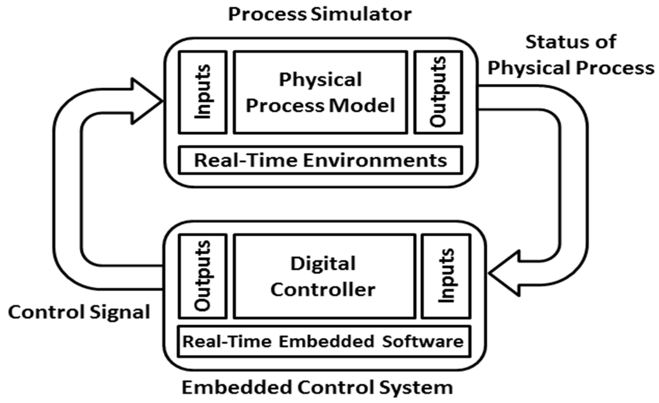
HIL testing has been employed in various domains, such as the aerospace industry [21], automotive applications [23], power electronics and control [24], and marine applications [25]. As discussed, the real-time HIL test-bed introduced in [20] has been employed in this paper. The basic operation of the test bed is that the control software is executed in the microcontroller in real-time, and the controlled system is simulated by a separate desktop computer employing a high-fidelity real-time environment. The outputs of the microcontroller are fed directly as input variables (control signals) to the computer and then the outputs from the computer, which are synthesized from the controlled system, are fed back into the microcontroller, which hosts the control system software, thereby closing the control loop. The general architecture of this facility is illustrated in Figure 3.
The facility consists of two main parts: the first part is the application software (e.g., control algorithms) combined with a task real-time scheduler, which are implemented in an ARM7 microcontroller (LPC2378 processor from NXP© (Eindhoven, The Netherlands). The second is a real-time physical process simulator that is implemented in a desktop PC using the MATLAB© (R2016a, MathWorks, Natick, MA, USA) and Simulink©/Simulink© real-time (R2016a, MathWorks, Natick, MA, USA) software tools. Communication of input/output signals between the PC and embedded system is enabled via a point-to-point Ethernet crossover connection as shown in Figure 4, and a full-duplex data transfer rate of 100 Mbps is achievable. This in effect reduces the latency of data transfers to negligible levels and allows for high-speed sampling rates and high capacity payload transfers of multiple simulation signals simultaneously between the ARM7 microcontroller and the computer.
The user datagram protocol (UDP) is used as a communication protocol and implemented on both sides of the test-bed. UDP is a simple best-effort transport protocol used in most of the delay-sensitive real-time applications; over very short distances (in laboratory conditions), the packet error rate is again negligible. The microcontroller was connected to the computer through a full duplex dedicated link using Ethernet crossover RJ-45 cable, this cable eliminated the need of a network switch to route the data to the PC. This simple setup guaranteed real-time communications since there were no other devices connected to the network, and both microcontroller and computer do not need to wait to send data over the bus. Virtual analog and digital signals are accessed through a simple driver on the embedded platform, and a custom component block within Simulink© (R2016a, MathWorks, Natick, MA, USA).
4.2. Experiment Design
Several experiments lasting 150 s each were performed to examine the behavior of the adaptive MPC controller, verify its tracking performance, and illustrate the performance of various features of the proposed design. The controlled system was represented in Simulink© (R2016a, MathWorks, Natick, MA, USA) by a second-order transfer function of the type shown in Equation (1). The parameters of the controlled system (the gain K, natural frequency ωn, damping ratio ζ, and delay θ) were configured to change between an initial set of values at the start of the experiment to a second set of values at the end. After 60 s of elapsed time, the parameters start to simultaneously ‘drift’ towards the new set of values over the course of approximately 30 s. The initial and final sets of values are shown in Table 1, and the corresponding initial and final discrete transfer functions for a sampling time of 0.1 s are given as Equations (32) and (33) respectively. Two experiments were carried out in these conditions, one with the actuator unconstrained and the other with constraints in place. When constraints were enabled, the process actuator was constrained to lie between 0 and 100% in terms of the amplitude, and ±10% per sample in terms of the slew rate (rate of change of amplitude).
The controller discussed in Section 3 was implemented as three periodic software tasks in the Embedded C language, and hosted on the target hardware. The first task was an input/output task that performed the sampling and actuation processes of the control loop, the second task carried out the model identification activities, and the third task the MPC control. The deadline and period of these tasks have been set to 200 ms. An earliest-deadline first (EDF) task scheduler was employed to schedule the tasks in real-time on the embedded platform. Every 15 s during the simulations, the setpoint was toggled between the values of 10 and 90 in order to ensure the activation of controls was adequately rich in order to activate constraints. A reference trajectory polynomial P(z) = 1 − 0.95 z−1 was employed, generating a first-order response with a (roughly) two second time constant, a reasonable and typical choice for process control applications [1]. The condition number c = 500 was employed to set the move suppression coefficient, again a reasonable and typical choice for process control applications [7]. An extended B polynomial having 10 coefficients was employed to cover the expected range of input delay. During each simulation, Gaussian noise with variance 0.005 was added to the process output. A prediction horizon of 30 samples was employed in each experiment (see, for example, [2,8]). A forgetting factor of 0.99 was employed to enable adaptive identification, see e.g., [4] for justification of this choice. For initialisation purposes, a small step (of amplitude two) was applied for the first 5 s of the simulation. The results obtained are presented in the next section.
4.3. Experimental Results
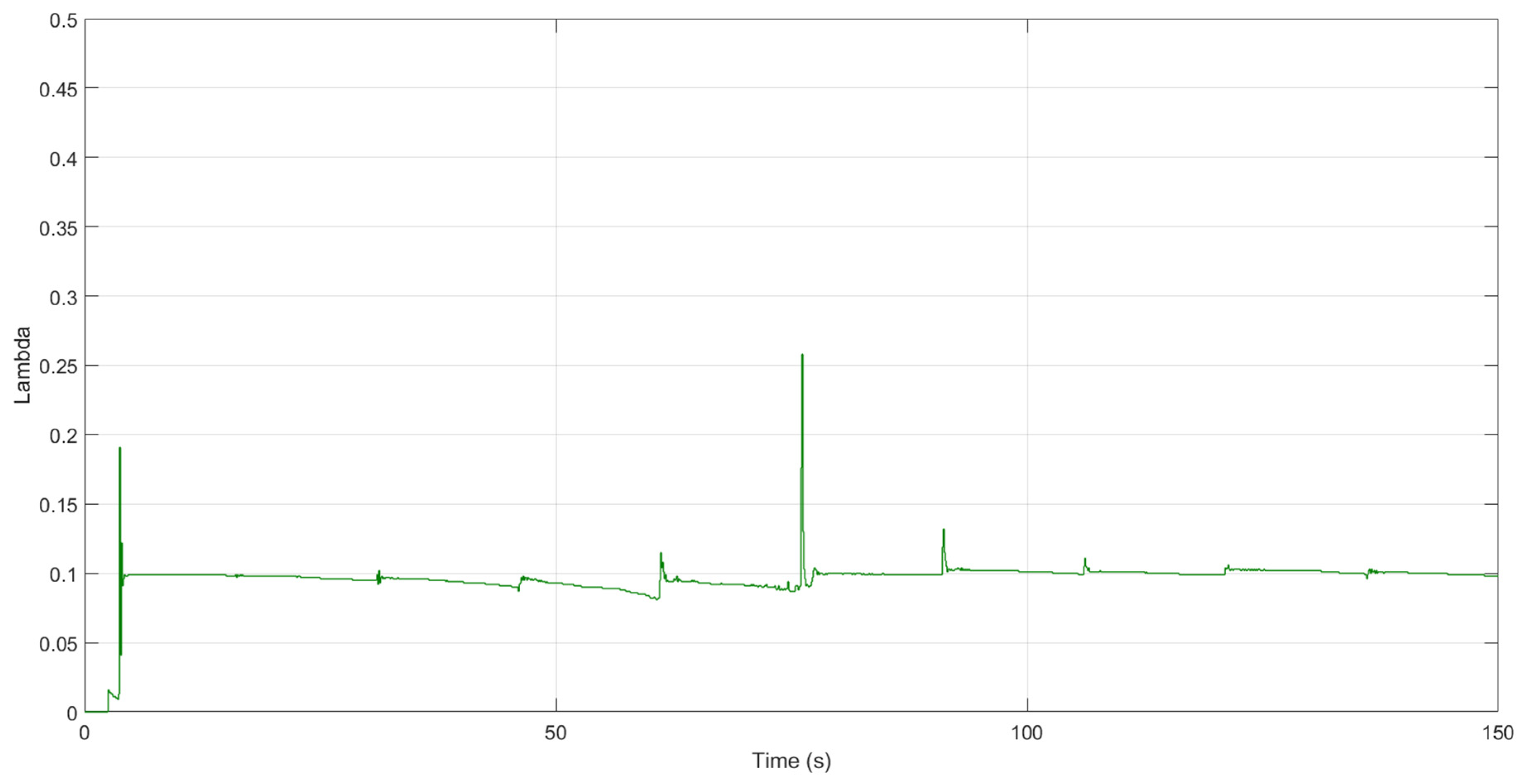
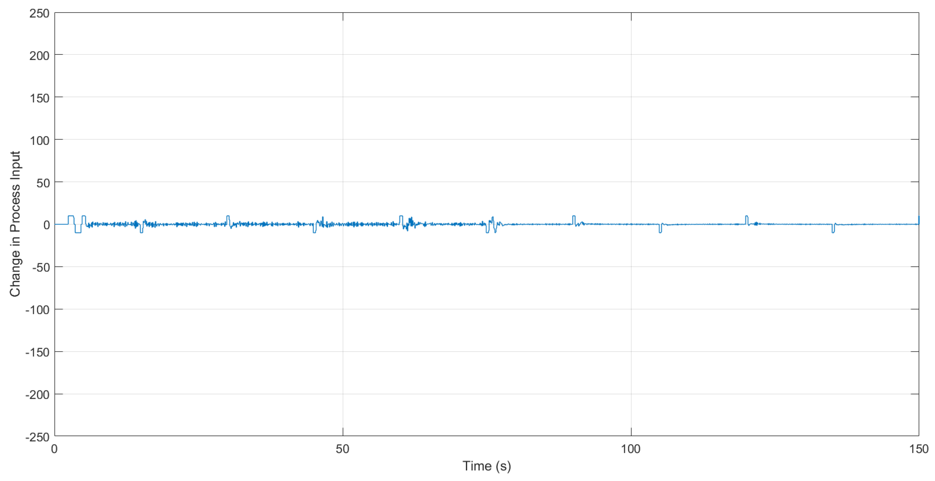
The obtained tracking performance, the control input, the rate-of-change of control input, and the evolution of the move suppression coefficient during the course of the first (unconstrained) experiment are as shown in Figure 5, Figure 6, Figure 7 and Figure 8, respectively. The obtained tracking performance, the control input, the rate-of-change of control input, and the evolution of the move suppression coefficient during the course of the second (constrained) experiment are as shown in Figure 9, Figure 10, Figure 11 and Figure 12, respectively. During the course of the first experiment, after an initial period of convergence (approx. 10 s), the MPC implementation was able to track the process without a problem, giving a response consistent with that of the design specification. During initialization, the process output peaked at a value of 130.8. Following the start of the change in process parameters after 60 s, although there was some impact on the output with a slight decaying oscillation being present, the closed-loop response retained performance from 90 s onwards. The control signal achieved a maximum of 145.1 and a minimum of −118.7 during the experiment, with the largest and smallest applied controls occurring during the initial transient phase. The rate-of-change of applied controls was also at its largest during initialization with a maximum of 238.7 and a minimum of −228.0, but values of the order of 50 occurred during transient phases for the duration of the experiment. The move suppression co-efficient could be seen to quickly tune itself to the characteristics of the identified process and current controller configuration in order to achieve the desired numerical conditioning/robustness. During the period of process parameter drift, it was interesting to observe that, although some chattering on the applied control is evident, this was kept to a bounded level due to the conditioning of the controller. In addition, the move suppression coefficient was transiently increased for a short time around the 75 s mark when a setpoint change occurred during the parameter transient. This additional input excitation clearly encouraged changes to the estimated parameters, and move suppression was increased to compensate as the controller lost conditioning. As the estimates converged around the 85 s mark, the move suppression co-efficient converged to a value slightly above its previous value.
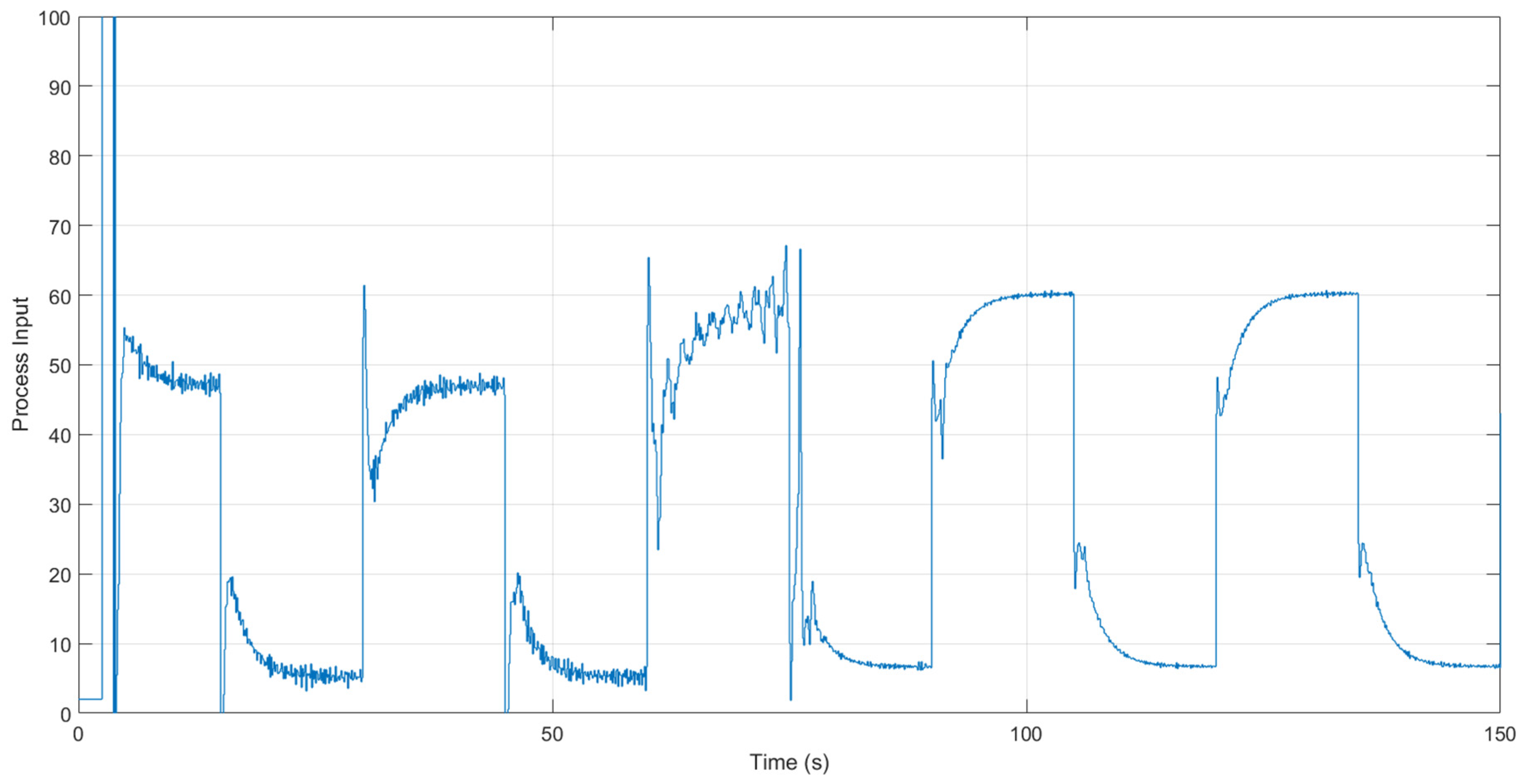
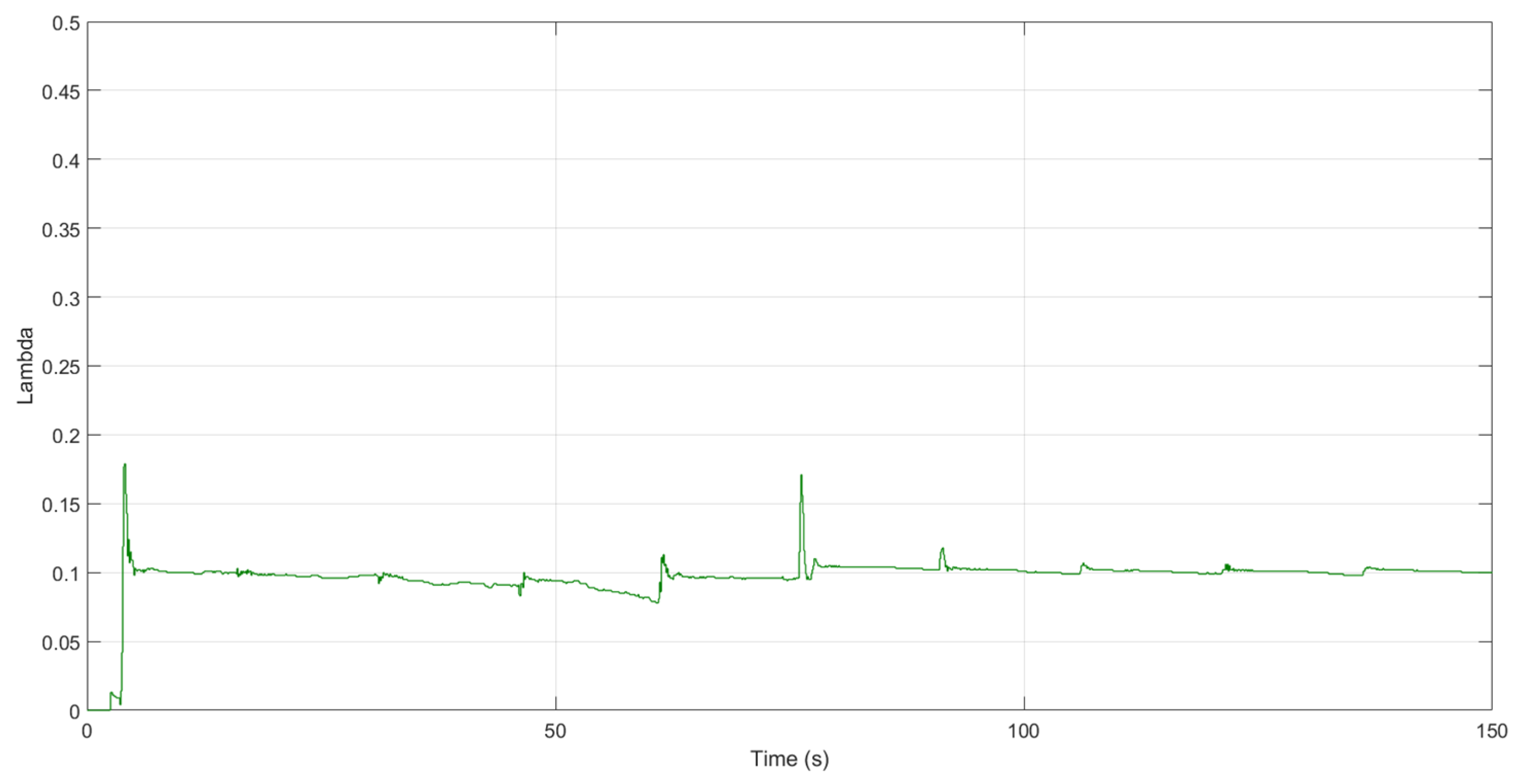
During the course of the second experiment, there was again an initial period of convergence (approx. 10 s), after which the MPC implementation was able to track the process without a problem, giving a response consistent with that of the design specification within the bounds of the input constraints. During initialization, the process output peaked at a much lower value of 96.3. Following the start of the change in process parameters after 60 s, although again there was some impact on the output with a slight decaying oscillation being present, the oscillation was smaller in the constrained case (due to the input chattering being suppressed by the constraints themselves). The closed-loop response again retained performance from 90 s onwards. As expected, the control signal achieved a maximum of 100.0 and a minimum of 0.0 during the experiment, with the largest and smallest applied controls occurring during the initial transient phase. The rate-of-change of applied controls was also as expected, with a maximum of 10.0 and a minimum of −10.0 for the duration of the experiment. The move suppression co-efficient could again be seen to quickly tune itself to the characteristics of the identified process and current controller configuration in order to achieve the desired numerical conditioning/robustness, and follows a similar evolution to the unconstrained case. However, during the period of process parameter drift, it was interesting to observe that the chattering on the applied control was again present but was kept bound at a smaller level than the unconstrained case, due to the constraints as well as the conditioning of the controller. The move suppression coefficient was again transiently increased for a short time around the 75 s mark, but as the constraints acted to additionally limit the input excitation when the setpoint change occurred, the magnitude of the move suppression increase was less than the previous case. As the estimates converged around the 85 s mark, the move suppression co-efficient again converged to a value slightly above its previous.
Over the course of both experiments, the combined execution times of the tasks for both identification and MPC control never exceeded 51 ms. Of this overhead, approximately one-third of the computation time was required for identification and the rest for control. This was a small overhead for a resource-constrained embedded platform and gave a good indication of the efficiency of the proposed approach. In terms of scalability, it is worth noting that the RLS algorithm scales quadratically in the number of estimated parameters, while the MPC control scales linearly in the length of the prediction horizon. Therefore, the identification of a larger model with more parameters is likely to have a larger relative impact on computation overhead when compared to increasing the length of the prediction horizon.
5. Conclusions
In this paper, it has been argued that, although MPC has a significant drawback in terms of the potentially large computational burden in adaptive and constrained situations, it is still possible to create a computationally efficient self-tuning/adaptive MPC scheme for simple industrial plant on a small microcontroller platform. A control approach that handles rate and amplitude constraints on the plant input by employing a short (2-step) control horizon and by automatically tuning the move suppression (regularization) parameter to achieve well-conditioned and robust control has been developed. Preliminary hardware-in-the-loop (HIL) test results indicate that the resulting scheme performs well, robustly tracks changes in the process parameters whilst respecting the input constraints, and has a low implementation overhead. Future work will consider the extension of the proposed approach to longer control horizons, incorporating elements of the extension to the basic Hildreth algorithm to accelerate convergence [6].
Author Contributions
Michael Short developed the MPC control algorithm described in the paper, created the code for its implementation, and prepared the manuscript. Fathi Abugchem ported the code to the microcontroller platform, performed the experimentation, and collated the results.
Conflicts of Interest
The authors declare no conflict of interest.
References
- Camacho, E.F.; Bordons, C. Model Predictive Control, 2nd ed.; Springer-Verlag: Berlin, Germany, 2003. [Google Scholar]
- Morari, M.; Lee, J.H. Model predictive control: past, present and future. Comput. Chem. Eng. 1999, 23, 667–682. [Google Scholar] [CrossRef]
- Clarke, D.W.; Mohtadi, C.; Tuffs, P.S. Generalized Predictive Control—Parts I & II. Automatica 1997, 23, 137–160. [Google Scholar]
- Astrom, K.J.; Wittenmark, B. Adaptive Control, 2nd ed.; Addison-Wesley Publishing: Boston, MA, USA, 1995. [Google Scholar]
- Saffer, D.R., II; Doyle, F.J., III. Analysis of linear programming in model predictive control. Comput. Chem. Eng. 2004, 28, 2749–2763. [Google Scholar] [CrossRef]
- Short, M. A simplified approach to Multivariable Model Predictive Control. Int. J. Eng. Technol. Innov. 2015, 5, 19–32. [Google Scholar]
- Short, M. Move Suppression Calculations for Well-Conditioned MPC. ISA Trans. 2017, 67, 371–381. [Google Scholar] [CrossRef] [PubMed]
- Garriga, J.L.; Soroush, M. Model Predictive Control Tuning Methods: A Review. Ind. Eng. Chemisty Res. 2010, 49, 3505–3515. [Google Scholar] [CrossRef]
- Marjanovik, O.; Lennox, B.; Goulding, P.; Sandoz, D. Minimising conservatism in infinite-horizon LQR control. Syst. Control Lett. 2002, 46, 271–279. [Google Scholar] [CrossRef]
- Mare, J.B.; De Dona, J.A. Solution of the input-constrained LQR problem using dynamic programming. Syst. Control Lett. 2006, 56, 342–348. [Google Scholar] [CrossRef]
- Pannocchi, G.; Laachi, N.; Rawlings, J.B. A Fast, Easily Tuned SISO Model Predictive Controller. In Proceedings of the 7th IFAC Symposium on Dynamics and Control of Process Systems 2004 (DYCOPS -7), Cambridge, MA, USA, 5–7 July 2014; pp. 907–912. [Google Scholar]
- Mare, J.B.; De Dona, J.A. Elucidation of the state-space regions wherein model predictive control and anti-windup strategies achieve identical control policies. In Proceedings of the American Control Conference, Chicago, IL, USA, 28–30 June 2000; pp. 1924–1928. [Google Scholar]
- Short, M. Real-Time Infinite Horizon Adaptive/Predictive Control for Smart Home HVAC Applications. In Proceedings of the 17th IEEE International Conference on Emerging Technology Factory Automation, Krakow, Poland, 17–21 September 2012. [Google Scholar]
- Camacho, E.F. Constrained Generalized Predictive Control. IEEE Trans. Autom. Control 1993, 38, 327–332. [Google Scholar] [CrossRef]
- Tsang, T.T.C.; Clarke, D.W. Generalized predictive control with input constraints. IEE Proc. Part D Control Theory Appl. 1988, 135, 451–460. [Google Scholar] [CrossRef]
- Kheriji Abbes, A.; Bouani, F.; Ksouri, M. A Microcontroller Implementation of Constrained Model Predictive Control. World Acad. Sci. Eng. Technol. 2011, 5, 655–662. [Google Scholar]
- Huyck, B.; Brabanter, J.D.; Moor, B.D.; Van Impe, J.F.; Logist, F. Online model predictive control of industrial processes using low-level control hardware: A pilot-scale distillation column case study. Control Eng. Pract. 2014, 28, 34–48. [Google Scholar] [CrossRef] [Green Version]
- Ljung, L. System Identification: Theory for the User; Prentice Hall: Upper Saddle River, NJ, USA, 1997. [Google Scholar]
- Tuffs, P.S.; Clarke, D.W. Self-tuning control of offset: a unified approach. IEE Proc. 1985, 132, 100–110. [Google Scholar] [CrossRef]
- Abugchem, F.; Short, M.; Xu, D. A Test Facility for Experimental HIL Analysis of Industrial Embedded Control Systems. In Proceedings of the 17th IEEE International Conference on Emerging Technologies Factory Automation (ETFA), Krakow, Poland, 17–21 September 2012. [Google Scholar]
- Sun, Y.P. The Development of a Hardware-in-the-Loop Simulation System for Unmanned Aerial Vehicle Autopilot Design Using LabVIEW. In Practical Applications and Solutions Using LabVIEW™ Software; Dr., Silviu, F., Ed.; InTech: Vienna, Austria, 2011. [Google Scholar]
- Bacic, M. On hardware-in-the-loop simulation. In Proceedings of the 44th IEEE Conference on Decision and Control and European Control Conference, Seville, Spain, 12–15 December 2005; pp. 3194–3198. [Google Scholar]
- Short, M.; Pont, M.; Fang, J. Assessment of performance and dependability in embedded control systems: methodology and case study. Control Eng. Pract. 2008, 16, 1293–1307. [Google Scholar] [CrossRef]
- Lu, B.; Wu, X.; Figueroa, H.; Monti, A. A Low-Cost Real-Time Hardware-in-the-Loop Testing Approach of Power Electronics Controls. IEEE Trans. Ind. Electron. 2007, 54, 919–931. [Google Scholar] [CrossRef]
- Skjetne, R.; Egeland, O. Hardware-in-the-loop testing of marine control system. Model. Ident. Control 2006, 27, 239–258. [Google Scholar] [CrossRef]
Figure 1.
Adaptive model predictive control (MPC) Control Structure.
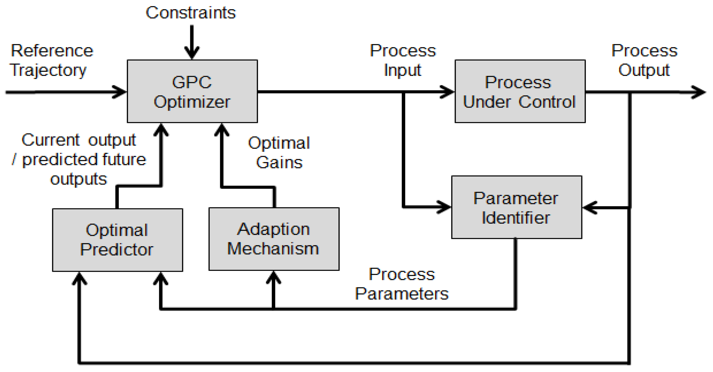
Figure 2.
Principle of hardware-in-the-loop (HIL) testing.

Figure 3.
General architecture of the HIL testing facility.

Figure 4.
Hardware components of the HIL testing facility.
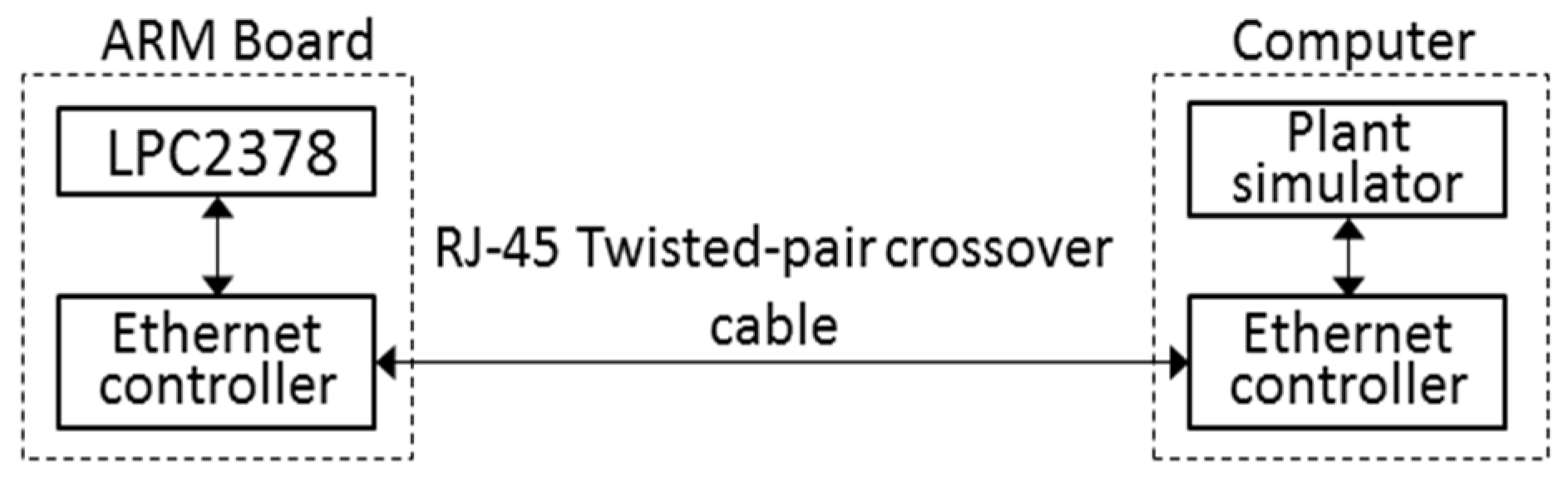
Figure 5.
Tracking performance of the controller in the unconstrained case. Red: process output; black: setpoint.
Figure 5.
Tracking performance of the controller in the unconstrained case. Red: process output; black: setpoint.
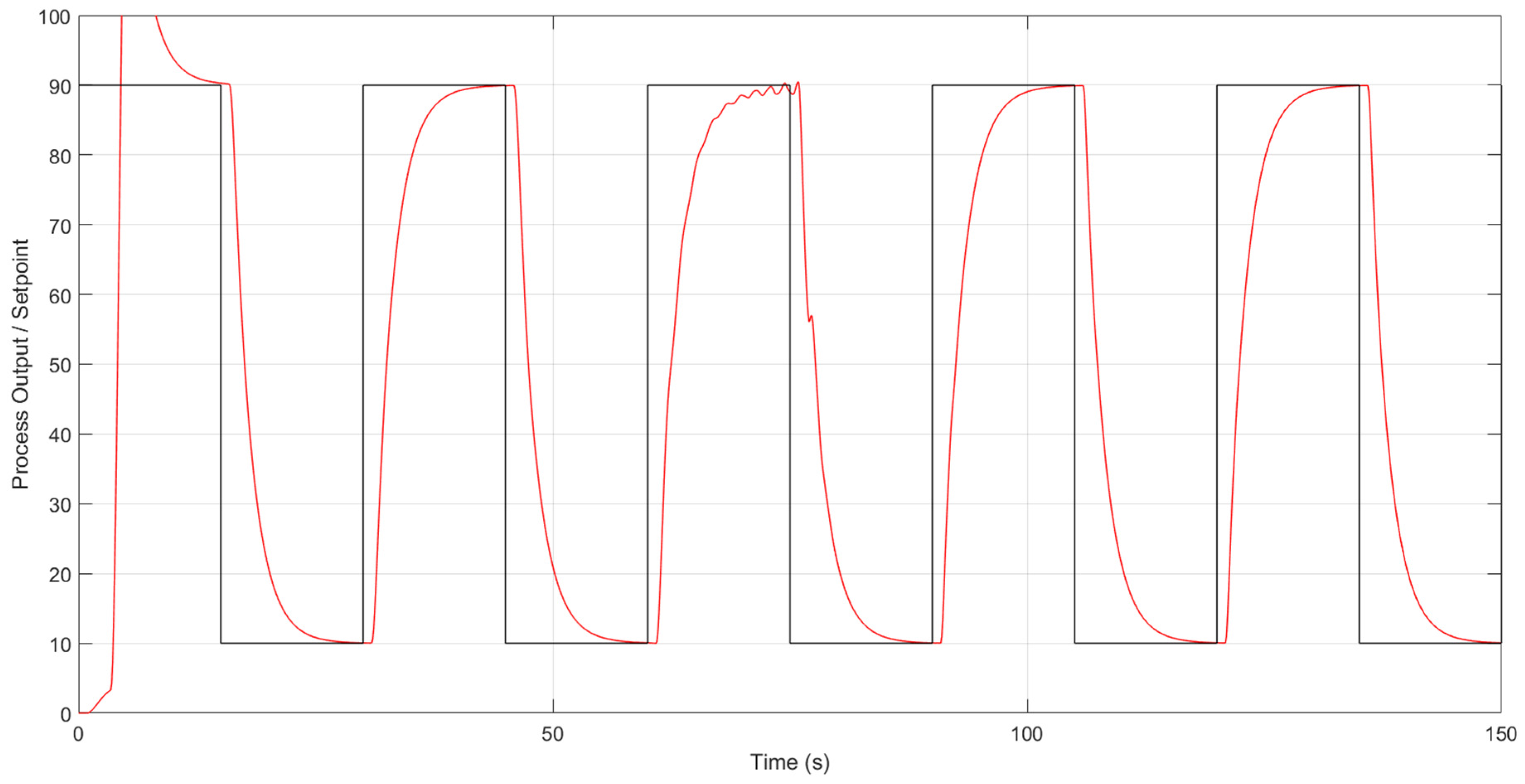
Figure 6.
Applied controls (process input) in the unconstrained case.

Figure 7.
Rate-of-change of applied controls (process input) in the unconstrained case.
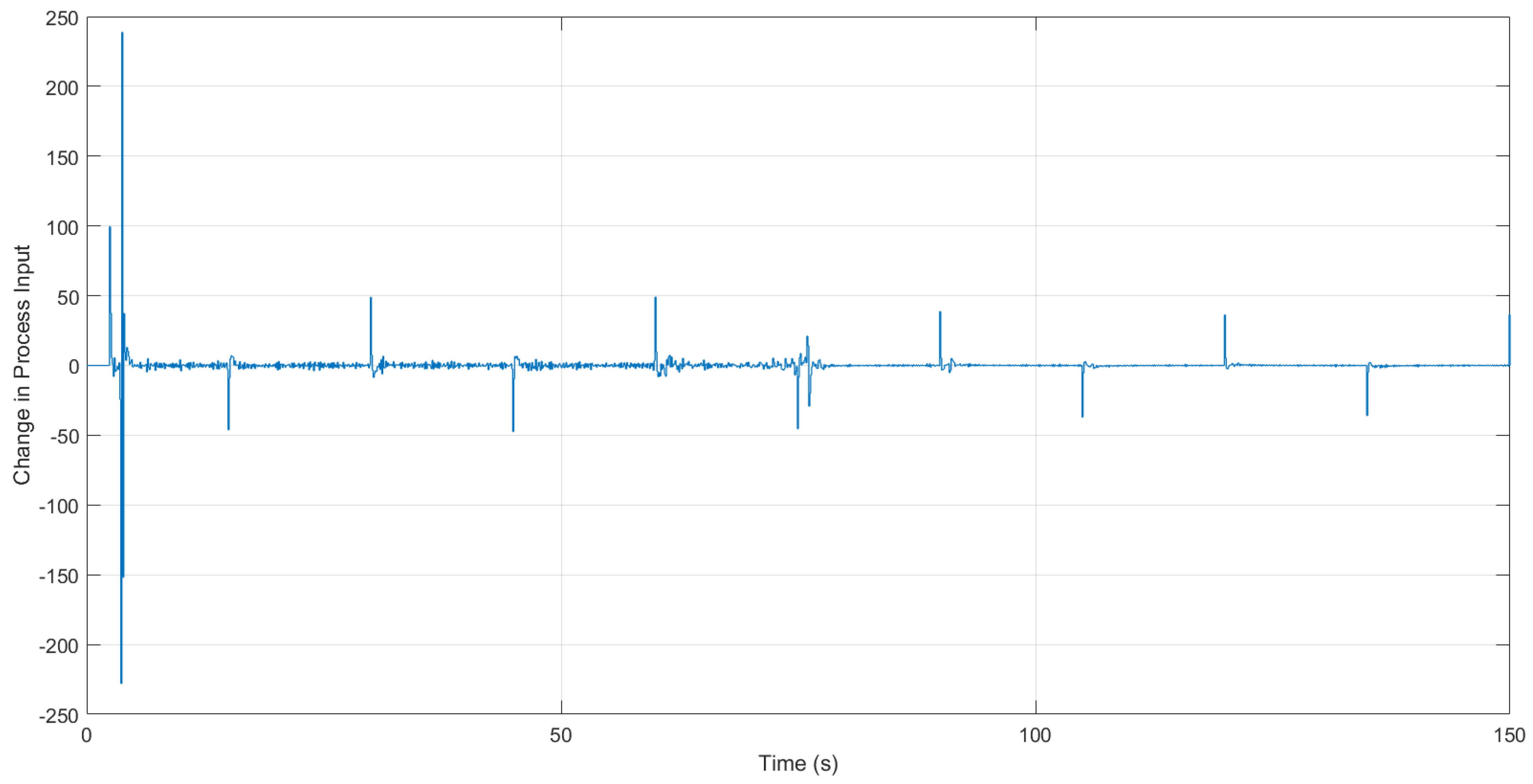
Figure 8.
Evolution of the move suppression coefficient in the unconstrained case.

Figure 9.
Tracking performance of the controller in the constrained case. Red: process output; black: setpoint.
Figure 9.
Tracking performance of the controller in the constrained case. Red: process output; black: setpoint.
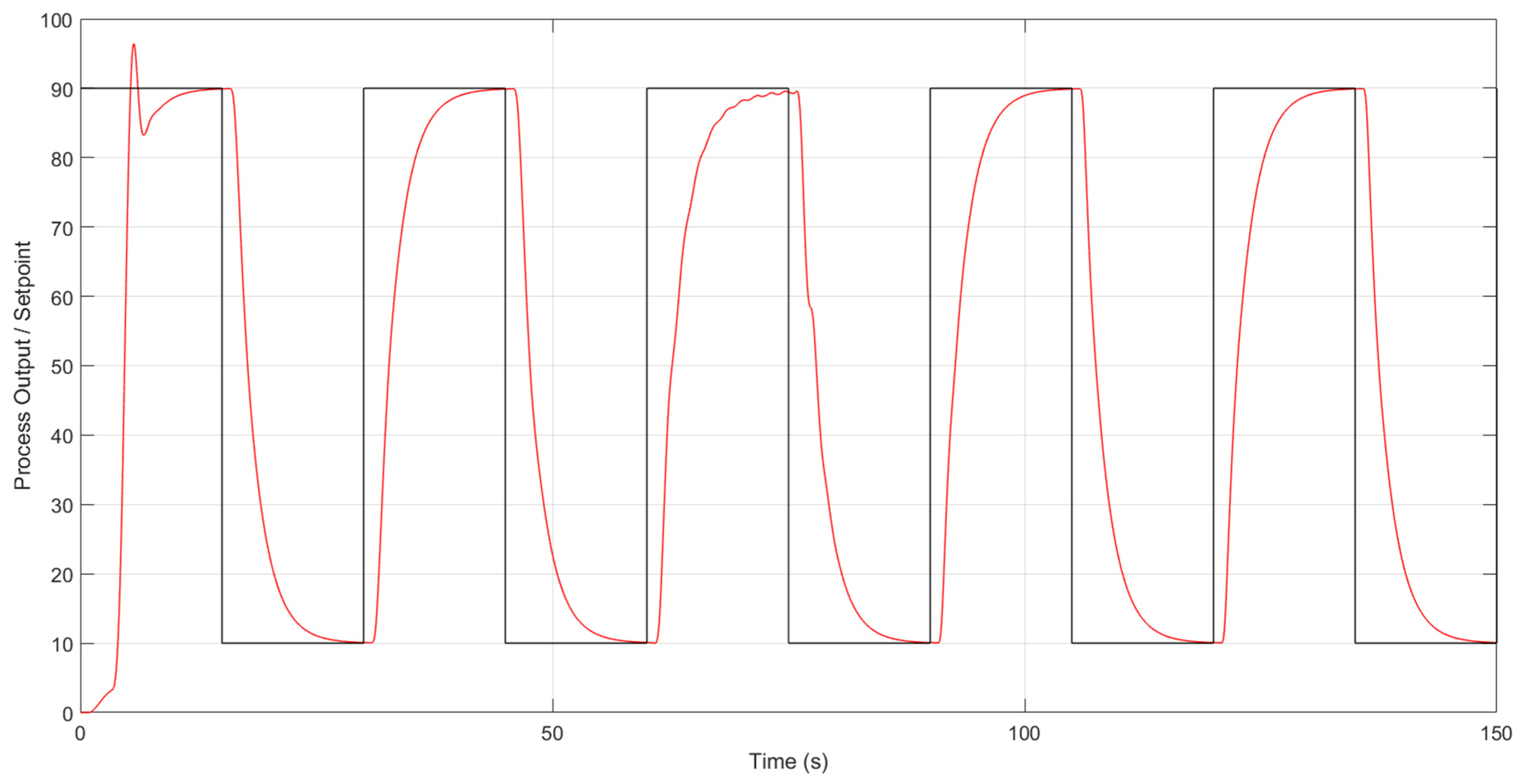
Figure 10.
Applied controls (process input) in the constrained case.
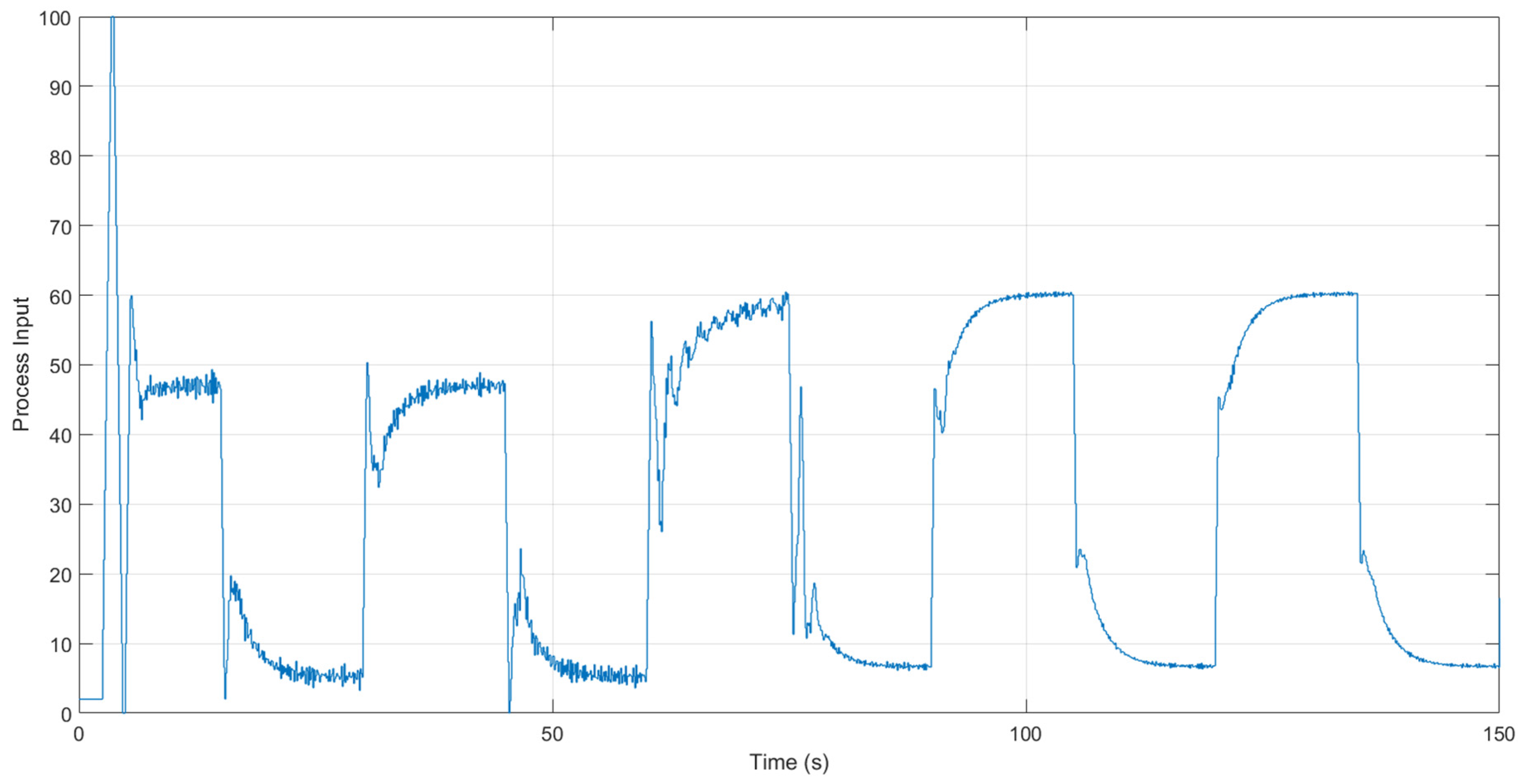
Figure 11.
Rate-of-change of applied controls (process input) in the constrained case.

Figure 12.
Evolution of the move suppression coefficient in the unconstrained case.


Table 1.
Parameters and configuration of the time-varying system.
| Parameter | Initial Value | Final Value |
|---|---|---|
| K | 2 | 1.5 |
| ωn | 2 | 1.75 |
| ζ | 0.75 | 1.25 |
| θ | 1 | 0.5 |
© 2017 by the authors. Licensee MDPI, Basel, Switzerland. This article is an open access article distributed under the terms and conditions of the Creative Commons Attribution (CC BY) license (http://creativecommons.org/licenses/by/4.0/).
Share and Cite
MDPI and ACS Style
Short, M.; Abugchem, F. A Microcontroller-Based Adaptive Model Predictive Control Platform for Process Control Applications. Electronics 2017, 6, 88. https://doi.org/10.3390/electronics6040088
AMA Style
Short M, Abugchem F. A Microcontroller-Based Adaptive Model Predictive Control Platform for Process Control Applications. Electronics. 2017; 6(4):88. https://doi.org/10.3390/electronics6040088
Chicago/Turabian StyleShort, Michael, and Fathi Abugchem. 2017. "A Microcontroller-Based Adaptive Model Predictive Control Platform for Process Control Applications" Electronics 6, no. 4: 88. https://doi.org/10.3390/electronics6040088
Note that from the first issue of 2016, this journal uses article numbers instead of page numbers. See further details here.