Robust Offset-Free Speed Tracking Controller of Permanent Magnet Synchronous Generator for Wind Power Generation Applications


1
Department of Creative Convergence Engineering, Hanbat National University, Daejeon 341-58, Korea
2
Department of Electrical and Computer Engineering, Ajou University, Suwon 443-749, Korea
*
Author to whom correspondence should be addressed.
Electronics 2018, 7(4), 48; https://doi.org/10.3390/electronics7040048
Submission received: 16 March 2018
/
Revised: 2 April 2018
/
Accepted: 3 April 2018
/
Published: 4 April 2018
(This article belongs to the Special Issue Renewable Electric Energy Systems)
Abstract
:This article presents a robust speed tracking algorithm for a permanent magnet synchronous generator utilized for wind power generation systems, considering the machine parameter and load uncertainties. There are two major contributions: (a) a disturbance observer is designed to exponentially estimate disturbances from the model-plant mismatches and severe load torque variations, and (b) it is included in a nonlinear cascade-type proportional speed tracking controller to establish the performance recovery and offset-free properties without the use of tracking error integrators. A simulation result numerically verifies the effectiveness of the proposed technique, where the PowerSIM software emulates a wind power generation system.
1. Introduction
Permanent magnet synchronous machines (PMSMs) have been widely adopted for wind power generation systems because of their high efficiency and control performance [1,2,3,4,5,6], and the PMSM controller plays the pivotal role of securing high reliability for wind power generation systems. In particular, the speed tracking performance must be maximized for a satisfactory maximum power point tracking (MPPT) control [7].
The PMSM current and voltage behaviors can be described as vectors determined by coordinate systems. Because these current and voltage vectors given in the d-q rotational coordinate system represent their DC-components, the current tracking problem can easily be solved through the use of a simple proportional-integral (PI) regulator. This result certainly aids solving the speed tracking problem under the cascade control strategy, where the outer-loop PI speed regulator automatically computes the desired q-axis current reference for the inner-loop PI current regulator [8]. This PI cascade speed controller has been widely used in several industrial applications because of its simplicity. The PI gains determine the closed-loop performance and were designed to meet the specification described in the frequency domain under a given operating condition. Thus, an additional gain-scheduling algorithm as in [9] should be embedded in the control algorithm to achieve a satisfactory closed-loop performance under several operating conditions. A feed-forward compensation technique was proposed to eliminate disturbances by the back electromotive force (EMF) effect, which is interpreted as the feedback-linearization (FL) technique in the control theoretical perspective [10,11]. The corresponding PI gains were systematically designed using the PMSM true parameter values to transform the closed-loop behavior into a desired low-pass filter (LPF) dynamics. However, the parameter dependency still requires the use of an additional parameter identification (on/off-line) or gain scheduling algorithms.
A model predictive, an observer, and a sliding mode control (SMC) based techniques have been applied to both inner and outer-loops. The model predictive control (MPC) technique optimizes the cost function of tracking errors by predicting the states, one or two-steps ahead, utilizing PMSM parameters [12,13]. The optimization procedure was conducted through an exhaustive search method for each control period, and the offset-free property was obtained by adopting tracking error integrators. The disturbance observer (DOB) was designed to simultaneously estimate both state and disturbance using the PMSM parameters, combined with a robust stabilizing controller [14]. The active disturbance attenuation property was obtained with a PMSM position estimator based on a high-gain observer depending on PMSM parameters [15]. Sliding mode techniques were utilized to obtain a robust stabilization property, which contains a conservative feed-forward compensation term with a high-gain discontinuous sign-function; it could make the control input infeasible for some transient periods [16,17]. A passivity-based PI speed regulator was recently presented with an adaptive time-delay compensator [6]. However, there was no systematic procedure to adjust the closed-loop speed tracking performance.
Unlike aforementioned literatures depending on the true machine parameters with tracking error integrators, this study systematically designs a proportional-type speed controller by considering nonlinear dynamics with parameter and severe load torque variations emanating from the wind turbine and wind velocity. The resulting controller is in the form of a cascade structure. Both inner and outer-loop controllers are derived to simultaneously stabilize current and speed tracking error dynamics, whereas feedbacks simply proportionate tracking errors with the dynamic disturbance compensation terms generated by the DOBs. The first contribution is to design exponential convergent DOBs for the inner and outer-loops using only nominal PMSM parameters. The second one is to incorporate resulting DOBs into a nonlinear proportional-type speed tracking controller. These two features could further effect the control algorithm simplification by eliminating the use of tracking error integrators as well as anti-windup algorithms. The effectiveness of the proposed controller is demonstrated by conducting realistic simulations using the PowerSIM (PSIM) software with the dynamic-link library (DLL) block for the controller.
2. Dynamics of Permanent Magnet Synchronous Generator with Wind Turbine in Rotational d-q Axis
In the rotational d-q axis, the speed and current dynamics of the permanent magnet synchronous generator (PMSG) can be described as [18]
where the mechanical parameters B and J represent viscous damping and total inertia, including the rotor and wind turbine, respectively; the mechanical speed and d-q axis current vector function as state-variables; the d-q axis stator voltage vector is used as the control input to be designed later. The state-dependent back-EMF term is defined as with the d-q axis inductance matrix , the pole pair P, and the magnet flux , respectively. The electrical output torque is given by
with the d-q axis inductance difference of , and the load torque emanating from the wind turbine with wind velocity is described as [19]
with , R, , , , and denoting the air density, blade radius, pitch angle, tip-speed ratio, and wind velocity, respectively. The wind turbine power can be approximately written as
where , .
Considering the model-plant mismatches and unexpected severe load torque variations from the wind turbine with the wind velocity, it is reasonable to consider the nominal PMSG dynamics for designing the controller, instead of (1) and (2):
with nominal parameters , , , , and , where the nominal electrical output torque and back-EMF term are defined as
and
respectively, and unknown lumped disturbances are represented as and . In the rest of this article, a speed tracking algorithm is designed based on the perturbed PMSG dynamics of (6) and (7).
3. Speed Tracking Algorithm Design
This section devises a speed tracking algorithm to transform the closed-loop speed dynamics into
where and represent the Laplace transforms of the speed and its reference , respectively, and refers to the cut-off frequency used as a design parameter. For the speed-loop, the design parameters are given as and , and the current-loop design parameters correspond to and , which adjusts the speed and current convergent behaviors. Section 3.1 derives the stabilizing q-axis current reference with the closed-loop speed tracking error dynamics, and Section 3.2 constructs the final speed control law using the resulting q-axis current reference and analyzes closed-loop properties.
3.1. Outer-Loop Controller Design
In order to achieve the control objective of (8), consider the target dynamics given by
and define the speed tracking error as , . Then, it follows that
where and , , which can be stabilized by the proposed q-axis current reference given by
with a design parameter of , where the disturbance estimate is defined as
and the state variable satisfies
with a design parameter of . The dynamic system comprising the state equation of (13), and the output equation of (12) is defined as the outer-loop DOB in this study. The closed-loop speed tracking error dynamics can be obtained by combining (10) and (11) as
where , .
3.2. Inner-Loop Controller Design and Closed-Loop Property Analysis
This section derives an inner-loop controller to stabilize the speed and current tracking error dynamics, simultaneously. For this purpose, define the current tracking error as , , with the current reference of , , where the q-axis current reference of comes from (11), which gives the current tracking error dynamics as
with the unknown lumped disturbance , . Then, to stabilize the current tracking error dynamics of (15), the control law for the d-q stator voltage of is proposed as
with design parameters of and , where the disturbance estimate of is defined as
and the state variable satisfies
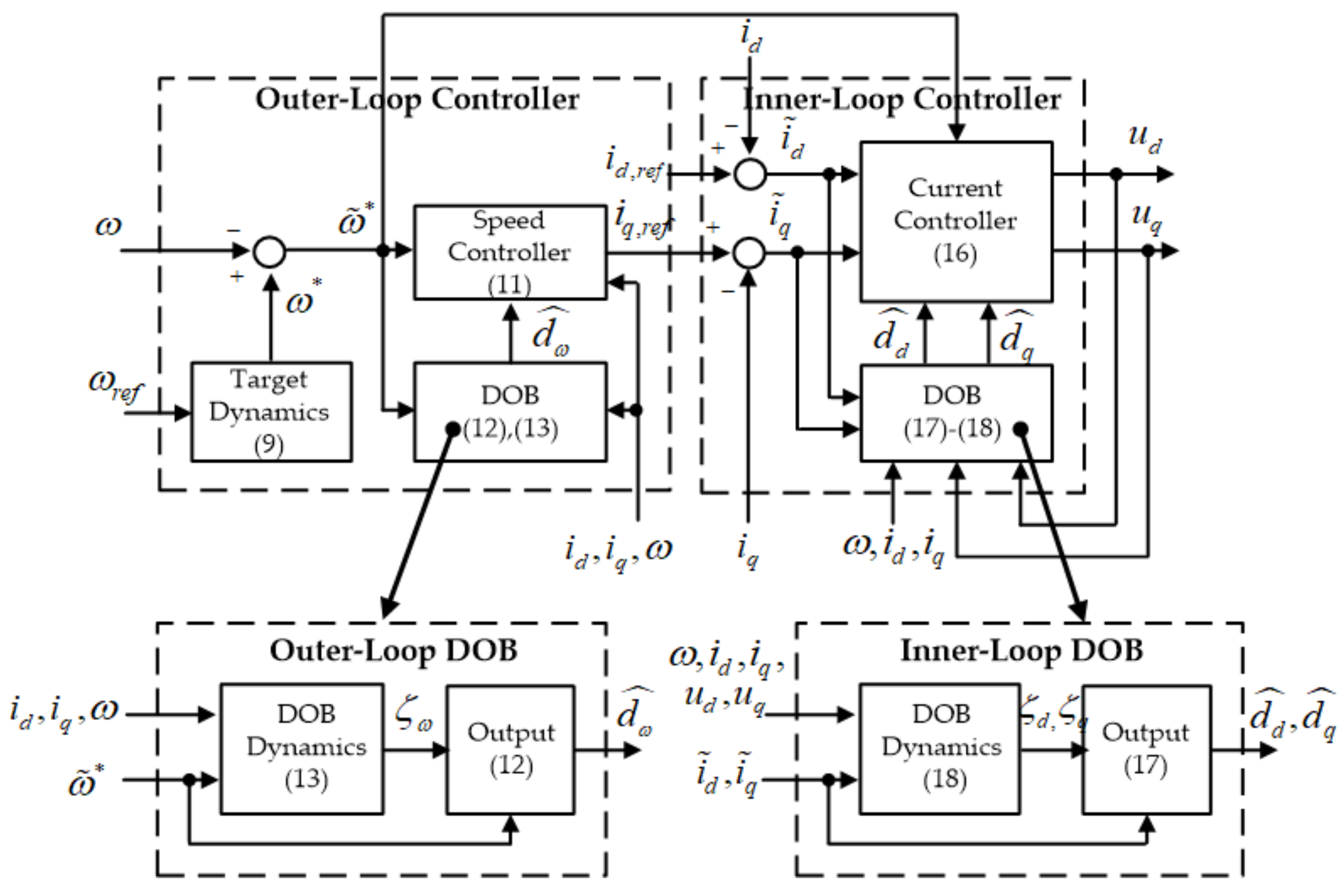
with a design parameter . The dynamic system comprising the state equation of (18) and output equation of (17) is defined as the inner-loop DOB in this study. The proposed controller structure is visualized in Figure 1. The closed-loop current tracking error dynamics can be obtained by combining (15) and (16) as
where , .
Theorem 1 presents the stabilization property of the closed-loop system, and the proof is provided in the Appendix.
Theorem 1.
The analysis result of Theorem 1 implies that the exponential performance recovery property can be established by the proposed controller, as disturbances and exponentially reach their steady-states. In other words, the proposed controller can accomplish the control objective of (8) in an exponential manner. The Appendix proves the statement of Theorem 1 by showing that the closed-loop tracking error trajectories coerce the positive definite function of
to be
for some , , .
Theorem 2 asserts that the closed-loop system guarantees the offset-free property, which is not evident because the proposed controller only feedbacks the tracking error proportional term, as shown in (11) and (16). The outer and inner loop DOBs provide this beneficial property. For details, see Theorem 2 and the Appendix for proof.
4. Simulations
This section numerically verifies the features of the proposed technique, which are rigorously proven by Theorems 1 and 2.
4.1. Wind Power System Configuration
The PSIM software emulates the wind power generation system, whereas the DLL block, created using by the C-language, implements the control algorithms. The three-phase inverter was introduced to synthesize the stator voltage command generated by the control law. The DC-link voltage was regulated to V by the grid-side converter. The pulse-wide modulation (PWM) and control periods were set to be synchronized to ms. The PMSG true parameters were given by
and nominal PMSM parameters were picked as
which were utilized for controller implementations. Note that the parameter J represent the total inertia, including the PMSG and wind turbine. The wind turbine block provided in the PSIM software was used, where the nominal output power, inertia, base wind speed, base rotational speed, and initial rotational speed were set to 10-kW, , , 50 rpm, and 10 rpm, respectively. The wind was randomly generated according to the Weibull distribution-based wind model [20] presented in Figure 2. Figure 3 shows the wind power generation system implementation including the speed controller.
4.2. Controller Configuration
The FL controller was used for comparison and is given by
with the q-axis current reference obtained from
where , , and and denote the cut-off frequencies of the current and speed loops, respectively. The closed-loop dynamics driven by the FL controller can be approximately given as
for a slowly time-varying load torque of , where represents the Laplace transform , . Note that the d-axis current reference of was set to zero for the maximum torque per ampere (MTPA) operation because the PMSG used in this simulation is seemingly that of a surfaced-type, i.e., .
The cut-off frequencies used for both controllers were set to Hz and Hz for and . For the proposed controller, and the control and DOB gains were tuned as and , .
4.3. Simulation Scenario and Evaluation Metric
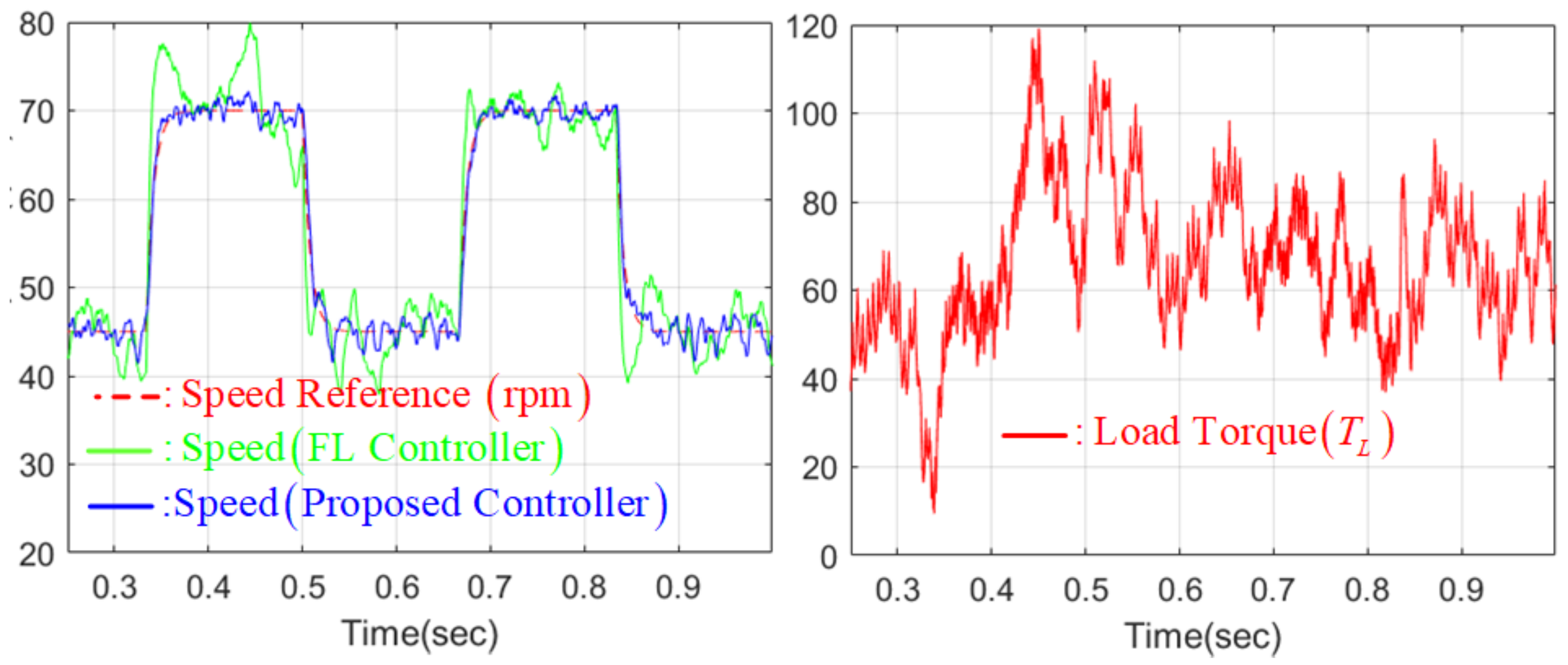
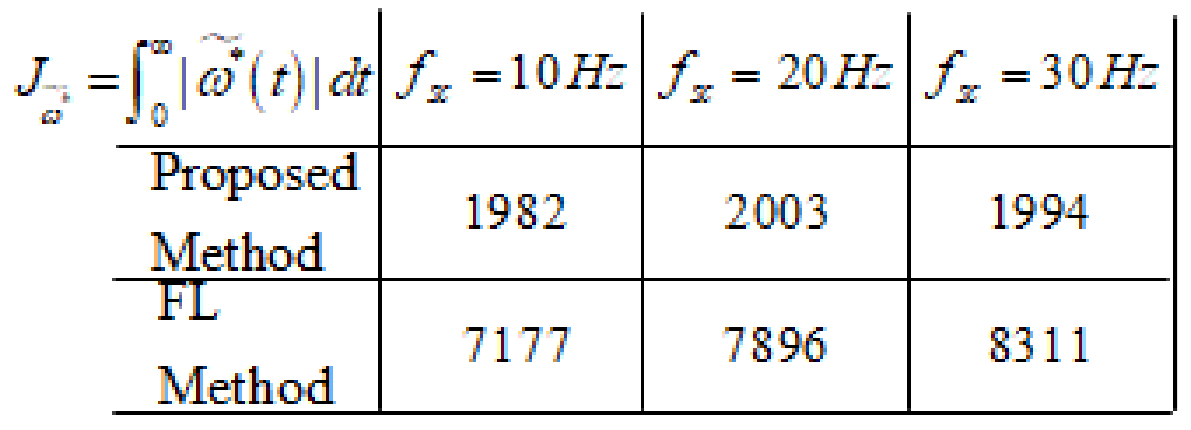
The numerical evaluations were performed under the periodical time-varying speed reference which is given in a pulse wave form at 3 Hz, whose minimum and maximum values correspond to 45 and 70 rpm, respectively. For quantitative evaluations, a metric function of was introduced as
where and denote the target speed trajectory of (9) and the closed-loop speed trajectory, respectively.
4.4. Numerical Verification Results
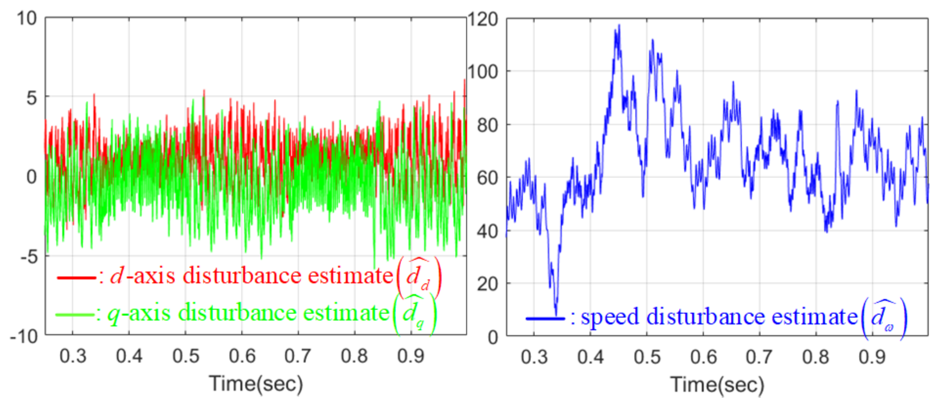
The speed tracking performance comparison result with the load torque behavior is depicted in Figure 4, whereas Figure 5 presents the d-q axis current behaviors. In particular, Figure 4 shows that the proposed method robustly drives the PMSG speed to its reference while maintaining the tracking performance at the desired level in the presence of model-plant mismatches and severe load torque variations. The disturbance estimate from DOBs are presented in Figure 6.
At this stage, all design parameters, except for the cut-off frequency of , were retained as those used under previous simulation settings. Speed tracking performance changes for various cut-off frequencies were observed as Hz, which were applied to both controllers. As can be seen from Figure 7, the proposed technique successfully and precisely assigned the desired speed tracking performance to the closed-loop system using the fixed design parameter. However, the FL controller failed, which is regarded a practical benefit of this study.
Figure 8 summarizes the resulting evaluation values coming from the metric function of , which clearly turns out that the proposed technique considerably enhances the closed-loop robustness by keeping the metric values similar for different cut-off frequencies.
These numerical results clearly confirm the useful closed-loop properties proven by Theorems 1 and 2, the performance recovery and offset-free properties, and the use of the fixed design parameter. It was observed that the proposed method successfully keeps the closed-loop performance desirable under severe load torque variations caused by wind velocity.
5. Conclusions
This paper proposes the use of a proportional-type nonlinear stabilizing speed tracking controller incorporating DOBs, instead of tracking error integrators. The proposed controller and DOBs were designed based on the nominal PMSG dynamics so as to remove the parameter dependency. The beneficial closed-loop properties rigorously proven in this study were numerically verified by performing a realistic simulation. Theoretical and numerical evidences indicate that the proposed technique qualifies as a potential solution to achieve a satisfactory MPPT operation. This study does not provide any systematical way to tune the design parameters for an acceptable closed-loop performance, which will be addressed in a future study. Moreover, it is also desirable for a future study to experimentally verify the power generation efficiency improvement under the MPPT operation including the proposed speed tracking algorithm.
Acknowledgments
This research was supported by Basic Science Research Program through the National Research Foundation of Korea (NRF) funded by the Ministry of Education(2017R1C1B5074256) and was supported by the National Research Foundation of Korea (NRF) grant funded by the Korea government (MSIT) (No. 2016R1A2B4010636).
Author Contributions
Seok-Kyoon Kim surveyed the backgrounds of this research, designed the whole control and estimation algorithms, and performed the simulations so as to show the novelties of the proposed technique. Kyo-Beum Lee supervised and financially supported this study.
Conflicts of Interest
The authors declare no conflict of interest.
Appendix A
This section gives the proofs of Theorems 1 and 2. First, the proof of Theorem 1 is given by:
Proof.
The lumped disturbances, and , in (10) and (15) satisfy
and the combination of DOB outputs of (12), (17), and state equations of (13), (18) yield that
which gives
using the equations of (A1) and (A2). At this point, consider the positive definite function defined in (21) as
which gives the time-derivative of using the trajectories of (14), (19) and (A3) as
The application of Young’s inequality , , to indefinite terms in the inequality of (A5) leads to
Eventually, the constants and render as
which results in the strict passivity of the input-output mapping of (20). □
Second, the proof of Theorem 2 is given by:
Proof.
The DOB error dynamics of (A3), and the speed and current tracking error dynamics of (14) and (19) give the steady-state equations as
where , , , , and . The equation of (A8) simplifies the two equations of (A9) and (A10) as
where
Using the skew-symmetricity of the matrix , i.e., , it follows from the equation of (A11) that
which indicates that because of the positive definiteness of the matrix . Therefore, the offset-free property of (23) holds true. □
References
- Tiwari, R.; Krishnamurthy, K.; Neelakandan, R.B.; Padmanaban, S. Neural Network Based Maximum Power Point Tracking Control with Quadratic Boost Converter for PMSG-Wind Energy Conversion System. Electronics 2018, 7, 20. [Google Scholar] [CrossRef]
- Chen, M.H. Use of Three-Level Power Converters in Wind-Driven Permanent-Magnet Synchronous Generators with Unbalanced Loads. Electronics 2015, 4, 339–358. [Google Scholar] [CrossRef]
- Kamel, T.; Abdelkader, D.; Said, B.; Padmanaban, S.; Iqbal, A. Extended Kalman Filter Based Sliding Mode Control of Parallel-Connected Two Five-Phase PMSM Drive System. Electronics 2018, 7, 14. [Google Scholar] [CrossRef]
- Asensio, A.P.; Gomez, S.A.; Rodriguez-Amenedo, J.L.; Plaza, M.G.; Carrasco, J.E.G.; de las Morenas, J.M.A.M. A Voltage and Frequency Control Strategy for Stand-Alone Full Converter Wind Energy Conversion Systems. Energies 2018, 11, 474. [Google Scholar] [CrossRef]
- Liu, Z.; Li, K.; Sun, Y.; Wang, J.; Wang, Z.; Sun, K.; Wang, M. A Steady-State Analysis Method for Modular Multilevel Converters Connected to Permanent Magnet Synchronous Generator-Based Wind Energy Conversion Systems. Energies 2018, 11, 461. [Google Scholar] [CrossRef]
- Kim, S.K.; Song, H.; Lee, J. Adaptive Disturbance Observer-Based Parameter-Independent Speed Control of an Uncertain Permanent Magnet Synchronous Machine for Wind Power Generation Applications. Energies 2015, 8, 4496–4512. [Google Scholar] [CrossRef]
- Simoes, M.G.; Farret, F.A.; Blaabjerg, F. Small Wind Energy Systems. Electr. Power Compon. Syst. 2015, 43, 1388–1405. [Google Scholar] [CrossRef]
- Andeescu, G.D.; Pitic, C.; Blaabjerg, F.; Boldea, I. Combined flux observer with signal injection enhancement for wide speed range sensorless direct torque control of IPMSM drives. IEEE Trans. Energy Convers. 2008, 23, 393–402. [Google Scholar] [CrossRef]
- Matausek, M.R.; Jeftenic, B.I.; Miljkovic, D.M.; Bebic, M.Z. Gain scheduling control of DC motor drive with field weakening. IEEE Trans. Ind. Electron. 1996, 43, 153–162. [Google Scholar] [CrossRef]
- Kwon, Y.C.; Kim, S.; Sul, S.K. Six-Step Operation of PMSM with Instantaneous Current Control. IEEE Trans. Ind. Appl. 2014, 50, 2614–2625. [Google Scholar] [CrossRef]
- Sul, S.K. Control of Electric Machine Drive Systems; Wiley: Hoboken, NJ, USA, 2011; Volume 88. [Google Scholar]
- Zhang, Y.; Zhu, J. Direct Torque Control of Permanent Magnet Synchronous Motor With Reduced Torque Ripple and Commutation Frequency. IEEE Trans. Power Electron. 2011, 26, 235–248. [Google Scholar] [CrossRef]
- Kang, J.K.; Sul, S.K. New direct torque control of induction motor for minimum torque ripple and constant switching frequency. IEEE Trans. Ind. Appl. 1999, 35, 1076–1082. [Google Scholar] [CrossRef]
- Errouissi, R.; Ouhrouche, M.; Chen, W.H.; Trzynadlowski, A.M. Robust Cascaded Nonlinear Predictive Control of a Permanent Magnet Synchronous Motor With Antiwindup Compensator. IEEE Trans. Ind. Electron. 2012, 59, 3078–3088. [Google Scholar] [CrossRef]
- Sira-Ramirez, H.; Linares-Flores, J.; Garcia-Rodriguez, C.; Contreras-Ordaz, M.A. On the Control of the Permanent Magnet Synchronous Motor: An Active Disturbance Rejection Control Approach. IEEE Trans. Control Syst. Technol. 2014, 22, 2056–2063. [Google Scholar] [CrossRef]
- Corradini, M.L.; Ippoliti, G.; Longhi, S.; Orlando, G. A Quasi-Sliding Mode Approach for Robust Control and Speed Estimation of PM Synchronous Motors. IEEE Trans. Ind. Electron. 2012, 59, 1096–1104. [Google Scholar] [CrossRef]
- Baik, I.C.; Kim, K.H.; Youn, M.J. Robust nonlinear speed control of PM synchronous motor using boundary layer integral sliding mode control technique. IEEE Trans. Ind. Electron. 2000, 8, 47–54. [Google Scholar]
- Krause, P.C.; Wasynczuk, O.; Sudhoff, S. Analysis of Electric Machinery; IEEE Press: Baltimore, MD, USA, 1995. [Google Scholar]
- Shengquan, L.; Juan, L. Output Predictor-Based Active Disturbance Rejection Control for a Wind Energy Conversion System with PMSG. IEEE Access 2017, 5, 5205–5214. [Google Scholar]
- Mathew, S. Wind Energy: Fundamentals, Resource Analysis and Economics; Springer: New York, NY, USA, 2006. [Google Scholar]
Figure 1.
Proposed controller structure.

Figure 2.
Wind speed behavior from Weibull distribution-based wind model.
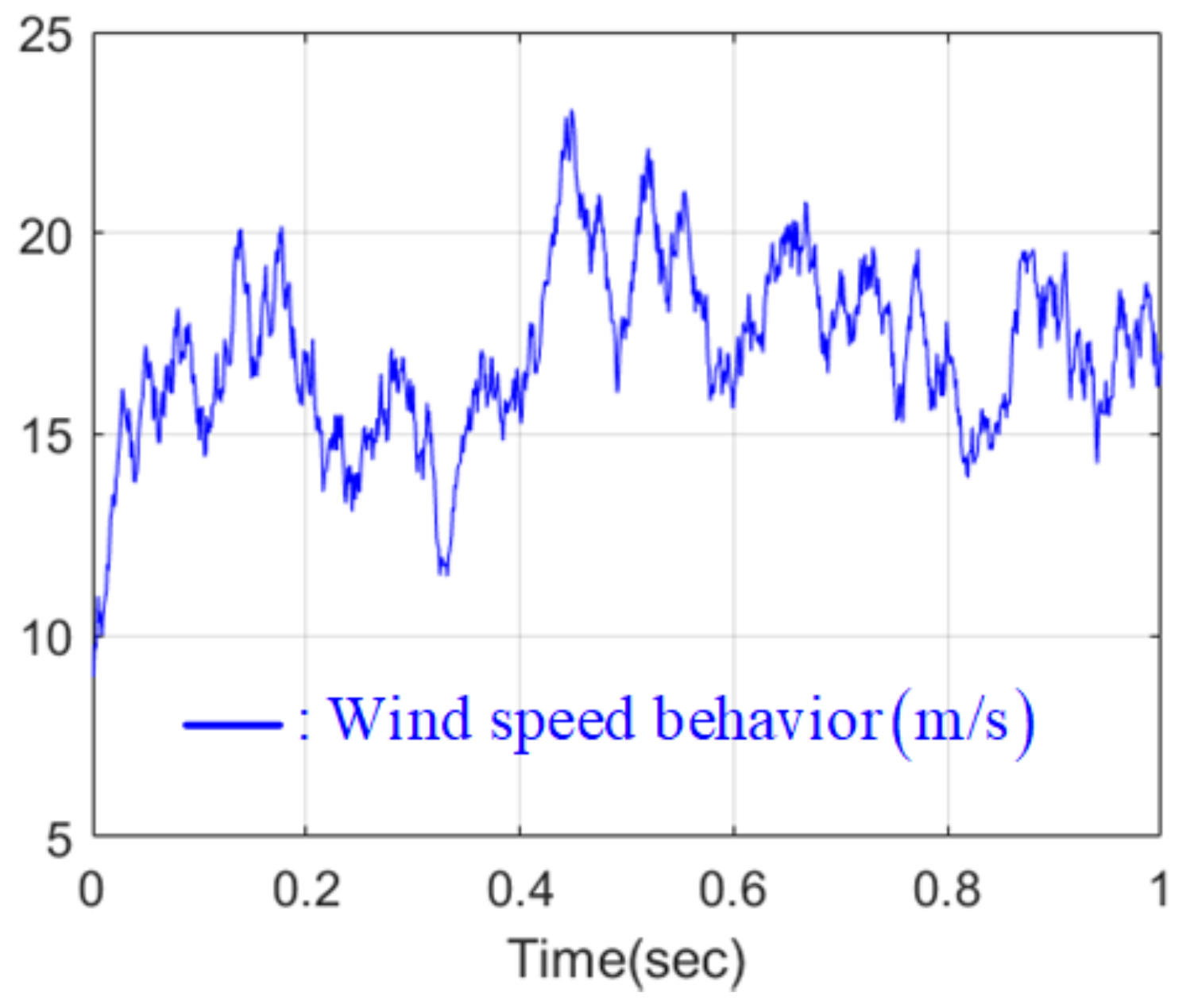
Figure 3.
Wind power generation system implementation.
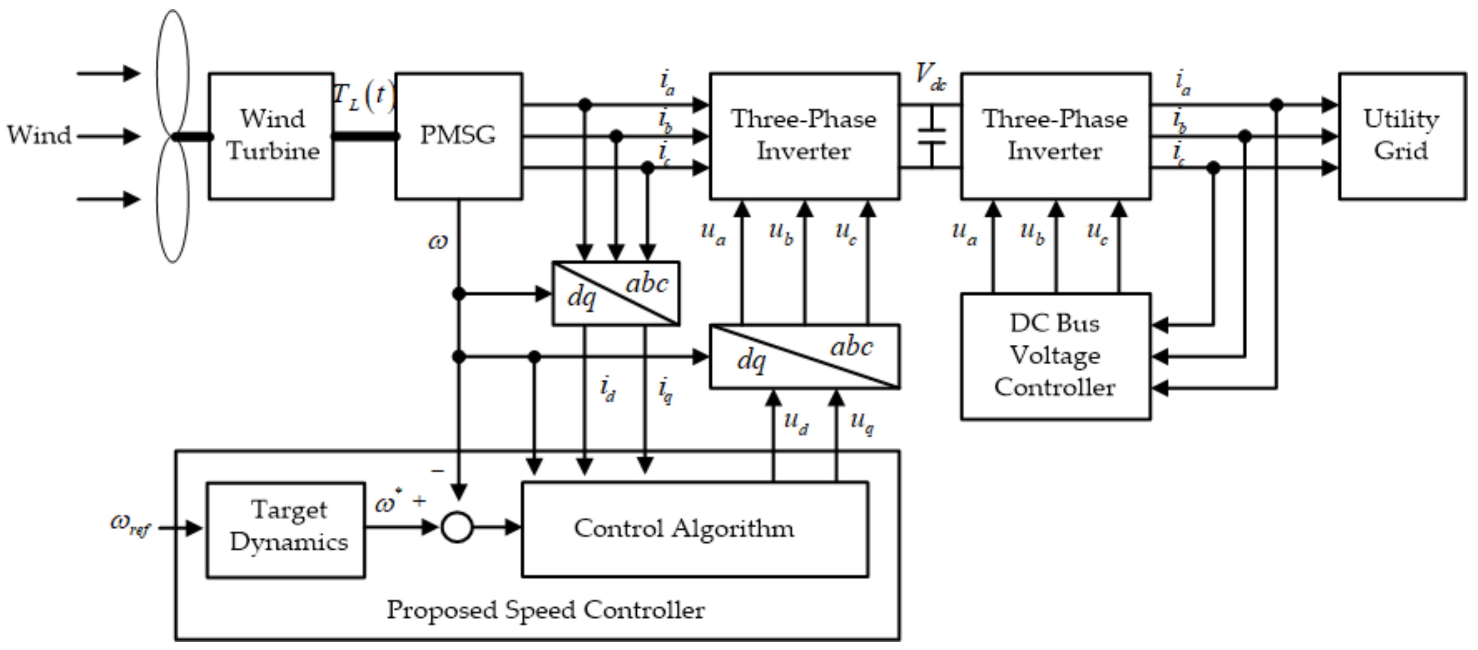
Figure 4.
Speed tracking performance comparison result with load torque behavior at cut-off frequency of Hz.
Figure 4.
Speed tracking performance comparison result with load torque behavior at cut-off frequency of Hz.

Figure 5.
d-q axis current behavior at cut-off frequency of Hz.
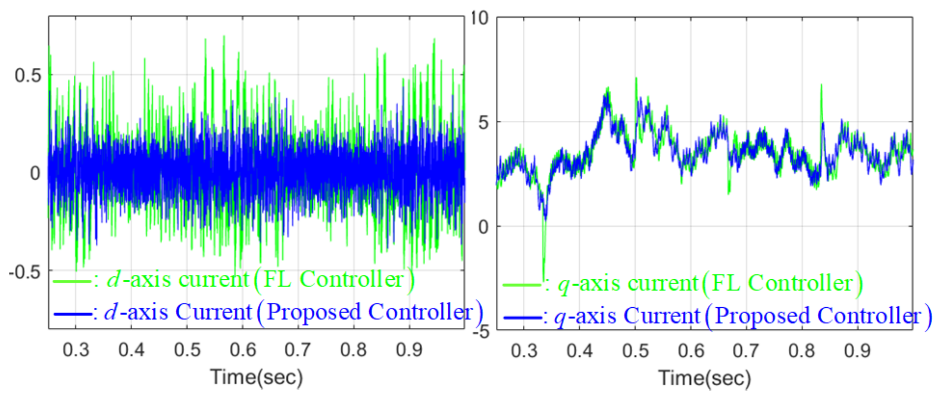
Figure 6.
Disturbance estimate behaviors.

Figure 7.
Speed tracking performance changes for various cut-off frequencies as Hz.
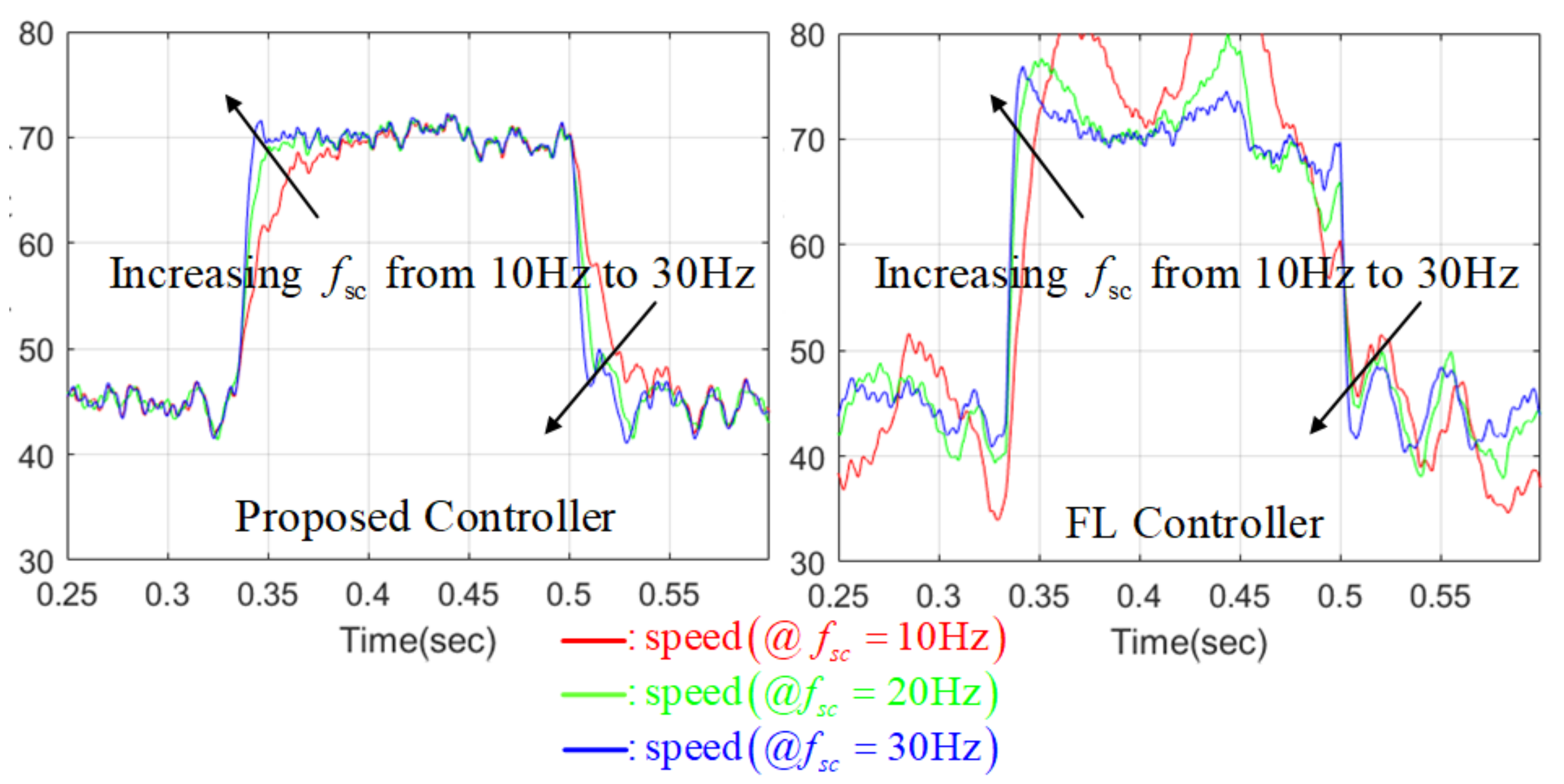
Figure 8.
Quantitative speed tracking performance comparison results.
© 2018 by the authors. Licensee MDPI, Basel, Switzerland. This article is an open access article distributed under the terms and conditions of the Creative Commons Attribution (CC BY) license (http://creativecommons.org/licenses/by/4.0/).
Share and Cite
MDPI and ACS Style
Kim, S.-K.; Lee, K.-B. Robust Offset-Free Speed Tracking Controller of Permanent Magnet Synchronous Generator for Wind Power Generation Applications. Electronics 2018, 7, 48. https://doi.org/10.3390/electronics7040048
AMA Style
Kim S-K, Lee K-B. Robust Offset-Free Speed Tracking Controller of Permanent Magnet Synchronous Generator for Wind Power Generation Applications. Electronics. 2018; 7(4):48. https://doi.org/10.3390/electronics7040048
Chicago/Turabian StyleKim, Seok-Kyoon, and Kyo-Beum Lee. 2018. "Robust Offset-Free Speed Tracking Controller of Permanent Magnet Synchronous Generator for Wind Power Generation Applications" Electronics 7, no. 4: 48. https://doi.org/10.3390/electronics7040048
Note that from the first issue of 2016, this journal uses article numbers instead of page numbers. See further details here.