Radar Waveform Recognition Based on Time-Frequency Analysis and Artificial Bee Colony-Support Vector Machine

Abstract

In this paper, a system for identifying eight kinds of radar waveforms is explored. The waveforms are the binary phase shift keying (BPSK), Costas codes, linear frequency modulation (LFM) and polyphase codes (including P1, P2, P3, P4 and Frank codes). The features of power spectral density (PSD), moments and cumulants, instantaneous properties and time-frequency analysis are extracted from the waveforms and three new features are proposed. The classifier is support vector machine (SVM), which is optimized by artificial bee colony (ABC) algorithm. The system shows well robustness, excellent computational complexity and high recognition rate under low signal-to-noise ratio (SNR) situation. The simulation results indicate that the overall recognition rate is 92% when SNR is −4 dB.

1. Introduction

Low Probability of Intercept (LPI) radar waveforms possess many characteristics. They are widely used in many fields, such as air defense radar, airborne fire control radar and beyond visual range radar and so forth. However, the detection of them is a difficult thing. Therefore, it is important to study LPI radar waveform recognition.

Many recognition methods have been put forward to recognize radar waveforms. For instance, extracting the bispectrum cascade feature to identify six kinds of waveforms (CW, LFM, NLFM, BPSK, QPSK and FSK) in [1]. Atomic Decomposition (AD) and Expectation Maximization (EM) algorithms are used to detect radar waveforms [2]. But only LFM and BPSK can be identified in this method. In [3], power spectrum accumulation and similarity theory are utilized to detect the noise frequency modulation signal. When SNR is −3 dB and the duration is 1 ms, the recognition rate is 100%. The method based on the statistics of energy for detecting noise frequency modulation signal is proposed [4]. But it has good performance only for the signals of long time. The paper [5] presents Bispestra Diagonal Slice (BDS) to distinguish four types of waveforms (including FMCW, Frank code, Costas codes and FSK/PSK). The ratio of successful recognition (RSR) is more than 93.4% when signal-to-noise ratio (SNR) ≥8 dB. In [6], random projections and sparse classification are adopted to recognize LFM, FSK and PSK. The RSR is about 90% when SNR is 0 dB. Lunden explored the system based on Choi-Williams distribution (CWD) and Wigner-Ville distribution (WVD) to distinguish eight kinds of waveforms [7]. However, the algorithm requires prior information and the RSR is 98% at SNR of 6 dB. In [8], Zhang proposes the system to recognize eight radar waveforms. The RSR is 94.7% at SNR of −2 dB and the number of features is 23. Therefore, it is a challenge for the existing methods to distinguish more radar waveforms with fewer features under high noise environment.

The system for recognizing eight LPI waveforms is proposed in this paper. The recognizable radar waveforms contain BPSK, Costas codes, LFM, P1-P4 and Frank codes. The classifier is the support vector machine (SVM) of artificial bee colony (ABC) algorithm. The features what we use are roughly divided into two types. Some features are calculated by time-domain signals and we call them time features. The other features are from time-frequency analysis and we call them time-frequency (T-F) features. Time features are extracted from the power spectral density (PSD), second order moments and cumulants and instantaneous properties. T-F features are related to WVD and CWD. Simulation results indicate that recognition rate can reach up to 92% when SNR is −4 dB.

The contributions of this paper are mainly in four aspects: (1) the recognition system is proposed and getting better results than other methods; (2) proposing three new features, that is, the ratio of peak values of WVD (${\widehat{M}}_w$), the number of extreme points (${\widehat{N}}_m$) and the oscillation amplitude of the sidelobe (${\widehat{a}}_s$); (3) the number of features of this article is less than other methods; (4) and prior information is not needed in the system.

The framework of this article is shown below. Section 2 mainly presents the structure of system. The classifier is explained in Section 3. All the features and the principle of each feature are introduced in Section 4. Section 5 conveys the simulation results and the conclusions are drawn in Section 6.

2. Recognition System Structure

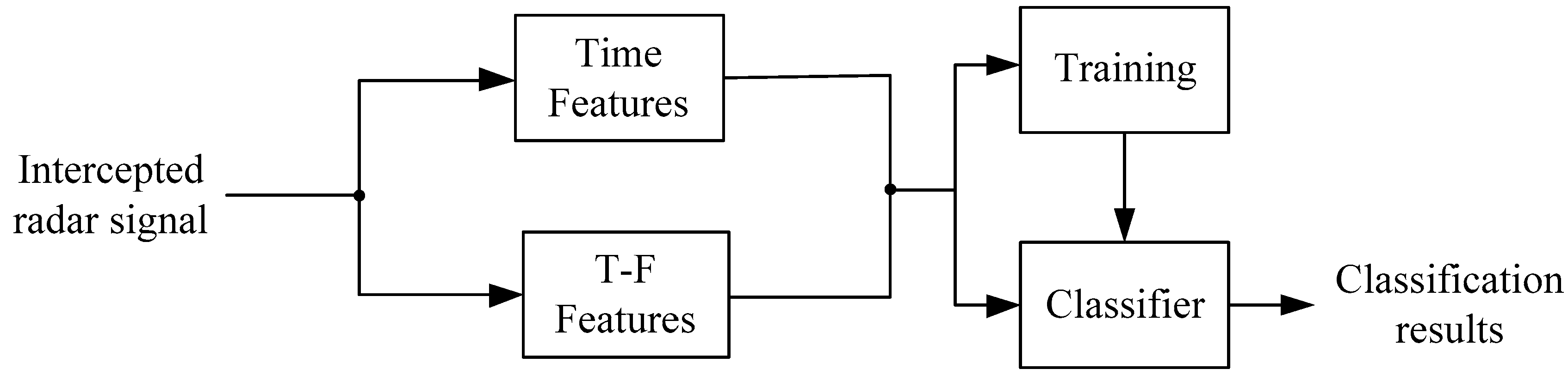
Recognition system is employed to classify the intercepted waveforms and we can obtain the category of them. Recognition System can be divided into two parts, that is, features and classifier. First of all, the features of the intercepted radar waveforms are extracted, that is, time features and T-F features. Then, to select part of the data as the training set and get the model through training. Finally, to take the rest of data as the test set and put the test set and model into the classifier to get the classified results. For more details, see Figure 1.

The intercepted signal in system can be given by

$$y\left(k\right)=x\left(k\right)+n\left(k\right)=A{e}^{j\varphi \left(k\right)}+n\left(k\right)$$

(1)

where $x\left(k\right)$ is the radar waveform. $n\left(k\right)$ is the noise and we assume it is additive white Gaussian noise (AWGN). $A$ and $\varphi \left(k\right)$ are the amplitude and phase sequence, respectively. The phase $\varphi \left(k\right)$ of BPSK, Costas, LFM and polyphase codes is listed in

Table 1. The phase of 8 radar waveforms.

Radar Waveforms	Phase $\mathit{\varphi }\left(\mathit{k}\right)$
BPSK	$\varphi \left(k\right)=2\pi f_{c}k+\theta ,\theta \in \left\{0,\pi \right\}$
Costas	$\varphi \left(k\right)=2\pi f_{s}k,f_s=\left\{f_1,f_2,\cdots ,f_{N_F}\right\}$
LFM	$\varphi \left(k\right)=2\pi \left(f_{c}k+k^2\mu /2\right)$
P1	$\varphi \left(k\right)=2\pi f_{c}k-\pi \left[\sqrt{N_c}-\left(2n-1\right)\right]\left[\left(n-1\right)\sqrt{N_c}+\left(m-1\right)\right]/\sqrt{N_c}$
P2	$\varphi \left(k\right)=2\pi f_{c}k-\pi \left[2m-1-\sqrt{N_c}\right]\left[2n-1-\sqrt{N_c}\right]/\left(2\sqrt{N_c}\right)$
P3	$\varphi \left(k\right)=2\pi f_{c}k+\pi {\left(l-1\right)}^2/N_c$
P4	$\varphi \left(k\right)=2\pi f_{c}k+\pi {\left(l-1\right)}^2/N_c-\pi \left(l-1\right)$
Frank	$\varphi \left(k\right)=2\pi f_{c}k+2\pi \left(m-1\right)\left(n-1\right)/\sqrt{N_c}$

.

In Table 1, $f_c$ is the carrier frequency. For BPSK, $\theta$ is the initial phase and its value is 0 or $\pi$. For Costas, $f_s$ is the frequency sequence and it is given by

$$f_{k+i}-f_k\ne f_{j+i}-f_j$$

where $1\le k<i<i+j\le N_F$. For LFM, $\mu$ is the slope of instantaneous frequency and it equals to the ratio of bandwidth $B$ to pulse width $\tau$. For polyphase codes, $N_c$ is the number of symbols, $m=1,2,3,\cdots ,\sqrt{N_c}$, $n=1,2,3,\cdots ,\sqrt{N_c}$ and $l=1,2,3,\cdots ,N_c$. In addition, $\sqrt{N_c}$ must be the even for P2 codes.

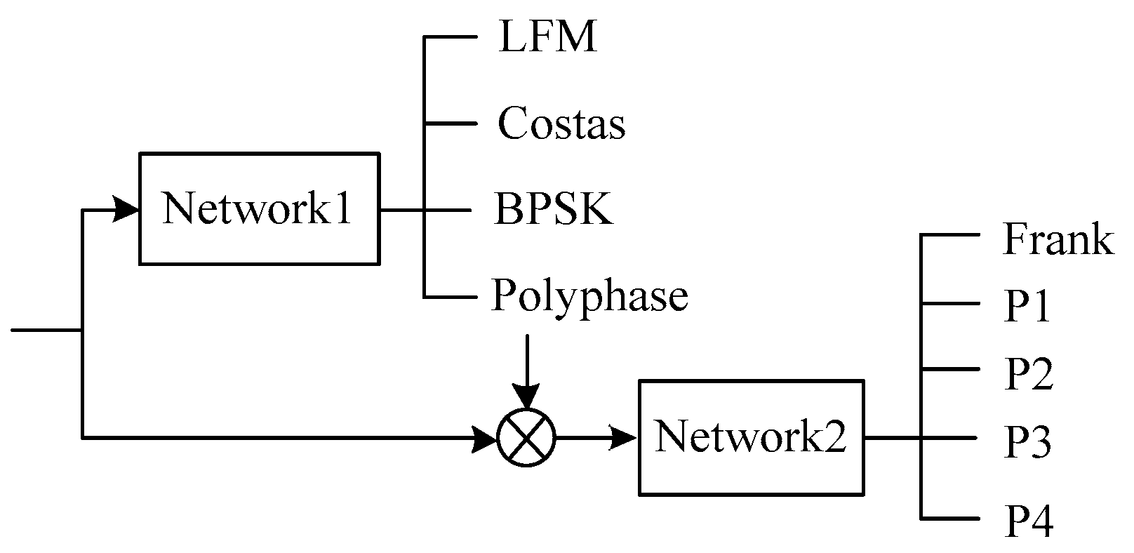
The classifier in the system is composed of network1 and network2. It can classify eight waveforms. BPSK, Costas and LFM can be directly classified by network1 and network2 does not work at this time. When the signal is deemed to be polyphase codes (P1-P4 and Frank codes) by network1, then network2 is used to classify polyphase codes in detail. The purpose of adopting two classification networks is to reduce input features and improve the classification accuracy. For more details, see Figure 2.

3. Classifier

The classifier of the system is ABC-SVM and it is applied in two networks. In SVM, parameter selection has a significant impact on the classification accuracy of model. Therefore, ABC algorithm is adopted to find the optimal parameters of SVM.

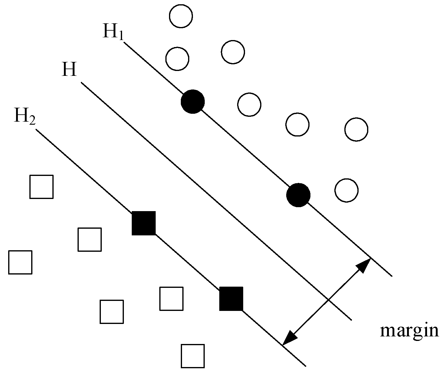
In SVM [9], the hyperplane is used to separate different types of data because the symbols on both sides of the hyperplane are different. When the interval between hyplane and data is greater, the confidence of classification is greater. Therefore, the key question for SVM is to find the hyperplane that can separate the training data without mistakes and make the geometric interval (margin) is the largest, that is optimal separating hyperplane. The SVM about two classes and linear separable problems is shown in Figure 3. We assume that the number of samples is $l$, the training vectors ${\mathbf{x}}_i\in R^n$, $i=1,\dots ,l$, an indicator vector $\mathbf{y}\in R^l$ and $y_i\in \left\{1,-1\right\}$. The hyperplane is $\left(\mathsf{\omega }•\mathbf{x}\right)+b=0$. Therefore, the problem of solving the optimal hyperplane is turned into an optimization problem [10]:

$$\begin{array}{ll}\hfill \underset{\mathsf{\omega },b,\xi }{\min }& \frac{1}{2}{\mathsf{\omega }}^T\mathsf{\omega }+C{\displaystyle \sum _{i=1}^l{\xi }_i}\hfill \\ \hfill \mathrm{subject}\mathrm{to}& y_i\left({\mathsf{\omega }}^T\varphi \left({\mathbf{x}}_i\right)+b\right)\ge 1-{\xi }_i,\hfill \\ & {\xi }_i\ge 0,i=1,\dots ,l,\hfill \end{array}$$

(2)

where $\omega$ is the normal vector of hyperplane, $\xi$ and $b$ mean the slack variable and threshold, respectively. $C$ is the error penalty factor and it need to be designed. $\varphi \left(x_i\right)$ is the result of non-linear transformation of $x_i$ in the new space. Then the optimization problem is converted to its dual problem by the method of Lagrange [10]:

$$\begin{array}{cc}\hfill \underset{\alpha }{\min }& \frac{1}{2}{\mathsf{\alpha }}^T\mathbf{Q}\mathsf{\alpha }-{\mathbf{e}}^T\mathsf{\alpha }\hfill \\ \hfill \mathrm{subject}\mathrm{to}& {\mathbf{y}}^T\mathsf{\alpha }=0,\hfill \\ & 0\le {\alpha }_i\le C,i=1,\dots ,l,\hfill \end{array},$$

(3)

where $\alpha$ is the Lagrange multiplier, $\mathbf{e}$ is a vector of all ones and $\mathbf{Q}$ is an positive semidefinite matrix, that is, $Q_{ij}=y_i{y}_{j}K\left({\mathbf{x}}_i,{\mathbf{x}}_j\right)$. $K\left({\mathbf{x}}_i,{\mathbf{x}}_j\right)$ is the kernel function and it is influenced by the kernel function parameter $\sigma$. It can be given by

$$K\left({\mathbf{x}}_i,{\mathbf{x}}_j\right)=\varphi {\left({\mathbf{x}}_i\right)}^T\varphi \left({\mathbf{x}}_j\right).$$

(4)

When the Formula (3) is calculated, the solution ${\alpha }^{\ast }$ can be obtained and the vector $\mathsf{\omega }$ is also be confirmed, that is,

$${\mathsf{\omega }}^{\ast }={\displaystyle \sum _{i=1}^l{\alpha }_i^{\ast }{y}_i\varphi \left({\mathbf{x}}_i\right)},$$

(5)

$b$ is estimated by

$$y_i\left({\displaystyle \sum _{i=1}^l{\alpha }_i^{\ast }K\left({\mathbf{x}}_i,{\mathbf{x}}_j\right)+b^{\ast }}\right)-1=0$$

(6)

and the classified decision function is [10]

$$f\left(\mathbf{x}\right)=\mathrm{sgn}\left({\mathsf{\omega }}^{\ast }\varphi \left(\mathbf{x}\right)+b^{\ast }\right)=\mathrm{sgn}\left({\displaystyle \sum _{i=1}^l{\alpha }_i^{\ast }{y}_{i}K\left({\mathbf{x}}_i,\mathbf{x}\right)}+b^{\ast }\right).$$

(7)

Thus, the choice of $C$ and $\sigma$ has an important impact on the classification results of SVM [11,12].

ABC algorithm proposed by Karaboga [13] is utilized to evaluate the parameters of SVM in this paper. ABC is a global optimization algorithm and its purpose is to search the optimum solution of problems by imitating the behavior of honey bee swarm in nature. ABC algorithm is composed of scouts, onlookers and employed bees. The quantity of employed bees is one half of the populations and the amount of food sources (solutions) is equal to the employed bees. The specific process is described as below [14]: the first step is to initialize the food sources. Then, employed bees search around the food sources in some way to find new sources and choose the better ones according to the nectar amount (fitness). Next, onlookers pick good food sources further on the basis of the message of employed bees and confirm the quantity. If nectar amount of that food source is not improved within given steps, the employed bee will turn into the scouts. The task of scouts is to find new food sources. When the cycle reaches the terminating condition, the optimal food source will be received. For more details, see

Table 2. The main steps of artificial bee colony (ABC) algorithm.

Steps	Features
1	Initialize Stage
2	repeat
3	Employed Bees Stage
4	Onlooker Bees Stage
5	Scout Bees Stage
6	Memorize the best food source
7	until cycle = Maximum Cycle Number (MCN)

.

In initialize stage, we assume the number of solutions is $SN$ and the solutions are randomly generated. The quantity of employed bees is $SN$, as well. Initial solutions are given by

$$x_{ij}=x_{\min ,j}+rand\left(0,1\right)\left(x_{\max ,j}-x_{\min ,j}\right),$$

(8)

where $x_i\left(i=1,2,\dots ,SN\right)$ is a D-dimensional vector, $D$ represents the amount of optimized parameters and $j\in \left\{1,2,\dots ,D\right\}$. $x_{ij}$ is the $j$th parameter of $x_i$.

In employed bees stage, employed bees calculate the fitness and search around the initial values to find new solutions. If new fitness is more than the original, employed bees will remember the new solutions and forget the original ones. When employed bees finish seeking and return to the beehives, they share information with onlookers. The formula of searching new solutions is given by

$$v_{ij}=x_{ij}+{\phi }_{ij}\left(x_{ij}-x_{kj}\right),$$

(9)

where $j\in \left\{1,2,\dots ,D\right\}$, $k\in \left\{1,2,\dots ,SN\right\}$ and $k\ne i$. ${\phi }_{ij}$ is a random number of $[-1,1]$.

In the onlooker bees stage, onlookers select solutions according to the received message with a certain probability. Then, onlookers search the solutions in the same way of employed bees to produce new solutions. If new fitness is better, we will replace the previous. The probability of onlookers to choose the solutions is given by

$$P_i=\frac{fit\left(x_i\right)}{{\displaystyle \sum _{n=1}^{SN}fit\left(x_n\right)}},$$

(10)

where $fit\left(x_i\right)$ is the fitness of the $i$th solution.

In the scout bees stage, if the solution $x_i$ is not improved within $limit$, it will be abandoned. The employed bees of that position will turn into the scouts and a new solution is produced by Formula (8). When the number of cycles reaches the maximum cycle number (MCN), the best solution will be obtained.

4. Features Extraction

Feature extraction is an important step in the recognition system and it is closely related to the classification results. These features are divided into time features and T-F features. Time features means these features are based on the power spectral density (PSD), second order statistics and instantaneous characteristics. T-F features are bound up with WVD and CWD. The process of extracting T-F features need to be explained. The whole features of two networks are illustrated in

Table 3. Features of network1 and network2.

Numbers	Features	Network1	Network2
1	${\widehat{M}}_{10}$	$\surd$
2	${\widehat{M}}_{20}$	$\surd$
3	${\widehat{C}}_{20}$	$\surd$
4	${\gamma }_1$	$\surd$
5	${\gamma }_2$	$\surd$
6	${\widehat{\sigma }}_{\varphi }$	$\surd$
7	${\widehat{\sigma }}_f$	$\surd$
8	${\widehat{M}}_w$	$\surd$
9	$N_{obj}$	$\surd$
10	$t_{\max }$	$\surd$	$\surd$
11	${\widehat{\sigma }}_{obj}$	$\surd$	$\surd$
12	${\widehat{\theta }}_{\max }$		$\surd$
13	${\widehat{a}}_s$		$\surd$
14	${\widehat{N}}_m$		$\surd$

.

4.1. Time Features

4.1.1. Features Related to Moments and Cumulants

Second order moments and cumulants are suitable for discriminating BPSK from others. Therefore, two features about Moments and Cumulants are proposed.

The nth moment of the signal $y\left(k\right)$ is given by

$${\widehat{M}}_{nm}=\left|\frac{1}{N}{\displaystyle \sum _{k=0}^{N-1}{y}^{n-m}\left(k\right){\left(y^{*}\left(k\right)\right)}^m}\right|,$$

(11)

where $N$ is the size of signals. $m$ is the amount of conjugated sections. ${\widehat{M}}_{10}$ and ${\widehat{M}}_{20}$ are obtained by this formula.

The nth order cumulant can be computed through [15,16]

$${\widehat{C}}_{nm}=\left|\frac{1}{N}{\displaystyle \sum _{k=0}^{N-1}{\left(y\left(k\right)-{\widehat{M}}_{10}\right)}^{n-m}{\left(y^{*}\left(k\right)-{\widehat{M}}_{10}\right)}^m}\right|$$

(12)

where ${\widehat{M}}_{10}$ is calculated by Formula (11). ${\widehat{C}}_{20}$ can be received by Formula (12).

4.1.2. Features Related to Power Spectral Density (PSD)

PSD expresses the frequency domain distribution of signal energy. Hence the PSD features can be estimated as [6]

$${\gamma }_m=\frac{1}{N}\underset{n}{\max }\left\{\frac{1}{N}{\left|{\displaystyle \sum _{k=0}^{N-1}{\tilde{y}}^m\left(k\right)e^{-j2\pi nk/N}}\right|}^2\right\},$$

(13)

where $\tilde{y}\left(k\right)$ is given by

$$\tilde{y}\left(k\right)=\frac{y\left(k\right)}{\sqrt{{\widehat{M}}_{21}-{\sigma }_{\epsilon }^2}},$$

(14)

where ${\sigma }_{\epsilon }^2$ is the variance of noise. ${\widehat{M}}_{21}$ is the third moment and can be received by Formula (11).

${\gamma }_1$ and ${\gamma }_2$ can be explored by Formula (13). ${\gamma }_1$ applies to distinguish BPSK from Costas codes. The squared complex envelope is constant for BPSK, therefore, ${\gamma }_2$ is beneficial to differentiate between BPSK and other waveforms.

4.1.3. Features Related to Instantaneous Properties

It has good effect to discriminate the frequency modulation signals from the phase modulation signals by the instantaneous properties of radar waveforms. Therefore, two features based on the instantaneous frequency and instantaneous phase are presented.

${\widehat{\sigma }}_{\varphi }$ means the standard deviation of the absolute of instantaneous phase and it can be given by [17]

$${\widehat{\sigma }}_{\varphi }=\sqrt{\frac{1}{N}\left({\displaystyle \sum _{k=0}^{N-1}{\varphi }^2\left(k\right)}\right)-{\left(\frac{1}{N}{\displaystyle \sum _{k=0}^{N-1}\left|\varphi \left(k\right)\right|}\right)}^2},$$

(15)

where $\varphi \left(k\right)$ indicates the instantaneous phase of radar waveforms and $\mathrm{N}$ still implies the amount of samples. The range of $\varphi \left(k\right)$ is between $-\pi$ and $\pi$.

${\widehat{\sigma }}_f$ means the standard deviation of the absolute of normalized centered instantaneous frequency and it can be estimated as

$${\widehat{\sigma }}_f=\sqrt{\frac{1}{N_f}{\displaystyle \sum _{k=0}^{N-1}{\tilde{f}}^2\left(k\right)}-{\left(\frac{1}{N_f}{\displaystyle \sum _{k=0}^{N-1}\left|\tilde{f}\left(k\right)\right|}\right)}^2},$$

(16)

where $\tilde{f}\left(k\right)$ indicates the normalized centered instantaneous frequency and the size of $\tilde{f}\left(k\right)$ is $N_f$. It can be obtained through the following process:

• to compute the instantaneous phase, that is, $\varphi \left(k\right)$;
• to acquire the unwrapped instantaneous phase ${\varphi }_u\left(k\right)$ by $\varphi \left(k\right)$;
• to calculate the instantaneous frequency $f\left(k\right)$, that is, $f\left(k\right)={\varphi }_u\left(k\right)-{\varphi }_u\left(k-1\right)$;
• to calculate the mean of $f\left(k\right)$, that is, ${\mu }_f$;
• to get $\tilde{f}\left(k\right)$ by $\tilde{f}\left(k\right)=\left(f\left(k\right)-{\mu }_f\right)/\left(\max \left|f\left(k\right)-{\mu }_f\right|\right)$.

4.2. T-F Features

4.2.1. Feature Related to Wigner-Ville Distribution (WVD)

WVD [18] was proposed by Wigner. It is used to describe the signal distribution in time and frequency domain. Hence the WVD of $x\left(t\right)$ is given by [19]

$$W_x\left(t,\omega \right)=\frac{1}{2\pi }{\displaystyle {\int }_{-\infty }^{\infty }x\left(t+\frac{1}{2}\tau \right)x^{*}\left(t-\frac{1}{2}\tau \right)e^{-j\omega \tau }d\tau },$$

(17)

where $t$ is time variable and $\mathsf{\omega }$ is frequency variable.

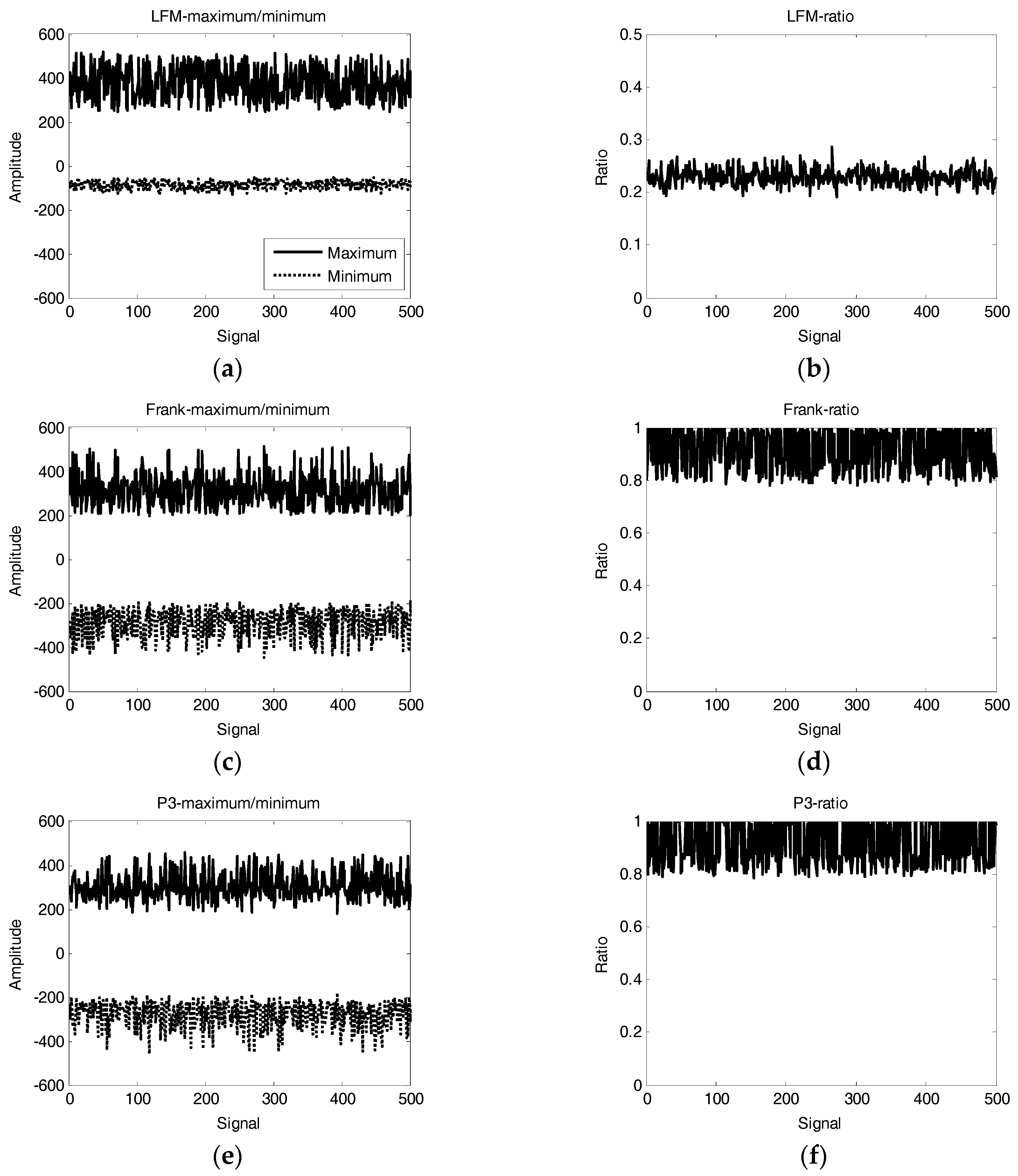
The feature based on the cross terms of WVD is proposed. It is utilized to discriminate LFM from Frank code and P3 code. For a single-component LFM of finite length, there are no cross terms and the amplitude of the WVD is related to the sampling signal [20]. Therefore, the absolute of the ratio of the minimum value to the maximum value is about 0.25. For Frank code and P3 code, the amplitude of the cross terms is about two times the signal terms in WVD [21]. That means the maximum and minimum value are both related to the cross terms. The amplitude of cross terms contains cosine function [22]. Therefore, the absolute of the ratio of the minimum to the maximum is about 1. For LFM, Frank and P3, the maximum, minimum and the ratio of 500 signals at SNR = 6 dB are displayed in Figure 4.

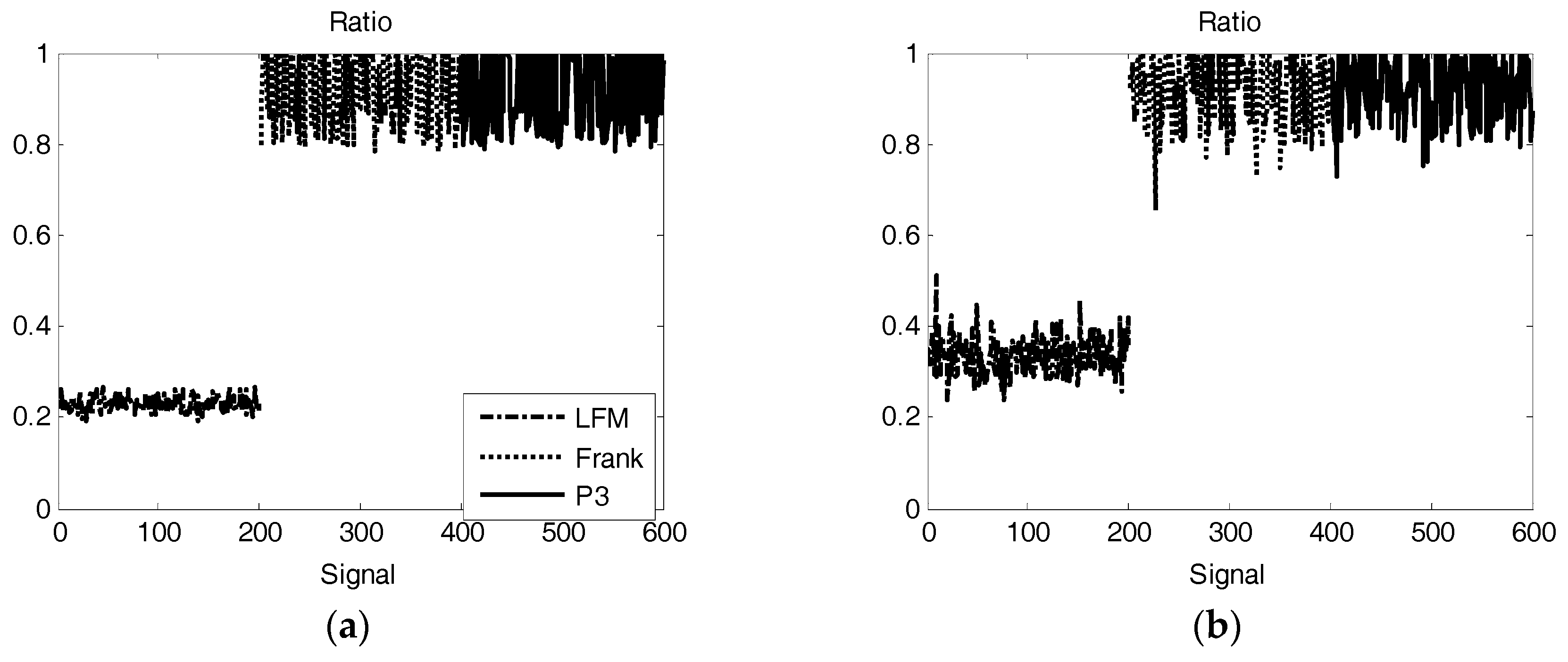
The ratio of LFM, Frank and P3 at diverse SNR is displayed in Figure 5. When SNR is 6 dB, the ratio of LFM is about 0.24 and it is very close to 0.25. The ratio of Frank and P3 is about 0.9 and it is very close to 1. When SNR is −4 dB, the ratio of LFM is about 0.3. It is also close to 0.25. The ratio of Frank and P3 is about 0.9. It is also close to 1. That indicates the differences between LFM and the other waveforms (Frank and P3). The feature related to this ratio is proposed, that is, ${\widehat{M}}_w$.

${\widehat{M}}_w$ is given by:

$${\widehat{M}}_w=\frac{abs\left(W_{\min }\right)}{W_{\max }},$$

(18)

where $W_{\min }$ and $W_{\max }$ are the minimum and maximum amplitudes in $W_x\left(t,\omega \right)$, respectively. $W_x\left(t,\omega \right)$ can be calculated by Formula (17).

4.2.2. Choi-Williams Distribution (CWD)

CWD belongs to the Cohen time-frequency distribution [23]. It is given by:

$$C_f\left(t,\omega ,\varphi \right)=\frac{1}{2\pi }{\displaystyle \iiint e^{j\left(\xi \mu -\tau \omega -\xi t,\tau \right)}\varphi \left(\xi ,\tau \right)x\left(\mu +\tau /2\right)x^{*}\left(\mu -\tau /2\right)d\mu d\tau d\xi },$$

(19)

where $t$ indicates the time variable and $\omega$ indicates the frequency variable. $\varphi \left(\xi ,\tau \right)$ means the kernel function and it can reduce the cross terms. $\varphi \left(\xi ,\tau \right)$ is given by [24]

$$\varphi \left(\xi ,\tau \right)=e^{-{\xi }^2{\tau }^2/\sigma },$$

(20)

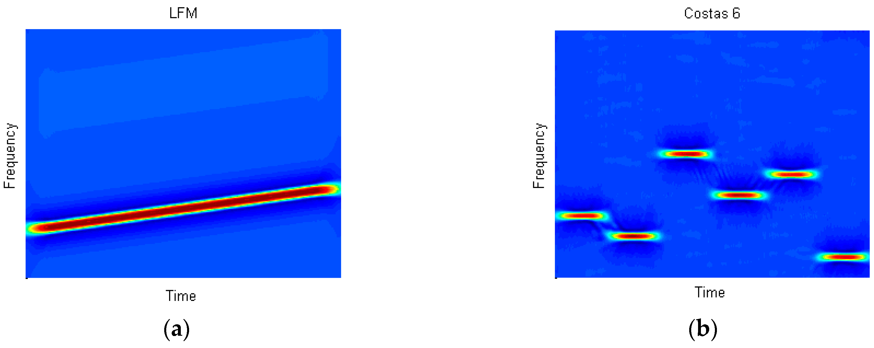
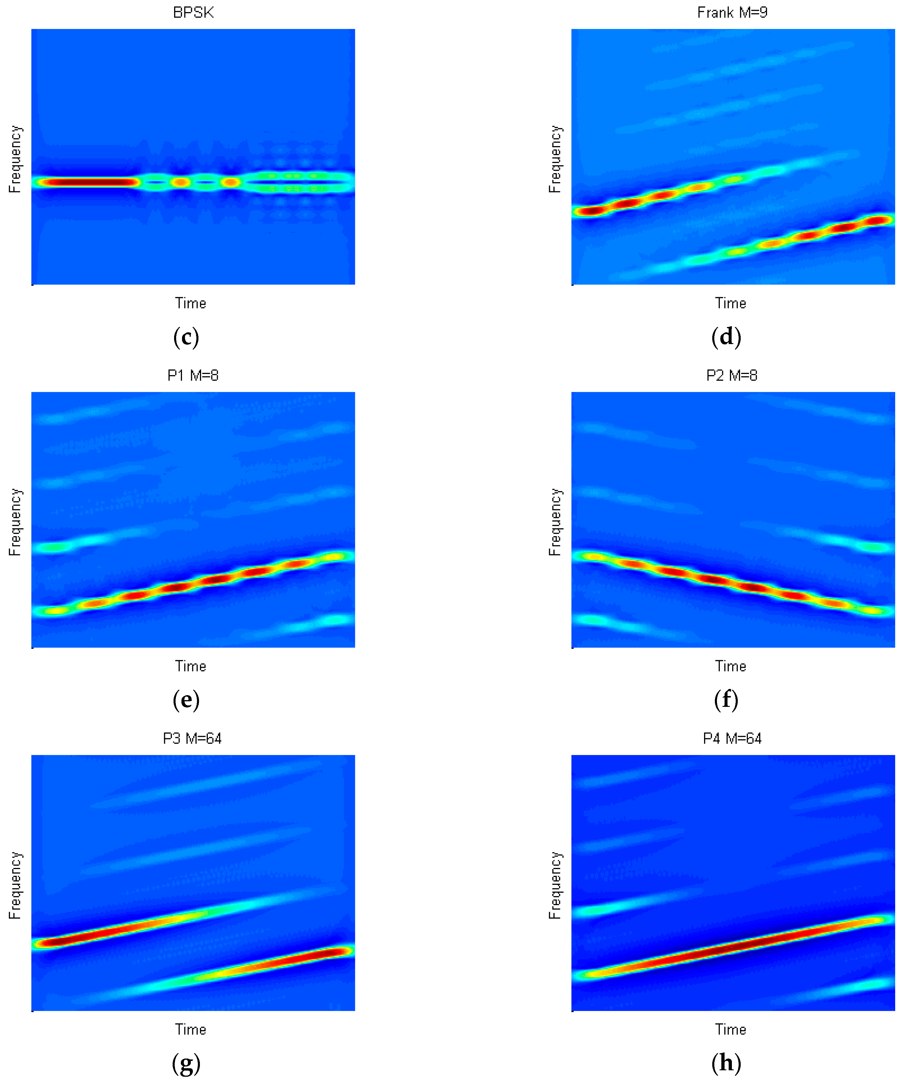
where $\sigma \left(\sigma >0\right)$ is the scaling factor and its value is set to 1 in this paper. The two-dimensional results of CWD of eight radar waveforms are displayed in Figure 6.

4.2.3. Preprocessing of the CWD Image

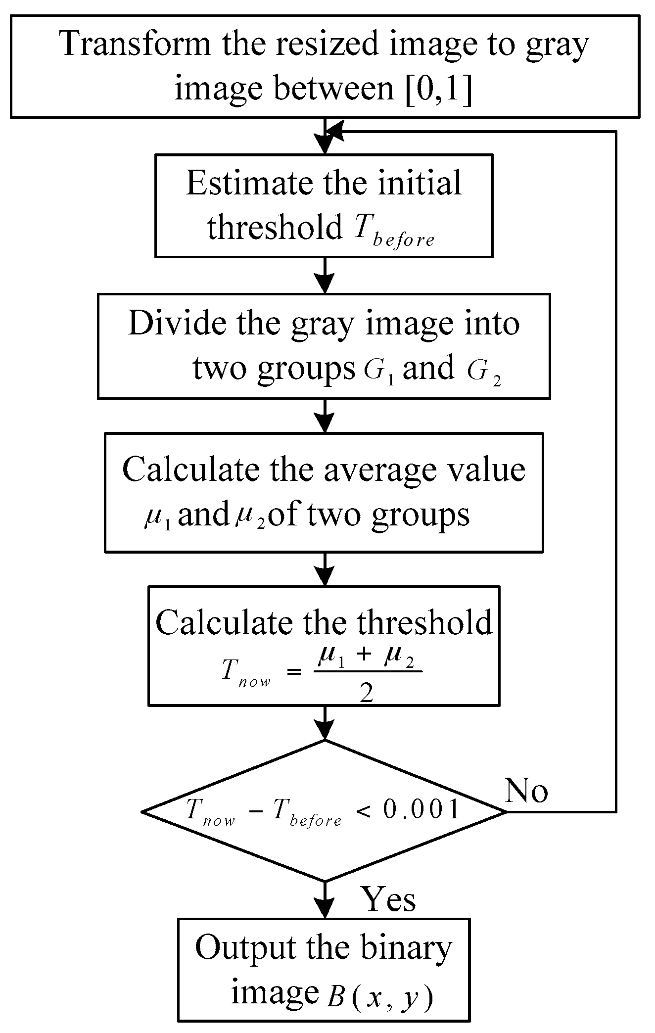
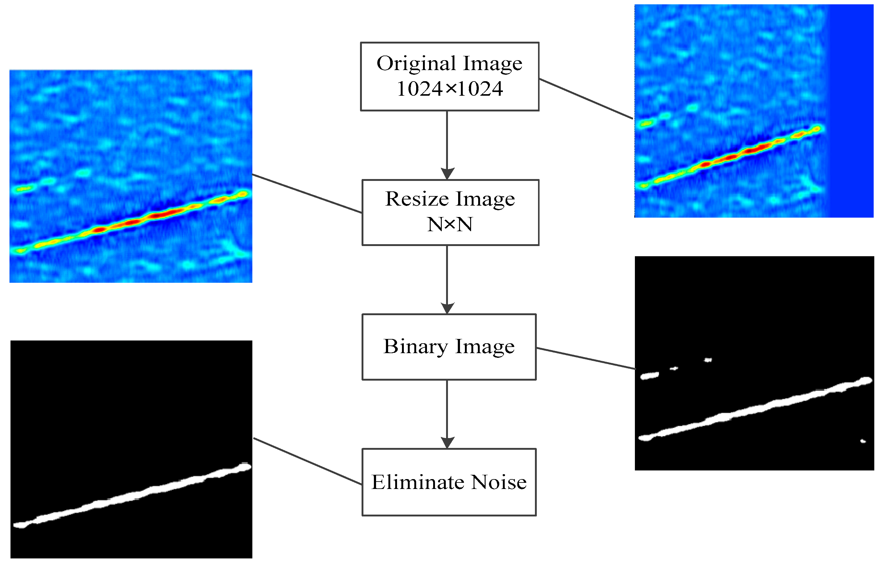
The next step is to calculate the features of the CWD image. Before doing that, the results of CWD need to be processed. The specific operations are as follows [8]:

• make the CWD transformation of 1024 points for the signals whose sampling numbers are less than 1024 and zero padding is used to deal with waveforms;
• resize the size of the CWD image to $N\times N$ to reduce the computation cost;
• the global threshold algorithm [25] is used to transform the resized CWD image into binary image and the procedure is illustrated in Figure 7;
• remove part of the binary image that is less than 10% of the size of the largest part to eliminate noise and then get the processed image.

For P4 code, the processing procedure of the CWD image at SNR = −6 dB is displayed in Figure 8.

4.2.4. CWD Features

The region consisting of pixels with the same pixel value and adjacent positions is called connected domain. For the CWD image of each waveform, P3 and Frank possess two connected domains, P1, P4 and LFM possess one domain and Costas has different results. Therefore, the amount of connected domains in binary image is a very helpful feature. In this article, that feature is $N_{obj}$. It means the amount of domains that greater than 20% of maximum component.

Next feature indicates the position of the maximum energy in the time domain of image, that is,

$$t_{\max }=\frac{1}{N-1}\arg \underset{t}{\max }\left\{C_{N\times N}\left(t,\omega \right)\right\},$$

(21)

where $C_{N\times N}\left(t,\omega \right)$ is the resized CWD image.

${\widehat{\sigma }}_{obj}$ and ${\widehat{\theta }}_{\max }$ represent the standard deviation of the length of domains and the rotate angle of the greatest domain, respectively. ${\widehat{\sigma }}_{obj}$ has a good effect on separating “stepped waveform” (Frank and P1 codes) from “linear waveform” (P3, P4 and LFM). ${\widehat{\theta }}_{\max }$ can select P2 code from others because only the slope of P2 is negative. The calculation process can be illustrated as below [8]:

• for every domain, $k=1,2,\dots ,N_{obj}$;
  • extract the domain of $\mathrm{k}$ in binary image;
  • rotate the domain of $\mathrm{k}$ through the nearest neighbor interpolation until it is vertical to the lateral axis and denoted by $B_r\left(x,y\right)$;
  • compute the row sum $\mathrm{r}\left(\mathrm{x}\right)$, that is,

    $$r\left(x\right)={\displaystyle {\sum }_{y=0}^{N-1}{B}_r\left(x,y\right)},x=0,1,2,\dots ,N-1$$
  • normalize $r\left(x\right)$, that is, $\widehat{r}\left(x\right)=r\left(x\right)/\max \left\{r\left(x\right)\right\}$;
  • compute standard deviation of $\widehat{r}\left(x\right)$, that is,

    $${\widehat{\sigma }}_{k,obj1}=\sqrt{1/N{\displaystyle {\sum }_x{\widehat{r}}^2\left(x\right)}-{\left(\left(1/N\right){\displaystyle {\sum }_x\widehat{r}\left(x\right)}\right)}^2}$$
• calculate and output the angle of rotation of the largest object ${\widehat{\theta }}_{\max }$;
• calculate and output the mean ${\widehat{\sigma }}_{obj}$ of ${\widehat{\sigma }}_{k,obj1}$, that is,

  $${\widehat{\sigma }}_{obj}=\left({\displaystyle {\sum }_{k=1}^{N_{obj1}}{\widehat{\sigma }}_{k,obj1}}\right)/N_{obj1}$$

Next step is to extract the framework of maximum domain in binary image and estimate its linear tendency by the minimal square error method. The vector $f_n$ can be obtained by removing its linear tendency in framework. Then to compute the autocorrelation function of $f_n$, that is,

$$c\left(m\right)={\displaystyle {\sum }_k{f}_n\left(k\right)f_n\left(k-m\right)},m=0,1,\dots ,M-1,$$

(22)

where $c\left(m\right)$ is the autocorrelation function of $f_n$ and $M$ is the length of $f_n$.

Some characteristics of $c\left(m\right)$ can be utilized to distinguish P1 code from P4 code. The framework of the maximum domain, the linear tendency of framework, $f_n$ and $c\left(m\right)$ of P4 and P1 at SNR = 6 dB are displayed in Figure 9.

We present two new features which are bound up $\mathrm{c}\left(\mathrm{m}\right)$, that is, ${\widehat{a}}_s$ and ${\widehat{N}}_m$. They are used to distinguish P1 from P4.

${\widehat{a}}_s$ is the oscillation amplitude of the sidelobe in $c\left(m\right)$, that is,

$${\widehat{a}}_s=abs\left(s_{\max }\right)+abs\left(s_{\min }\right),$$

(23)

where $s_{\max }$ and $s_{\min }$ are the maximum and minimum of sidelobe in $c\left(m\right)$,respectively.

${\widehat{N}}_m$ is the number of extreme points in, that is,

$${\widehat{N}}_m=\min \left(N_{\max },N_{\min }\right),$$

(24)

where $N_{\max }$ means the amount of maxima in $c\left(m\right)$ and $N_{\min }$ is the number of minima in $c\left(m\right)$.

5. Simulation Results and Discussion

5.1. Create Signals

The simulation conditions of eight radar waveforms are introduced in this section. Before creating the waveforms, we suppose the noise is additive white Gaussian noise (AWGN). The definition of SNR is $SNR=10{\log }_{10}\left(P_s/P_n\right)$, where $P_s$ indicates the signal power and $P_n$ indicates the noise power. $\mathrm{U}(\cdot )$ means the ratio of frequency. For example, the initial frequency $f_0$ is 1500 and the sampling frequency $f_s$ is 12000. So, the ratio of frequency is $\mathrm{U}(f_0/f_s)=\mathrm{U}(1/8)$. For BPSK, the range of carrier frequency $f_c$ is from $\mathrm{U}(1/8)$ to $\mathrm{U}(1/4)$ and the barker codes is 7, 11 or 13; for Costas codes, the amount of frequency $N_s$ changes from 3 to 6, the basic frequency $f_{\min }$ is $\mathrm{U}(1/24)$ and the number of samples $N$ is from 512 to 1024; for LFM, the initial frequency $f_0$ is $\mathrm{U}(1/16,1/8)$, the range of bandwidth $\mathsf{\Delta }f$ is the same as $f_0$ and the number of samples $N$ is as large as Costas codes; For polyphase codes, the carrier frequency $f_c$ is also $\mathrm{U}(1/8,1/4)$, $\mathrm{M}$ indicates the step frequency and $N_c$ indicates the coding length of signals. More details are illustrated in

Table 4. Parameters of each waveform.

Radar Waveforms	Parameter	Parameter Values
	$f_s$	1
BPSK	$f_c$	$\mathrm{U}(1/8,1/4)$
	$N_c$	7, 11, 13
Costas codes	$N_s$	[3, 6]
	$f_{\min }$	$\mathrm{U}(1/24)$
	$N$	[512, 1024]
LFM	$f_0$	$\mathrm{U}(1/16,1/8)$
	$\mathsf{\Delta }f$	$\mathrm{U}(1/16,1/8)$
	$N$	[512, 1024]
P1 and Frank codes	$f_c$	$\mathrm{U}(1/8,1/4)$
	$M$	[6, 12]
P2 code	$f_c$	$\mathrm{U}(1/8,1/4)$
	$M$	2 $\times$ [3, 6]
P3 and P4 codes	$f_c$	$\mathrm{U}(1/8,1/4)$
	$N_c$	2 $\times$ [20, 65]

.

5.2. Experiment Results with SNR

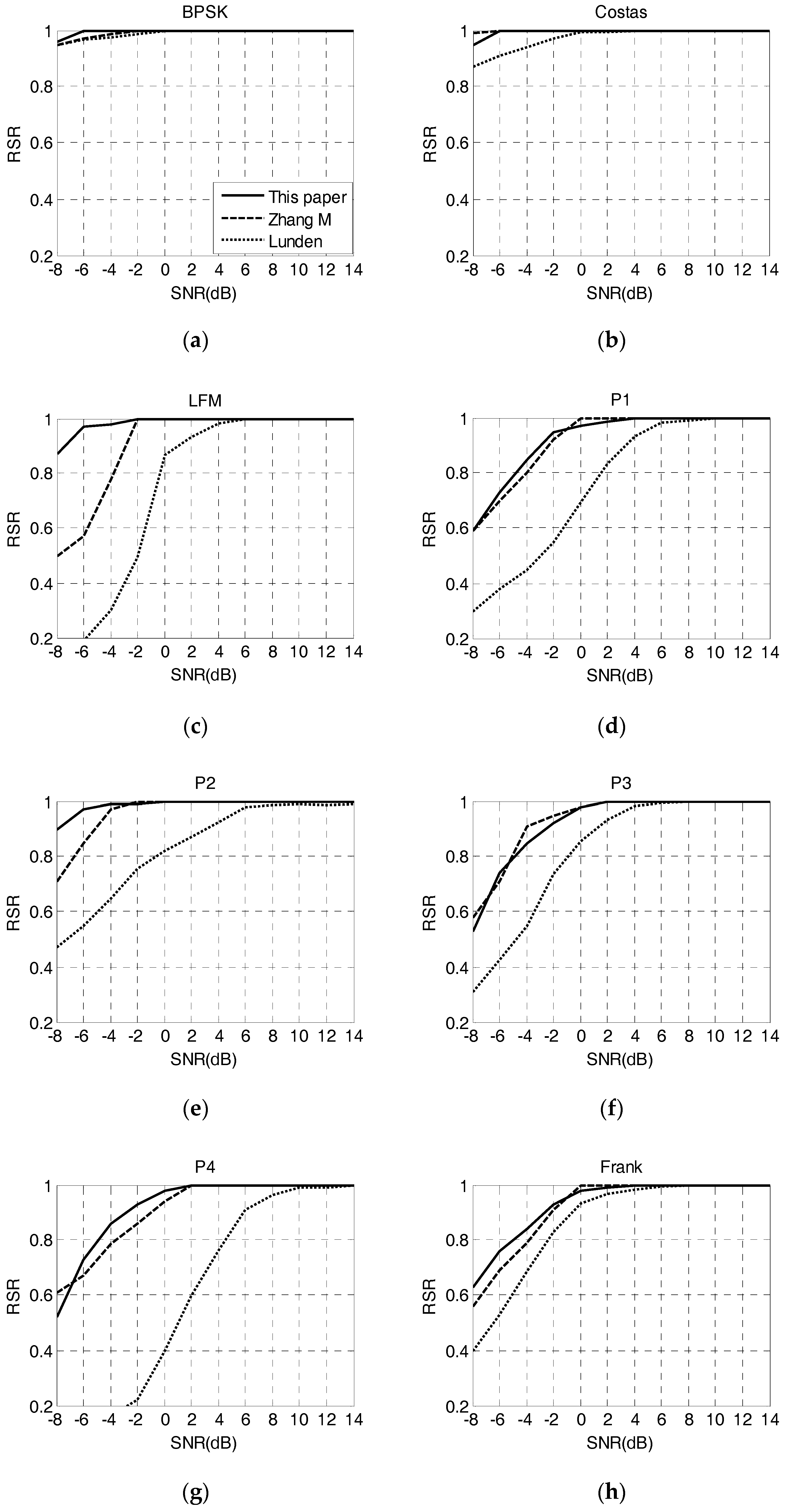
In order to make experiments on the classification of eight kinds of radar waveforms, 1000 sets of each waveform are obtained. 90% of them are employed to practice and the remaining is regarded as the test set. The range of SNR is from −8 dB to 14 dB. The RSR in this article is compared with Zhang [8] and Lunden [7] system.

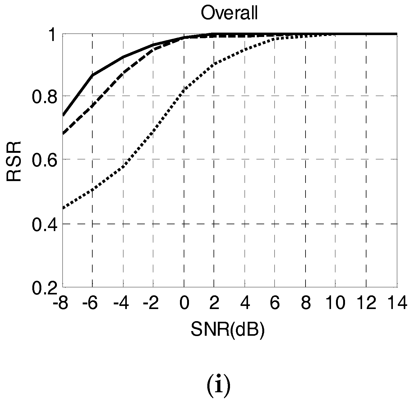
Figure 10 shows the recognition accuracy at different SNR from this paper and from Zhang’s and Lunden’s studies. For BPSK, LFM and P2 code, the performance of this paper is obviously higher than the other two systems. For Costas codes, the recognition rate of Zhang’s is the highest but this paper is very close to Zhang system. For P1, P3, P4 and Frank codes, the recognition rate of Zhang’s is only a little higher than this paper in some cases and Lunden’s is the worst. On the whole, the recognition accuracy of this paper is obviously higher than Zhang’s and Lunden’s, especially under the low SNR.

When SNR is −4 dB, the overall RSR of this paper is 92%, the RSR of Costas and BPSK is 100% and the RSR of LFM and P2 is above 95%. The CWD images of P1, P3, P4 and Frank are similar, especially in low SNR conditions. Therefore, the effects of them are not excellent and the RSR is about 85%. What’s more, the untrained waveforms T4 code [26] with the number of phase states of 2 is used to test the performance of system. After calculation, the probability that T4 is divided into unclassified waveforms is 89%. The specific results of this paper at SNR = −4 dB are displayed in

Table 5. Classification results of this paper at SNR = −4 dB.

	BPSK	Costas	LFM	P1	P2	P3	P4	Frank	Unclassified
BPSK	100%	0	0	0	0	0	0	0	0
Costas	0	100%	0	0	0	0	0	0	0
LFM	0	0	97%	0	0	0	1%	0	2%
P1	0	0	0	84%	0	2%	4%	9%	1%
P2	0	0	1%	0	99%	0	0	0	0
P3	0	0	0	1%	0	84%	10%	5%	0
P4	0	0	2%	7%	0	5%	86%	0	0
Frank	0	1%	0	5%	0	8%	1%	85%	0
T4	0	9%	0	0	2%	0	0	0	89%

.

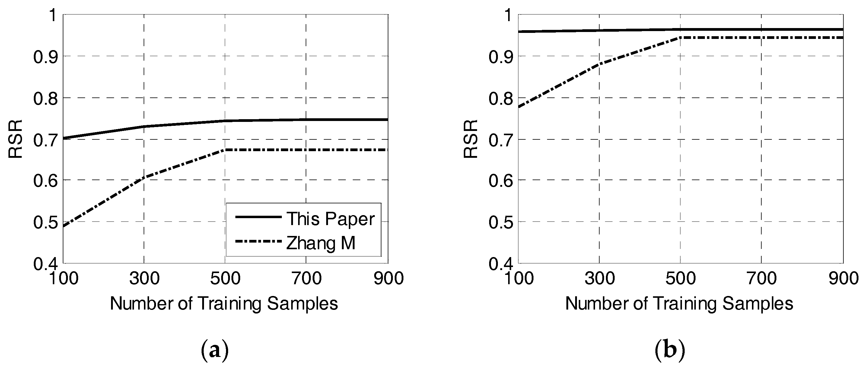
5.3. Experiment Results with Robustness

The following is to discuss the stability of system. The point is to ensure how recognition accuracy varies with the number of training samples. The training samples vary from 100 to 900 and the interval is 200. We draw the conclusions by comparing with Zhang’s [8] at SNR of −8 dB and −2 dB.

As Figure 11 shows, the recognition rates of this paper and Zhang’s are both increasing when the training data is from 100 to 900. The RSR of this paper is higher than Zhang’s under any training samples. When the number of training samples is 500, RSR is basically unchanged. That means the two systems are both stable at this time. When SNR is −8 dB, the growth of RSR is 18.5% for Zhang’s and the growth of this paper is 4.4%. When SNR is −2 dB, the growth of Zhang’s is 16.9% and the growth of this paper is only 0.7%. That means the growth of this paper is smaller than Zhang system. Therefore, the system of this paper has better robustness.

5.4. Experiment Results with Time

In order to measure the property of system, we calculate runtime to represent the computational complexity. Eight waveforms are tested when SNR is −8 dB and −2 dB. The simulation is repeated ten times and take the average. The time of this paper, Lunden’s [7] and Zhang’s [8] is shown in

Table 6. The time of this paper, Zhang’s and Lunden’s.

		BPSK	Costas	LFM	P1	P2	P3	P4	Frank
−8 dB	This paper	50.773	52.523	51.762	51.681	52.990	51.230	52.733	52.580
	Zhang	51.332	54.875	55.604	58.628	56.754	58.830	54.895	56.336
	Lunden	82.374	84.279	86.324	88.282	88.360	87.798	85.999	87.022
−2 dB	This paper	49.688	50.193	50.236	50.586	51.969	50.779	51.012	50.251
	Zhang	51.195	54.009	54.979	58.422	55.801	58.107	54.428	56.294
	Lunden	81.560	84.183	86.111	87.923	88.180	87.353	85.187	86.654

and the unit is seconds. The operation environment is in

Table 7. The operation environment.

Item	Version
CPU	E5-1620V2 (Intel)
Memory	16 GB (DDR3@1600 MHz)
GPU	NVS315 (Quadro)
MATLAB	R2012a

.

In order to make the data in Table 6 more clearly, the ratio of system’s (this paper and Zhang) time to Lunden’s time is calculated. The results can be seen in

Table 8. The ratio of system’s (this paper and Zhang) time to Lunden’s time.

		BPSK	Costas	LFM	P1	P2	P3	P4	Frank
−8dB	This paper/Lunden	0.616	0.623	0.599	0.585	0.599	0.583	0.613	0.604
	Zhang/Lunden	0.623	0.651	0.644	0.664	0.642	0.670	0.638	0.647
−2dB	This paper/Lunden	0.609	0.596	0.583	0.575	0.589	0.581	0.598	0.579
	Zhang/Lunden	0.627	0.641	0.638	0.664	0.632	0.665	0.638	0.649

.

As Table 8 shows, this paper’s time is about 0.595 of Lunden’s. Zhang’s time is about 0.645 of Lunden’s. That means the time of this paper is the least and the time of Lunden’s is the most. In Lunden system, some methods spend a lot of time but they are not utilized in this article. For example, data driven and peak search and so forth. In Zhang system, the number of features is 23 and there are only 14 features in this article. Therefore, the computational complexity of this paper is less than Zhang’s and Lunden’s.

6. Conclusions

In this paper, the system for recognizing 8 LPI radar waveforms is explored. The identifiable waveforms are BPSK, Costas codes, LFM, P1–P4 and Frank codes. There are only 14 features in the system and they are divided into time features and T-F features. Time features are obtained from the time domain signals. T-F features are related to the WVD and CWD and 3 new T-F features are proposed. The classifier of the system is SVM based on ABC algorithm. ABC is adopted to optimize the parameters of SVM and it can avoid the problem of local optimal solution to some extent.

The system has good performance and the details are as follows: Firstly, it has high recognition rate. When SNR at −4 dB, the overall RSR is 92% and the RSR of each waveform is all over 84%. Especially for LFM and P2 code, the RSR is about 97% which is far better than other systems. Secondly, it shows well robustness. When the training data is reduced to 100, the recognition rate is only dropped by 0.7% at SNR of −2 dB. Lastly, it possesses excellent computational complexity. The runtime of this paper is far less than other methods.

References

- Wang, S.; Zhang, D.; Bi, D.; Xue, D.; Yong, X. Research on recognizing the radar signal using the bispectrum cascade feature. J. Xidian Univ. 2012, 39, 127–132. [Google Scholar]
- Lopez-Risueno, G.; Grajal, J. Multiple signal detection and estimation using atomic decomposition and EM. IEEE Trans. Aerosp. Electron. Syst. 2006, 42, 84–102. [Google Scholar] [CrossRef]
- Wang, L.; Zhao, G. An Automatic Recognition Method for the Noise Frequency Modulation Signal. Electron. Sci. Technol. 2009, 22, 20–22. [Google Scholar]
- Wei, Y. A Detection Method for Noise Frequency Modulation Signal Bsased on Energy Statistics. Electron. Sci. Technol. 2010, 11, 020. [Google Scholar]
- Wang, X.; Zhou, Y.; Zhou, D.; Chen, Z.; Tian, Y. Research on Low Probability of Intercept Radar Signal Recognition Using Deep Belief Network and Bispectra Diagonal Slice. J. Electron. Inf. Technol. 2016, 38, 2972–2976. [Google Scholar]
- Ma, J.; Huang, G.; Zuo, W.; Wu, X.; Gao, J. Robust radar waveform recognition algorithm based on random projections and sparse classification. IET Radar Sonar Navig. 2014, 8, 290–296. [Google Scholar] [CrossRef]
- Lunden, J.; Koivunen, V. Automatic Radar Waveform Recognition. IEEE J. Sel. Top. Signal Process. 2007, 1, 124–136. [Google Scholar] [CrossRef]
- Zhang, M.; Liu, L.; Diao, M. LPI Radar Waveform Recognition Based on Time-Frequency Distribution. Sensors 2016, 16, 1682. [Google Scholar] [CrossRef] [PubMed]
- Vapnik, V. The Nature of Statistical Learning Theory; Springer: Berlin, Germany, 1995; pp. 988–999. [Google Scholar]
- Chang, C.C.; Lin, C.J. LIBSVM: A library for support vector machines. ACM Trans. Intell. Syst. Technol. 2011, 2, 27. [Google Scholar] [CrossRef]
- Cherkassky, V.; Ma, Y. Practical selection of SVM parameters and noise estimation for SVM regression. Neural Netw. 2004, 17, 113–126. [Google Scholar] [CrossRef]
- Shao, J.; Liu, J.H.; Qiao, X.G.; Jia, Z.A. Temperature compensation of FBG sensor based on support vector machine. J. Optoelectron. Laser 2010, 21, 803–807. [Google Scholar]
- Karaboga, D. An Idea Based on Honey Bee Swarm for Numerical Optimization; Erciyes University: Kayseri, Turkey, 2005. [Google Scholar]
- Brajevic, I. Crossover-Based Artificial Bee Colony Algorithm for Constrained Optimization Problems; Springer: Berlin, Germany, 2015. [Google Scholar]
- Zhu, Z.; Aslam, M.W.; Nandi, A.K. Genetic algorithm optimized distribution sampling test for M-QAM modulation classification. Signal Process. 2014, 94, 264–277. [Google Scholar] [CrossRef]
- Ozen, A.; Ozturk, C. A Novel Modulation Recognition Technique Based on Artificial Bee Colony Algorithm in the Presence of Multipath Fading Channels. In Proceedings of the 36th International Conference on Telecommunications and Signal Processing, Rome, Italy, 2–4 July 2013; pp. 239–243. [Google Scholar]
- Wong, M.L.D.; Nandi, A.K. Automatic digital modulation recognition using artificial neural network and genetic algorithm. Signal Process. 2004, 84, 351–365. [Google Scholar] [CrossRef]
- Wigner, E. On the Quantum Correction for Thermodynamic Equilibrium. Phys. Rev. 1932, 40, 749–759. [Google Scholar] [CrossRef]
- Cohen, L. Time-frequency analysis: Theory and applications. J. Acoust. Soc. Am. 1995, 134, 4002. [Google Scholar] [CrossRef]
- Hou, W.; Ou, G.; Chen, L.; He, Y. A simulation fast algorithm for parameters estimation of the multicomponent LFM signals. J. Chongqing Univ. Posts Telecommun. 2013, 12, 4385–4389. [Google Scholar]
- Meng, X.; Du, W.; Gao, X.; Shi, C. Research on identifying method of the Wigner-Ville distribution to crossing item. J. Naval Aeronaut. Eng. Inst. 2006, 1, 024. [Google Scholar]
- Jiang, L. Study on the Parameter Estimation of LPI Radar Signals of LFM Class. Ph.D. Thesis, Xidian University, Xi’an, China, 2016. [Google Scholar]
- Feng, Z.; Liang, M.; Chu, F. Recent advances in time–frequency analysis methods for machinery fault diagnosis: A review with application examples. Mech. Syst. Signal Process. 2013, 38, 165–205. [Google Scholar] [CrossRef]
- Pace, P.E. Detecting and classifying low probability of intercept radar; Artech House Inc.: Norwood, MA, USA, 2003. [Google Scholar]
- Gonzalez, R.C. Digital Image Processing; Pearson Education: Delhi, India, 2009. [Google Scholar]
- Fielding, J.E. Polytime coding as a means of pulse compression. IEEE Trans. Aerosp. Electron. Syst. 1999, 35, 716–721. [Google Scholar] [CrossRef]
Figure 1.
The structure of classification system is displayed in this figure. It is formed by time features, T-F features and classifier.
Figure 2.
The classifier is displayed in this figure. It includes two parts, i.e., network1 and network2.
Figure 3.
This figure shows the support vector machine (SVM) about two classes and linear separable problems. Margin means the geometric interval.
Figure 4.
In this figure, (a), (c) and (e) are the minimum and minimum values of Wigner-Ville distribution (WVD) of linear frequency modulation (LFM), Frank and P3 at signal to noise ratio (SNR) = 6 dB, respectively. (b), (d) and (f) are the absolute of the ratio of minimum to maximum of LFM, Frank and P3, respectively. There are 500 signals of each waveform.
Figure 5.
In this figure, (a) is the ratio of LFM, Frank and P3 at SNR = 6 dB; (b) is the ratio at SNR = −4 dB.
Figure 6.
The Choi-Williams distribution (CWD) results of eight waveforms are displayed in this figure. is set to 1 in this paper. (a) CWD image of LFM, (b) CWD image of Costas, (c) CWD image of BPSK, (d) CWD image of Frank, (e) CWD image of P1, (f) CWD image of P2, (g) CWD image of P3, (h) CWD image of P4.
Figure 7.
The procedure of transforming the resized image into binary image is displayed in this paper.
Figure 8.
CWD image processing of P4 code at SNR of −6 dB.
Figure 9.
In this figure, (a) and (b) are the framework of the maximum domain and its linear tendency of P4 and P1. (c) and (d) are the of P4 and P1. (e) and (f) are the of the two waveforms.
Figure 10.
Recognition accuracy at different SNR of each waveform. The overall RSR is 92% at SNR of −4 dB for this paper. (a) The RSR of BPSK (b) The RSR of Costas, (c) The RSR of LFM, (d) The RSR of P1, (e) The RSR of P2, (f) The RSR of P3, (g) The RSR of P4, (h) The RSR of Frank, (i) The overall RSR.
Figure 11.
In this figure, (a) is the RSR at different training samples at SNR = −8 dB. (b) is the result at SNR = −2 dB.