A Clustering Algorithm for Heterogeneous Wireless Sensor Networks Based on Solar Energy Supply


1
College of Computer, Nanjing University of Posts and Telecommunications, Nanjing 210003, China
2
Jiangsu High Technology Research Key Laboratory for Wireless Sensor Networks, Nanjing University of Posts and Telecommunications, Nanjing 210003, China
*
Author to whom correspondence should be addressed.
Electronics 2018, 7(7), 103; https://doi.org/10.3390/electronics7070103
Submission received: 3 June 2018
/
Revised: 21 June 2018
/
Accepted: 26 June 2018
/
Published: 28 June 2018
Abstract
:Limited battery power directly affects the performance and survival time of sensor networks. In this study, solar energy was used to provide additional energy for sensor nodes, and a clustering algorithm for heterogeneous wireless sensor networks (WSNs) based on a solar energy supply is proposed. A cluster head is selected on the basis of the self-replenishment state and the remaining energy of the nodes. A cluster-head selection mechanism and network layer multi-hop routing are adopted to balance the energy consumption of the network. A set of experiments showed that the proposed algorithm can effectively prolong the network lifetime, improve the stability and efficiency of the network, and balance the energy consumption compared with other algorithms under the same environmental energy supply.
1. Introduction
A wireless sensor network (WSN) is a distributed sensing network that is composed of sensor nodes that can perceive and detect the external world [1,2]. In WSNs, sensor nodes form multi-hop networks through wireless communication. The nodes around the base station perform their own data collection tasks and transmit the data sent by peripheral nodes. Thus, the energy consumption of these nodes is fast. The nodes far away from the base station consume more energy as a result of long-distance data transmission. The nodes in a traditional sensor network are powered by batteries, and the energy supply is limited. A large amount of energy consumption leads to energy depletion of nodes, which affects the lifetime of the network [3].
Networks are frequently clustered for energy consumption optimization to avoid rapid and irregular energy consumption to a certain extent. In WSNs, sensor nodes provide data reception and forwarding services to adjacent nodes by using a self-organizing network topology. A network cluster structure can be used to divide nodes and assign tasks to utilize the energy of the nodes and extend the lifetime of the WSN. However, these measures only reduce the energy consumption and cannot fundamentally solve the problem of battery energy limitation. Energy limitation is still one of the main obstacles for the practical application of WSNs [4,5,6].
Most of the current sensor nodes deployed still use batteries with limited energy as the energy sources in WSNs. With the continuous improvement of energy collection technology, solar, thermal, and mechanical vibrations in the surrounding environment have been converted into available electricity to supply sensor nodes [7]. However, the current technology for obtaining energy from the environment is unstable. The efficiency of energy harvesting largely depends on the surrounding environment, and the efficiency of energy harvesting is also different at different times [8,9]. Therefore, the energy collection technology cannot solve the energy consumption problem for sensor nodes and should be combined with an energy consumption optimization algorithm to achieve the continuous work requirements of networks [10,11].
Several clustering routing algorithms have been proposed to balance the energy consumption and prolong the lifetime of networks. The low-energy adaptive clustering hierarchy (LEACH) algorithm [12] is a classical clustering routing algorithm that assumes that all nodes in the network have the same structure and energy and that the nodes have no energy supply function. The distributed energy-efficient clustering (DEEC) [13] and stable election protocol (SEP) algorithms [14] assume that nodes have different initial energies and do not consider the energy recharge of nodes. The power-harvesting clustering (PHC) algorithm [15] investigates the clustering method of isomorphic WSNs with an energy supply, and the heterogeneous network includes self-Supplying Nodes (HNS) algorithm [16] evaluates the clustering method of heterogeneous WSNs with an energy supply.
In practical applications, heterogeneous sensor networks composed of different functional structure nodes exist widely. Most of the existing clustering routing algorithms are based on isomorphic networks. Few studies have reported on clustering routing algorithms for heterogeneous sensor networks that have advanced nodes with an energy supply and ordinary nodes without an energy supply. The hypothetical network used in this study uses advanced and ordinary nodes.
In this paper, a clustering algorithm for heterogeneous sensor networks based on a solar energy supply (CHSES) is proposed. In the cluster-head selection phase, the hibernation threshold of advanced nodes is set on the basis of the residual energy and energy self-recharge state of the nodes, and different thresholds are allocated for advanced nodes with a solar energy supply and ordinary nodes without a solar energy supply. This process increases the probability of high-level nodes being selected for the cluster head. In the data-transmission phase, a node is layered on the basis of the distance between the base station and the node. The nodes in the network are divided into clusters on the basis of the shortest-path principle, and the data are transmitted by combining information fusion and inter-layer multi-hop transmission. Thus, the network energy consumption is optimized, and the network lifetime is prolonged.
The remainder of this paper is organized as follows. Section 2 discusses some previous works on clustering algorithms that motivated our work. Section 3 presents the network and solar energy collection models in detail. Section 4 depicts the proposed algorithm. Section 5 presents the experimental simulation and algorithm evaluation. Finally, conclusions and future work are given in Section 6.
2. Related Work
In this section, we first introduce the existing clustering algorithms and then summarize the shortcomings of these algorithms.
2.1. Clustering Routing Algorithms without Energy Supply
2.1.1. LEACH Algorithm
The LEACH algorithm is a classic adaptive topology algorithm, the basic concept of which is to randomly select cluster-head nodes and consistently distribute the entire network energy load to individual sensor nodes in the network, which reduces the network energy consumption and improves the network lifetime.
The execution of the algorithm is periodic, and the reconfiguration of clusters is continuously executed. The operation of the algorithm adopts the concept of “rounds”, and each round consists of two stages, namely, initialization and stabilization. In the initialization stage, each node generates a random number between 0 and 1. The node delivers itself as the cluster head’s message, and neighboring nodes join the cluster on the basis of the shortest-path principle when the node’s random number is less than or equal to the threshold. In the stable stage, the cluster nodes send data to cluster heads; meanwhile, the cluster heads perform data fusion and send the fusion information to the base stations. The energy consumption is large because cluster heads require data fusion and communication with base stations. The LEACH algorithm can guarantee that the probabilities of each node being the cluster head are virtually equal and that the nodes consume energy in a relatively balanced manner.
In the LEACH algorithm, each cycle is required to reorganize the cluster, and the energy cost of the cluster is large. The cluster-head nodes far away from the base stations may consume energy in advance as a result of long-distance transmission, which results in unbalanced network energy consumption and a shortened overall lifetime. In addition, the LEACH algorithm does not consider the current energy state of cluster-head nodes. The death of nodes is accelerated, and the lifetime of the entire network is affected when low-energy nodes are used as cluster heads.
2.1.2. DEEC Algorithm
The LEACH algorithm assumes that a network is isomorphic. However, in the true situation, the nodes in the sensor network are often heterogeneous because of their different geographical location distributions, performance, and other factors.
The DEEC algorithm is a routing algorithm that is applied for multi-level energy-heterogeneous networks. The multi-level energy-heterogeneous representation indicates that the initial energy of nodes can take on many different values. In DEEC, the probability for a node to be defined as a cluster head is based on the ratio of the current residual energy of the node to the average energy of the network. The energy consumption can be effectively balanced and the network lifetime can be extended by considering the residual energy of the node. However, DEEC uses an estimation scheme to solve the network average residual energy in which the network energy consumption is uniform, which is inconsistent with reality and weakens the practicability of DEEC.
2.1.3. SEP Algorithm
The SEP algorithm is applied on clustered networks with heterogeneous energy. The SEP describes the influence of energy isomerism on heterogeneous perception and instability. The algorithm includes advanced and ordinary nodes. Advanced nodes have high initial energy and are set to of the ordinary nodes. On the basis of the initial energy of the nodes, an election probability factor is configured for each node to determine its probability as cluster head and to achieve uniform energy consumption.
However, in SEP, the election probability is only related to the initial energy of the node and not to the current remaining energy. The number of advanced nodes to be selected as the cluster is more than that of the ordinary nodes, and the energy of an advanced node may be lower than that of an ordinary node after a certain cycle.
2.2. Clustering Routing Algorithms with Energy Supply
2.2.1. PHC Algorithm
The PHC algorithm is a clustering routing algorithm with energy replenishment. In the cluster-formation stage, the PHC algorithm improves the existing cluster-head selection and non-cluster-head attribution mechanisms under the consideration of energy supply, and it is similar to LEACH in the data-transmission phase.
To avoid the selection of low-energy nodes as cluster heads, PHC improves the existing cluster-head selection mechanism on the basis of the energy supply and energy level of the nodes. The PHC algorithm modifies the threshold of selected nodes as cluster heads. The threshold is related to the energy supply of the nodes on the basis of their current energy level, which increases the probability of nodes with a high energy level being selected and decreases the probability for nodes with a low energy level.
2.2.2. EBCS Algorithm
The energy-balanced clustering with self-energization (EBCS) algorithm is a type of energy-balanced clustering routing algorithm used in WSNs. Considering the different amounts of recharge energy obtained from the nodes in different geographic regions, the EBCS algorithm combines the characteristics of the true energy supply to improve the selection mechanism of the cluster head and considers the residual energy of the node and the total recharge energy of the node starting from the last turn to be the cluster head to the recent rotation. An inter-cluster communication mechanism is used to achieve the complete reduction and utilization of recharge energy.
However, a smaller cluster head exists in the energy-surplus phase when all nodes participate in the cluster-head selection mechanism. No special protection measures are reported to prevent the selection of nodes with low energy as the cluster head.
2.2.3. HNS Algorithm
The HNS algorithm is a heterogeneous sensor network clustering routing algorithm with energy self-replenishing nodes that uses vibration energy as an energy supplement. In the cluster-head selection, HNS assigns different thresholds to the nodes with different functions. HNS considers the residual energy and current energy supply state of the nodes at the same time to select cluster heads. In the multi-hop area, the shortest path is adopted on the basis of the distance from the convergence node.
An advanced-node state-transition model has been designed that enables advanced nodes to adjust the transformation state on the basis of the remaining energy. The states of nodes consist of active, energy-storage, and dormancy periods, and nodes in different stages have different functions. The algorithm also improves the cluster-head selection mechanism on the basis of the residual energy and energy self-replenishment state of the nodes. Ordinary and advanced nodes are separately discussed when the cluster head is selected, and the energy self-recharge-state coefficient is designed to make the nodes with a better supply state obtain a higher cluster-head selection probability and balance the network consumption.
2.3. Problem Analysis
After analysis, the above clustering routing algorithms still have the following shortcomings.
- (1)
- The traditional clustering routing algorithm does not consider that a node has an additional energy supply. The selection probability is only related to the initial energy of the node and does not consider the remaining energy. An advanced node is more likely to be selected as the cluster head than an ordinary node. After a certain number of rounds, the energy of an advanced node may be lower than that of an ordinary node, which increases the network energy consumption and accelerates the decline of the network.
- (2)
- The PHC [15] and EBCS algorithms [17] assume that the energy self-recharge of the nodes is steady and uninterrupted. In the true situation, the nodes cannot constantly obtain the same acquisition efficiency because of the irregular distribution of the energy supply in each region. This condition causes the cluster head to be mainly concentrated in the region with a high current energy supply level; the number of cluster heads in the area with a low energy supply is small, and the members are excessive in the cluster. Several clusters cause the overloading of cluster heads and affect the average residual energy and lifetime of the network.
- (3)
- The HNS algorithm [16] sets the node energy self-replenishment-state coefficient to increase the probability for nodes with a better energy self-replenishment status to be selected as cluster heads. However, the algorithm ignores the nodes with slow energy-storage efficiency and accumulates high residual energy through several rounds, which causes the excessive loading of several nodes with high energy-storage efficiency, makes the network energy consumption unbalanced, and affects the network stability.
Considering the above problems, this study proposes a heterogeneous sensor network clustering routing algorithm called CHSES that contains energy recharge. The innovative points of this algorithm are expressed as follows:
- (1)
- Energy classification is used to set different initial energies for advanced and ordinary nodes to increase the probability of high-level nodes to serve as cluster heads. Meanwhile, a hibernation threshold is set for the advanced nodes to enable advanced nodes with an energy lower than the threshold value to only store energy and to prevent them from participating in the cluster-head competition that prolongs the lifetime of the network.
- (2)
- The algorithm increases the influence factor of residual energy. Meanwhile, the nodes with high residual energy and a better energy supply state have a high probability to be selected as cluster heads, and the influence of energy self-recharge parameters on the threshold of the node cluster head is gradually weakened. The nodes that have slow energy-storage efficiency and high residual energy can also be selected as cluster heads over several rounds to increase the number of cluster heads as far as possible and avoid the overloading of cluster heads.
- (3)
- Nodes are layered and use multi-hop transmission on the basis of the distance between the node and the base station. The network is layered to increase the probability of the inner network node becoming the cluster head. The cluster head of the outer layer passes the data packet to the advanced node that is high and near to it and does not directly transmit data to the base station, which avoids energy loss caused by long-distance transmission.
3. Model Construction
3.1. Heterogeneous Sensor Network Model
N sensor nodes are randomly distributed in a monitoring area. They monitor and send data periodically. The assumptions are expressed as follows:
- (1)
- The network is composed of a small number of advanced nodes and a majority of ordinary nodes. An advanced node has the energy self-replenishment function, and ordinary nodes only use a lithium battery to supply power.
- (2)
- The positions of the advanced and common nodes are fixed.
- (3)
- Nodes have their own independent ID, certain data storage, and fusion capabilities.
3.2. Wireless Communication Energy Consumption Model
The communication energy consumption model is adopted as for LEACH [12]. The distance threshold of the power amplifier is used in different situations. The power amplifier adopts the free-space model when the distance between the transmitter and receiver is less than ; the amplifier uses the multi-path attenuation model when the distance between the transmitter and receiver is greater than or equal to .
The energy consumed to transmit data to the destination node can be calculated as
where is the energy loss of the circuit; and are the energy factors of the power amplifier when the free-space and multi-path attenuation models are used, respectively; and l is the length of the sent data packet.
The energy consumed by nodes to receive and integrate data can be calculated as
where is the energy loss of the receiving circuit, is the energy loss of data fusion, and l is the length of the received data packet.
3.3. Energy Supply Model in Real Environment
Energy-harvesting nodes have the ability to harvest energy from the surrounding environment. Currently, energy-harvesting sensor nodes mainly use solar and vibration energies as energy sources. The power density of general solar power is approximately 10–15 mW/cm, and that of vibration energy is approximately 0.275 mW/cm [18,19]. Clearly, solar energy has a higher energy supply efficiency than vibration energy. Thus, we use solar energy as an additional energy supply in this paper. Because of the time and periodicity of solar harvesting, we discuss the model of solar energy harvesting in this section.
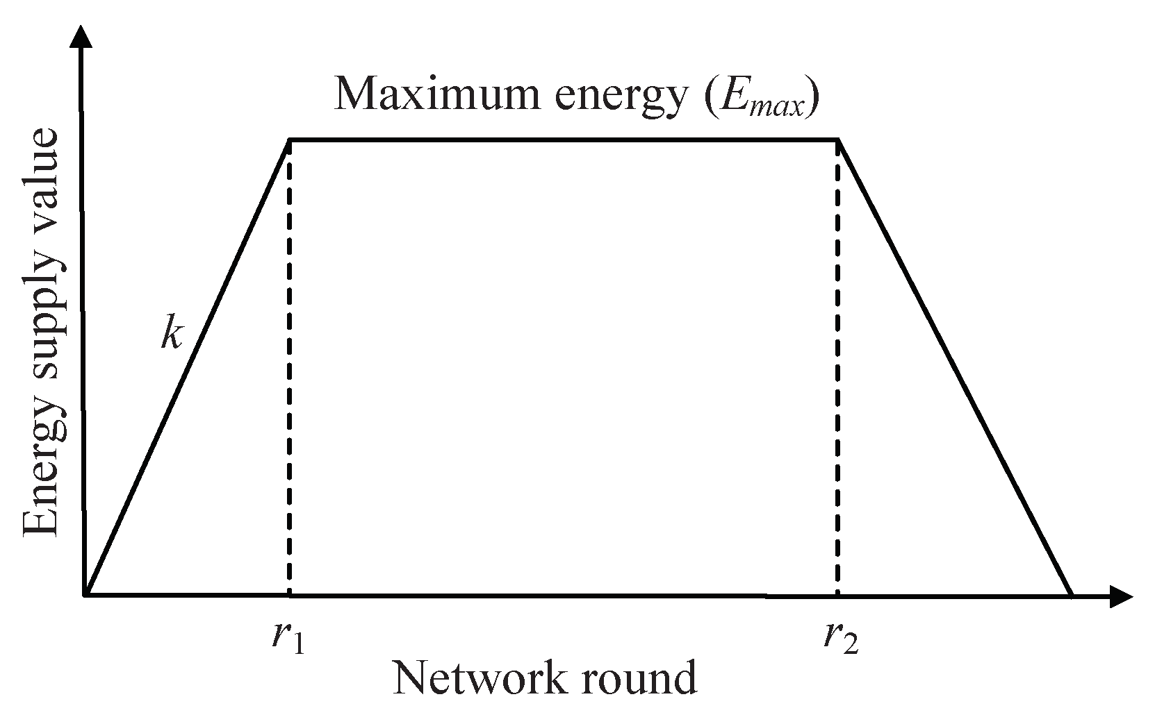
The trapezoidal model is a common model of solar energy supply. No sunlight or energy supply exist at night, and high solar light and maximum energy supply rates at noon are observed in one day. From sunrise to sunset, solar energy reaches its maximum daily supply with time and continues to decline after a certain period. Therefore, a basic solar energy model is established, as illustrated in Figure 1. The relationship between solar recharge and the number of rounds is expressed as follows:
where denotes the average level of nodes in round r of energy replenishment and is the maximum value for energy collection in a day. The amount of energy collection before round increases at rate k. The energy collection of the node between rounds and reaches the maximum and is maintained at this level for a period of time. The energy harvesting of nodes after round decreases at rate k and reaches zero.
The trapezoid model simulates the theoretical value of solar energy collection in a sunny day. However, in the true situation, nodes of different locations may be affected by external factors, such as possible shelter and different incident angles of the sun. The same node is also affected by factors such as weather and self-replenishment. The true situation for solar energy does not conform to the trapezoidal model.
In [20], solar radiation data were used to fit an empirical curve to obtain a high availability of the solar energy model. Solar energy collection data from 2005 to 2009 were used as the active solar energy, and the solar data model of 2010 was fitted. Thus, a single model was designed for each season in [20], because the annual solar intensity varied remarkably. The fitting results showed that the Gauss function and polynomial function were close to the true solar-collection situation, as shown in Figure 2.
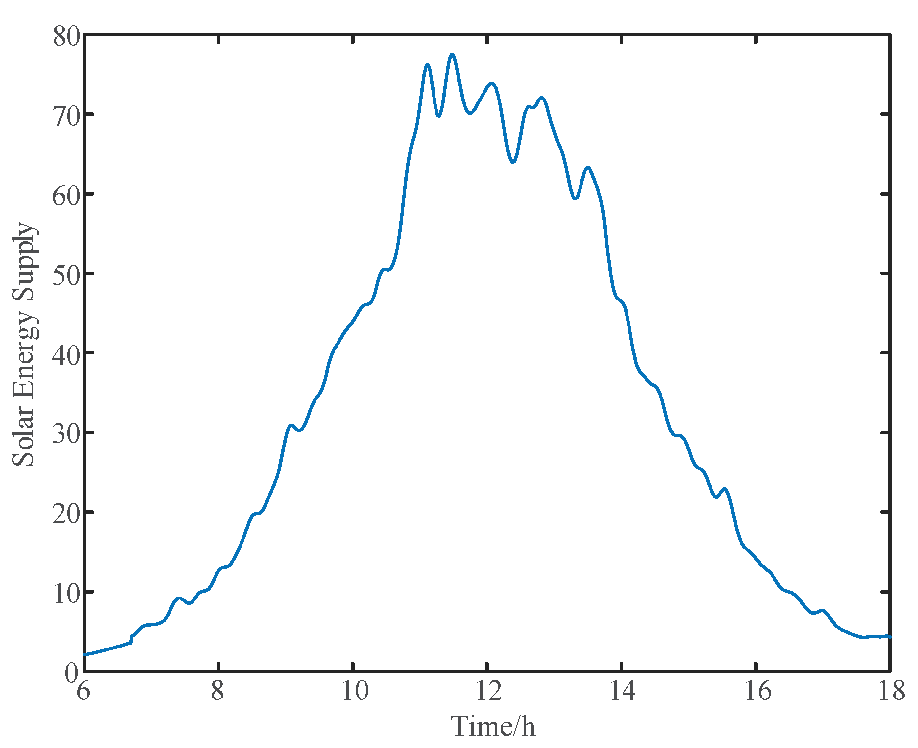
The Gaussian model is clearly better than the trapezoidal model for the true situation of daily solar energy collection, but several shortcomings still exist. In [21], the seasonal collection characteristics of solar energy were obtained through experimental analysis. In reality, the solar collection trend rises and falls. However, solar collection does not have a smooth curve because of weather changes. By contrast, solar collection is random. Figure 3 shows the true solar collection status of Oak Ridge on 9 March 2018 [22].
To better simulate solar energy collection, we use the Gaussian kernel density model to model energy harvesting. Kernel density estimation is a non-parametric method used to estimate unknown density functions in probability theory. The Gaussian kernel density function is a function generated by kernel density estimation for a normal distribution model. This function is defined by Equation (4):
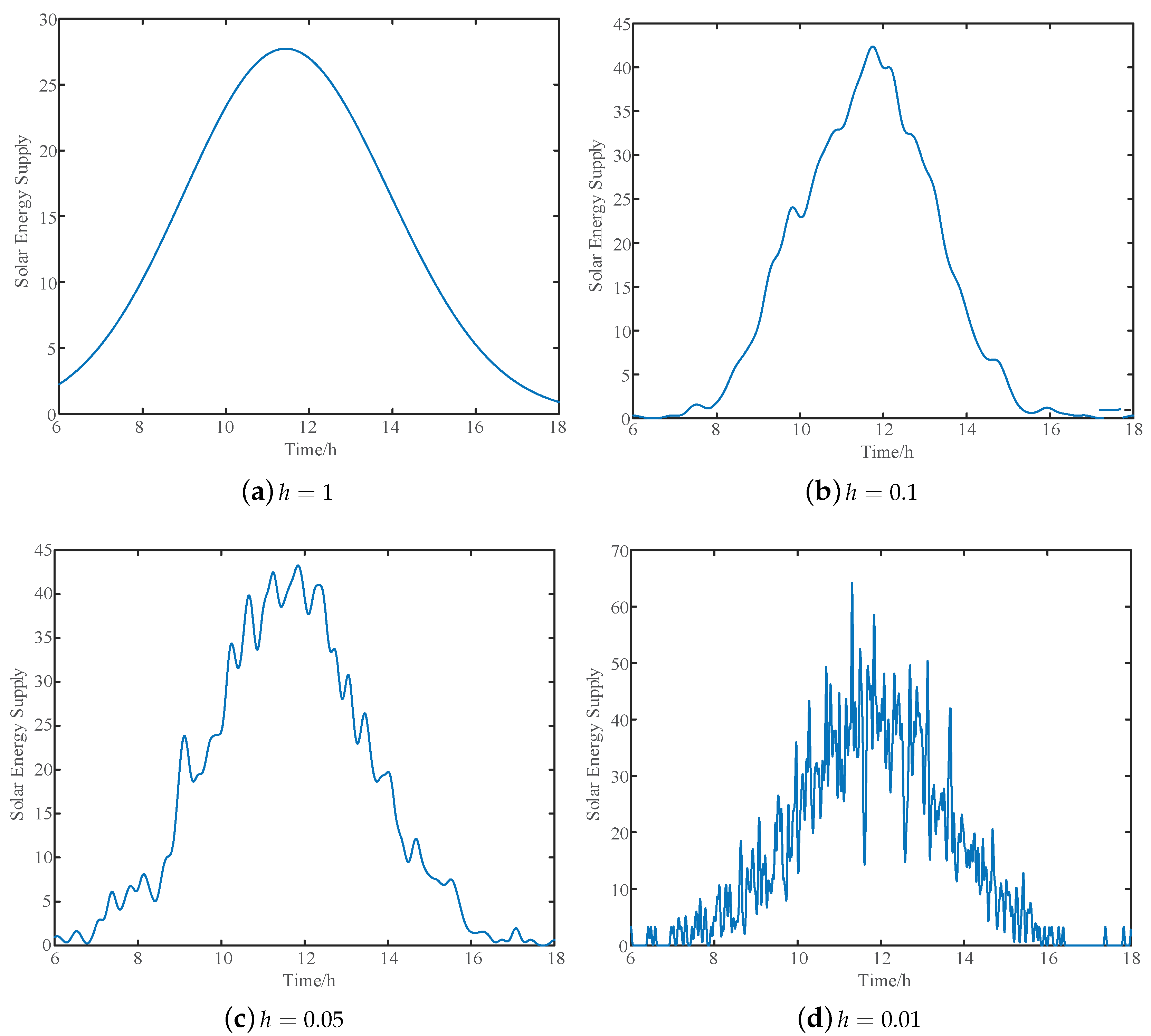
where , , are the random numbers for a group with a normal distribution, n is the number of random numbers, and h is the window width of the kernel density function. A change in the window width can change the steepness of the curve, as shown in Figure 4.
As shown in Figure 4, the solar energy recharge model built by the Gaussian kernel density function is stochastic. The model can simulate various basic weather conditions, such as sunny, cloudy, and rainy days, and can also simulate various complicated weather changes, such as the weather change from fine to cloudy.
Figure 5 shows the true weather situation simulated by the Gaussian kernel density model. The first half of the curve slowly increases, and fluctuations occur at irregular intervals, which is consistent with the true supply situation of solar energy in the morning. The central part of the curve is essentially maintained at the same level but with clear fluctuations. The solar collection reaches the highest value and remains for a time period, and the amount of solar energy also fluctuates as a result of small changes in the weather. The latter half of the curve steadily descends, which is in line with the declining trend of solar recharge in the afternoon.
Compared with the trapezoidal and Gaussian models, the Gaussian kernel density model is more general and closer to the true situation of solar recharge.
3.4. State-Transformation Model of Advanced Nodes
In heterogeneous WSNs, advanced nodes have a self-energy replenishment function. Each energy-harvesting node has an energy limit threshold. If the energy of an advanced node is less than this limit threshold, the node is automatically blocked, does not participate in the current round, and does not send data until the energy status reaches the desirable level. The sensor node is delivered from the block mode, turns to active mode, joins the network, and starts to send and receive data in the next round when its energy is higher than the limit threshold.
The mode transition parameter of an advanced node is set as follows:
where is the residual energy for sensor nodes and is the energy limit threshold. Advanced nodes enter the active mode and participate in the cluster-head competition when is equal to 1. An advanced node enters the block mode and only collects data and sends data packets when is equal to 0.
4. Algorithm Design
The proposed algorithm in this study can be divided into setup and data-transmission phases.
4.1. Setup Phase
In heterogeneous sensor networks, many advanced nodes should be selected as cluster heads to extend their lifetime as much as possible. The cluster-head selection mainly considers two factors: (1) The nodes with large residual energy or a considerable energy supply should be selected as cluster heads to undertake several data-forwarding tasks. (2) The proportion of the total number of cluster-head nodes in a network should be limited.
On the basis of the SEP and HNS algorithms, a heterogeneous sensor network clustering algorithm based on solar recharge is proposed in this section. The initial energy of the network node uses energy classification to set different initial energies for the advanced and ordinary nodes, which increases the probability of an advanced node serving as the cluster head. Advanced and ordinary nodes are separately discussed, and different electoral thresholds are set during the selection of cluster heads.
For an advanced node with an energy supply, the influence of residual energy and the energy self-recharge state on the threshold is increased on the basis of the traditional threshold setting. The algorithm compares the sum of residual and harvested energies with the low initial energy of the advanced node. Thus, a node that has considerable residual energy and a better self-recharge state has a high probability to be selected as the cluster head.
For ordinary nodes without energy recharge, the influence of residual energy is increased. The definition of different election thresholds is set as follows:
where p is the proportion of the ideal cluster head, r is the number of rounds, is the initial energy of the node, expresses the current residual energy of node i, represents the energy that the node has supplied from the last selected cluster to the present, and is the influence factor of the remaining energy that is defined as follows:
Equation (7) represents that is a general type of arithmetic progression. In the first round, . With an increase in the number of rounds, gradually decreases until round 1/p reaches 0; also gradually decreases from 1 to 0 when the new round begins. In this way, the proportion of in Equation (7) is weakened.
The probability of the nodes with poor energy-collecting efficiency but gradually accumulated considerable residual energy is improved when the nodes with good residual energy and a good energy supply state have a high probability to be selected as cluster heads. Thus, the number of cluster heads at the weak energy supply level is increased, and the overloading of cluster heads is avoided.
As shown in Equation (6), the cluster-head selection algorithm separates the advanced nodes from the ordinary nodes, improves the probability of the advanced nodes becoming the cluster head, reduces the energy consumption of the nodes, and balances the energy consumption of the network. For ordinary nodes, a node with high residual energy has a higher probability of becoming a cluster head by comparing the residual energy of the node with the original energy, which prolongs the lifetime of the node.
For advanced nodes, a node with high residual energy and a better energy supply state is selected as the cluster head by comparing the residual energy and harvesting energy of the nodes with the original energy, which ensures the high probability of nodes with high energy becoming the cluster head. The influence of the energy self-recharge state on the cluster-head selection is gradually weakened by increasing the influence factor of residual energy. Thus, the nodes with a poor energy supply state but gradually accumulated considerable residual energy can also become cluster heads, which shares the network load and balances the network energy consumption. The detailed steps of the setup phase are described in Algorithm 1.
| Algorithm 1: Setup phase of CHSES algorithm |
| 1) BEGIN; 2) while CT < TimePh1 do 3) if Sensor[i].state == ’Cluster Head’ then 4) Sensor[i].state = ’Node’; 5) endif 6) endwhile 7) while CT < TimePh2 do 8) if Sensor[i].property == ’Advanced’ then 9) if Sensor[i].energy > the block threshold then 10) predict node energy collection; 11) calculate the election threshold of Sensor[i] by Equation (6); 12) generate random numbers between 0 and 1; 13) if λ < the election threshold then 14) Sensor[i].state = ’Cluster Head’; 15) broadcast Head_Msg; 16) receive Head_Msg from competition Cluster Head; 17) store in Head_List Cluster Head L[] along with distance; 18) endif 19) endif 20) else if Sensor[i].energy < the block threshold then 21) block automatically and do not allow participation in the current round; 22) endif 23) endif 24) else if Sensor[i].property = ’Ordinary’ then 25) if Sensor[i].energy > 0 then 26) calculate the selection threshold of Sensor[i] by Equation (6); 27) generate random numbers between 0 and 1; 28) if λ < the election threshold then 29) Sensor[i].state = ’Cluster Head’; 30) broadcast Head_Msg; 31) receive Head_Msg from competition Cluster Head; 32) store in Head_List Cluster Head L[] along with distance; 33) endif 34) endif 35) else if Sensor[i].energy ⩽ 0 then 36) exit the network; 37) endif 38) endif 39) endwhile 40) while CT < TimePh3 do 41) if Sensor[i].state == ’Node’ then 42) select the nearest Cluster Head Sensor[j] from Cluster Head L[] list; 43) Sensor[i].head = Sensor[j]; 44) send Join Cluster Msg to Sensor[j]; 45) endif 46) else if Sensor[i].state == ’Cluster Head’ then 47) receive Join Cluster Msg from Cluster Member; 48) store in Cluster Member[] List; 49) endif 50) endwhile 51) END |
4.2. Data-Transmission Phase
In the data-transmission phase, the CHSES algorithm uses the first-order wireless communication energy consumption model [23] and calculates the energy consumption on the basis of the distance, as shown in Equation (1). The data between nodes are transmitted in the multi-hop mode, and energy consumption is closely related to path selection.
In this paper, we adopt a node hierarchical multi-hop transmission mechanism for data transmission. The hierarchy of the network is stratified on the basis of the distance between the nodes and the base station. The higher the node level, the higher the probability of the node becoming the cluster head. Thus, the number of nodes in the inner layer of the network is increased to avoid the premature death of nodes due to overloading. The cluster head of the outer layer passes the packet to the advanced node that is high and nearest to it on the basis of the shortest-path principle and does not directly transmit the data to the base station. Thus, the energy loss caused by the long-distance transmission of data is avoided.
After the end of each cluster-head selection, all nodes select the nearest cluster-head node to transmit data on the basis of the shortest-path principle. Cluster-head nodes receive all the data of member nodes in the cluster, compress and fuse the data, and enter the transmission stage.
We divide the nodes near the base station into two situations to avoid the overloading of nodes near the base station and the overloading of cluster heads. The distance from the node to the nearest cluster head is , and the distance from the node to the base station is . The node transfers the data packet to the cluster head when , and the cluster head fuses all the data packets to one data packet and transmit this to the base station. Conversely, the node directly communicates with the base station when . This process optimizes the network energy consumption and prolongs the network lifetime. The detailed steps of the data-transmission phase are described in Algorithm 2.
| Algorithm 2: Data-transmission phase of the CHSES algorithm |
| 1) BEGIN; 2) while CT < TimePh1 do 3) if Sensor[i].state == ’Cluster Head’ then 4) select the nearest advanced node Sensor[j] in higher Layer; 5) Sensor[i].next-hop = Sensor[j]; 6) endif 7) endwhile 8) while CT < TimePh2 do 9) if Sensor[i].state == ’Cluster Head’ then 10) receive Data Packet from Cluster Member; 11) aggregation of Data Packet; 12) broadcast Data Packet to base station or next hop; 13) endif 14) else if Sensor[i].state == ’Node’ then 15) broadcast Data Packet to Cluster Head; 14) endif 17) endwhile 18) END |
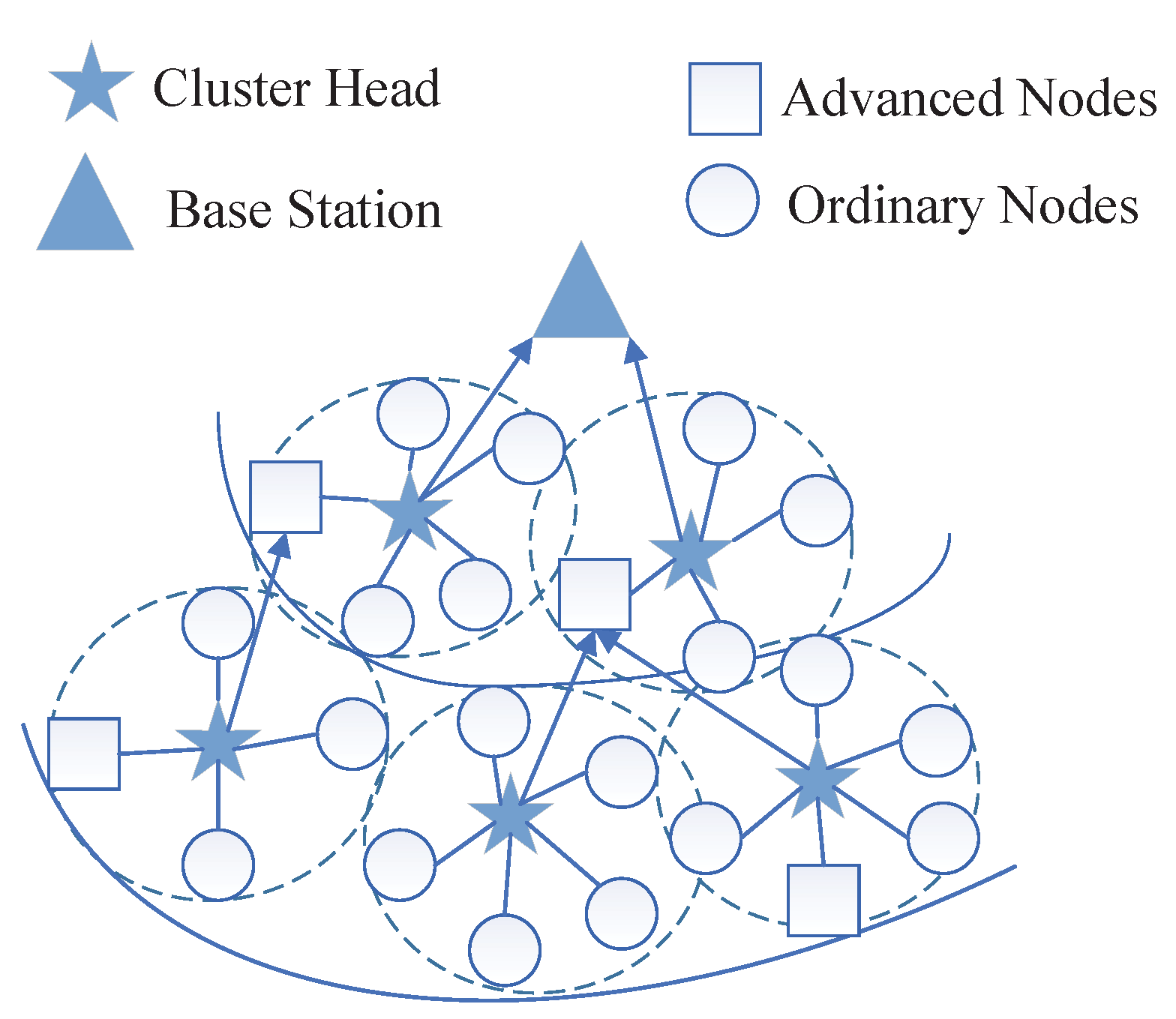
In conclusion, in the data-transmission phase, the large amount of energy consumption caused by the direct communication between the low-level nodes and base station is avoided. The topology diagram for the layered transmission of network nodes is illustrated in Figure 6. The cluster-head node selects the upper-level node on the next hop as the relay node, which utilizes the advanced-node energy self-replenishment. By contrast, the energy consumption speed of the nodes around the base station is reduced, and the lifetime of the nodes is prolonged by increasing the number of cluster heads in the inner layer of the network and selecting the shortest transmission principle of the inner node.
4.3. Algorithm Flow
The proposed clustering routing algorithm in this paper is iterative on the basis of the round. Each cycle includes the establishment of a cluster and data transmission in two stages, and the specific algorithm flow is represented in Figure 7.
At the stage of each cluster formation, the advanced node calculates the current residual energy, the energy recharge from the last selected cluster head to the current cluster head, and the residual-energy influence factor for the current round of the node. Thus, the selected threshold is calculated. The specific steps are as follows:
- (Step 1)
- The advanced node considers its own residual energy. The node enters the dormancy state, and the current round is temporarily out of the cluster-head competition if the residual energy E is less than ; the algorithm proceeds to step 4. Otherwise, step 2 is performed.
- (Step 2)
- Nodes generate a random number between 0 to 1. If is less than the threshold, then the node is selected as the cluster head, and step 3 is performed. Otherwise, the algorithm proceeds to step 4.
- (Step 3)
- Cluster-head nodes broadcast the cluster-head information and wait for non-cluster-head nodes to join.
- (Step 4)
- A node receives the broadcast information of the cluster-head node, calculates the path, selects the optimal-path node as the cluster head, sends the cluster request, and periodically collects the data to the cluster head.
- (Step 5)
- The cluster head receives the data from its own regular collection and receives the data sent by the member nodes in the cluster at the same time, compresses and fuses the data, and enters the data-transmission phase. Data are transmitted across the clusters by multi-hopping and reach the base station.
5. Evaluation and Simulation
5.1. Simulation Scene and Parameter Setting
The network simulation scenario was a square area of 100 × 100 m, and 100 nodes were randomly distributed in the network. The base station was fixed in the regional center, and the location coordinates were [50, 50].
The node energy-recharge model uses the solar energy model. In a real environment, the real-time acquisition rate of solar energy is markedly influenced by weather and has a certain randomness. To better simulate the true energy acquisition, we use the Gaussian kernel density solar energy model, as illustrated by Equation (4).
Under the same network environment, the values of the advanced-node state-transition model of the clustering routing algorithm were compared with different set values. The set values were changed from to . The average numbers of rounds until the first death of a node occurred under different settings are indicated in Table 1. The number of rounds until the first dead node occurred in the network was the greatest when was used. Thus, was set as 50% of the initial energy of the advanced node. Other parameters are listed in Table 2.
5.2. Simulation Results and Analysis
We used the LEACH [12], energy harvesting-LEACH (EH-LEACH), SEP [14], DEEC [13], PHC [15], and HNS [16] algorithms in MATLAB simulation software under the same rules of energy supply to conduct experiments on heterogeneous WSNs with energy acquisition nodes (20%). We compared and analyzed the performance differences between them and the proposed clustering algorithm through simulation in terms of the remaining number of surviving nodes, energy balance consumption, and other indicators.
5.2.1. Comparison of Network Lifetimes
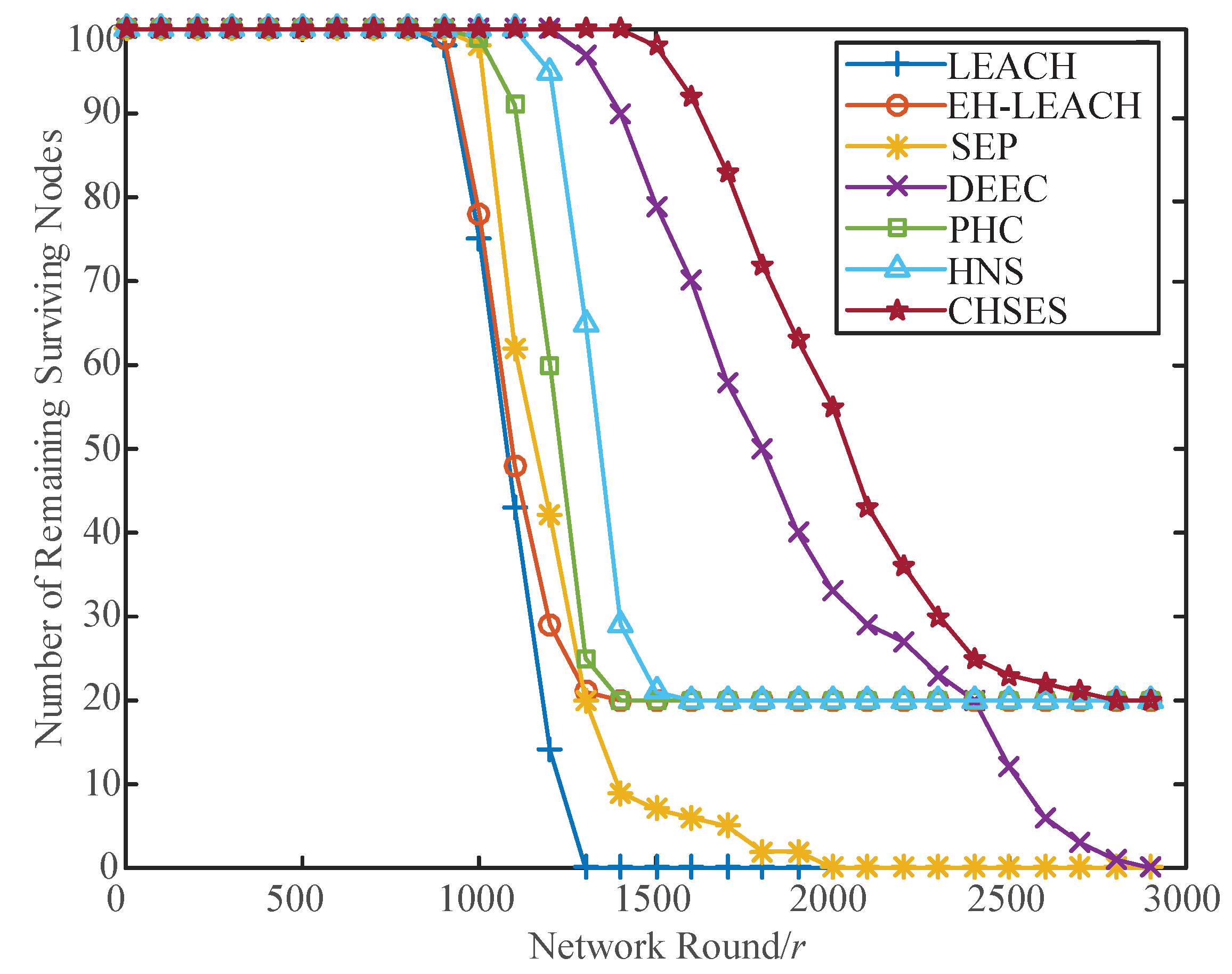
The average residual energy of the nodes using different algorithms decreased with the increase in the number of rounds. As shown in Figure 8, the number of remaining surviving nodes for the traditional LEACH and SEP algorithms was less than 20% at the 1500th round. Meanwhile, the EH-LEACH algorithm with energy supply and that uses the same energy supply rule was slower than the traditional LEACH algorithm in terms of the node death rate. However, the number of live nodes was less than half of the number of original nodes at the 1500th round.
As shown in the analysis in Figure 8 and Table 3, the network nodes that used the traditional LEACH algorithm all died in the 1362nd round, and the numbers of remaining surviving nodes of the PHC, HNS, and DEEC algorithms were 76, 81, and 96, respectively. The proposed clustering routing algorithm did not obtain the first dead node. This condition indicates that the clustering routing algorithm extends the network lifetime and increases the network stability.
5.2.2. Comparison of Network Stability Cycle
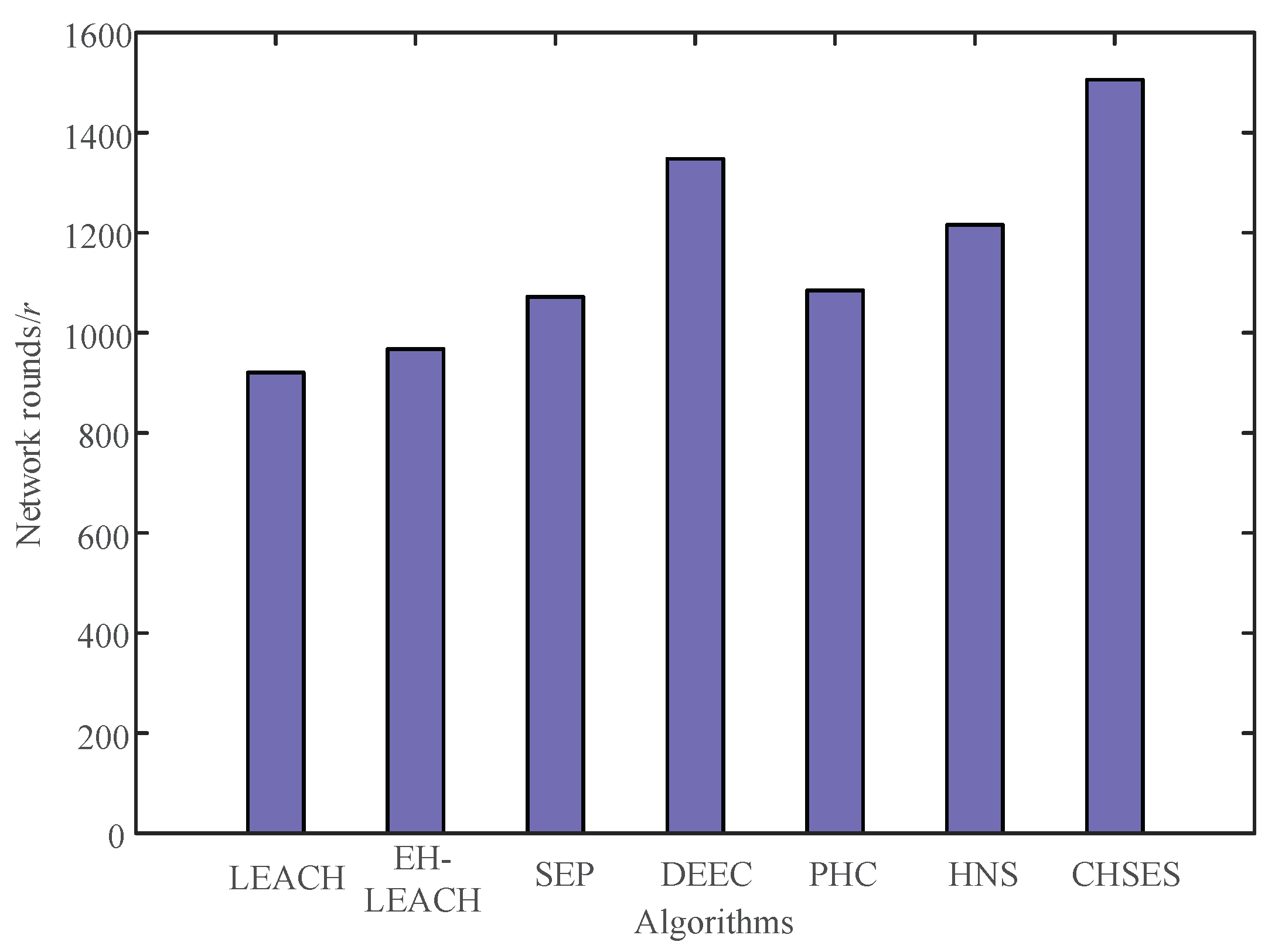
In WSNs, we usually call the start time from the initialization of the network to the death of the first node the “stable cycle” of the network. For a long period of time, the stable cycle is important to ensure the normal operation of the entire network and efficient data transmission. As shown in Figure 9, the stability period of the proposed clustering routing algorithm was the longest, and the number of round before the first dead node was 1506, which makes the algorithm clearly superior to the others.
5.2.3. Comparison of Network Energy Consumption Balance
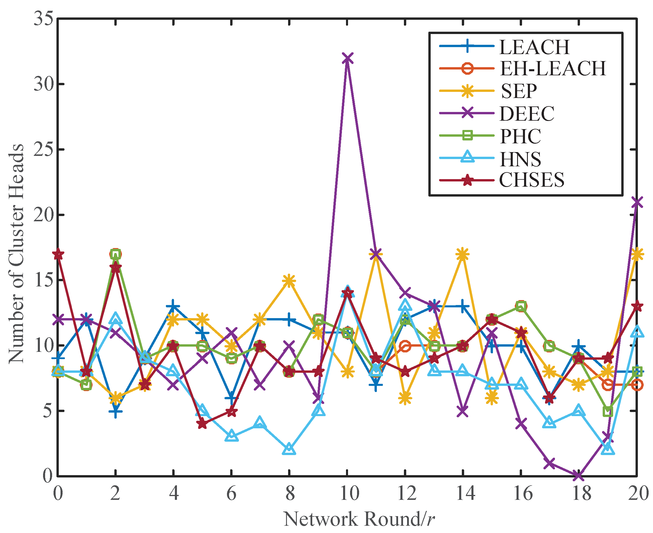
To optimize network performance, the proportion of cluster heads to the total number of nodes in the network should be controlled. In the simulation, we set the ideal cluster-head ratio of p to 0.1; that is, the number of selected cluster heads in every round of the network was approximately 10. On the basis of the analysis of the first two items, the proposed clustering routing algorithm was clearly better than the other algorithms in terms of the survival of the remaining nodes and the network stability period. The following is for the DEEC algorithm.
As illustrated in Figure 10, the cluster-head number of each cluster for the proposed clustering routing algorithm was between 5 and 15, which was essentially the same as was expected. In the 11th round of the DEEC algorithm, the number of cluster heads exceeded 30, and it dropped to 0 in the 19th round. Although the cluster-head selection has a certain randomness, the immense change in cluster-head number is clearly not conducive to the long-term stability of the network, particularly in the case of an uneven distribution of the network. It was easy to observe the heavy load of some nodes and the shortening of the lifetime of the nodes, as well as the effects on the energy consumption of the network.
5.2.4. Comparison of Network Residual Energy
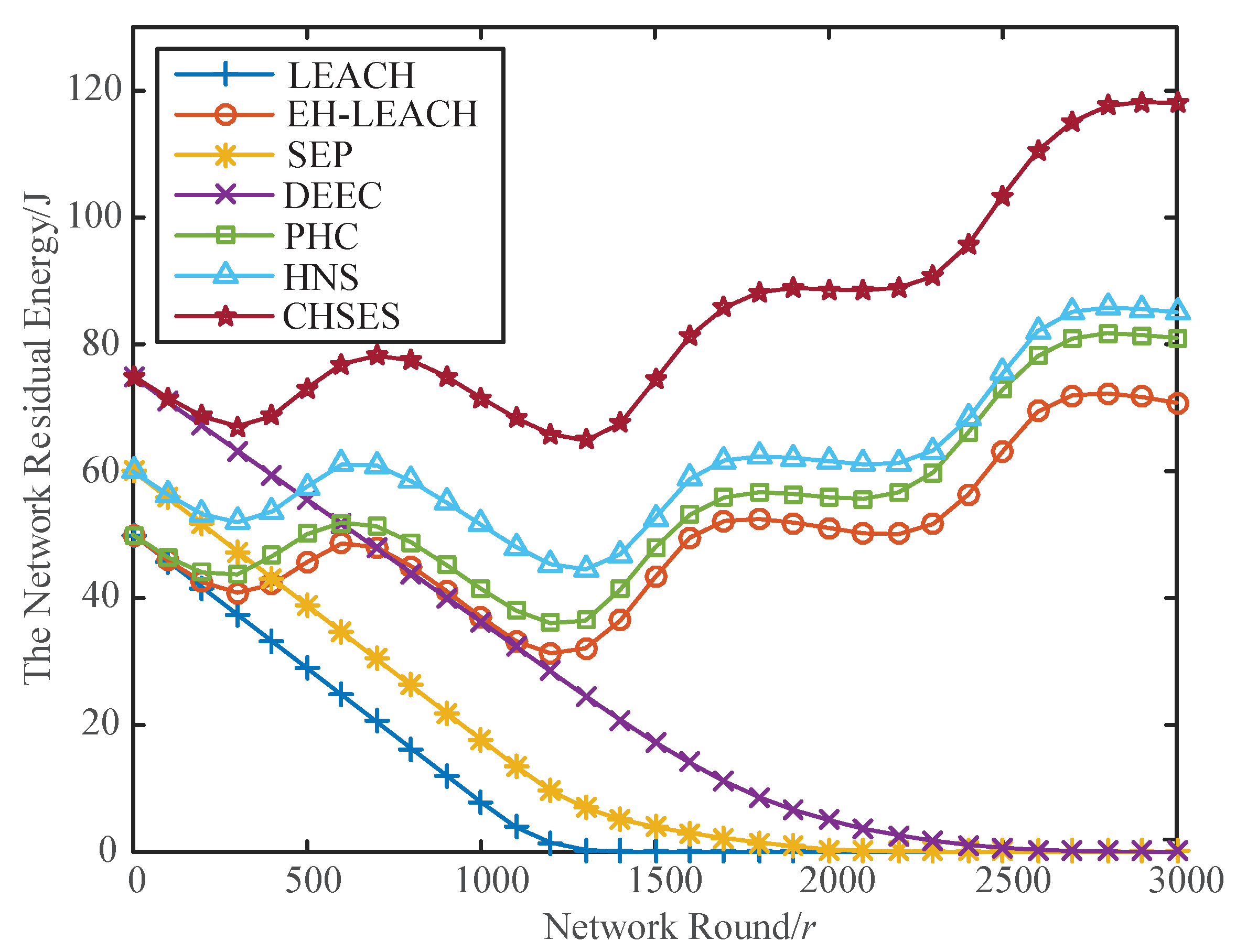
As indicated in Figure 11, the residual energy of different nodes of the algorithm decreased by varying degrees with the increase in the number of rounds. After the 300th round, the residual energies of the LEACH, SEP, and DEEC algorithms without an energy supply continued to decline. Several algorithms with energy supply received a certain amount of solar energy supply, and the residual energy of the network nodes increased. This condition indicates that an algorithm with energy replenishment can remarkably prolong the lifetime of the network.
Compared with the EH-LEACH, PHC, and HNS algorithms under the same energy supply, the CHSES algorithm is clearly better, because it uses the network initial energy classification strategy. The advantage of the CHSES algorithm in terms of the residual energy of network nodes is clear with the increase in the number of rounds. The residual energy of the network node exceeded its initial energy, specifically, after the 1500th round. This condition shows that the CHSES algorithm can optimize the cluster-head selection method and inter-cluster multi-hop mechanism, effectively balance network energy consumption, and prolong the network lifetime.
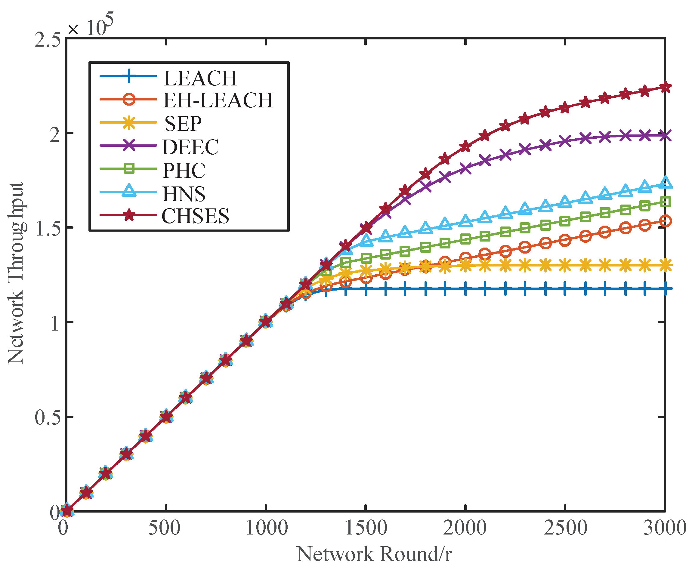
5.2.5. Comparison of Network Throughput
In WSNs, the total number of packets successfully delivered to the base station is called the throughput of the network. As illustrated in Figure 12, the throughputs of several of the algorithms were essentially the same in the first 1100th rounds and steadily increased at a relatively higher rate. This was because no dead nodes existed in the early stages of the algorithms, and the network ran relatively stably. Thus, all the packets were accurately transmitted to the base station.
After the 1500th round, significant differences were observed in the throughput of several algorithms. The LEACH and SEP algorithms without energy replenishment did not increase the network throughput after the 1500th round. The EH-LEACH, PHC, and HNS algorithms with an energy supply increased at the same rate after the 1500th round, because only a few advanced nodes and a small number of ordinary nodes were observed in the network at this time.
The network throughput of the DEEC and CHSES algorithms still increased at a high rate at the 2000th round. However, the DEEC algorithm was essentially unchanged after the 2000th round because of an insufficient energy supply. This condition indicates that the CHSES algorithm can effectively extend the network lifetime, balance the network energy consumption, and increase the network throughput.
We give the following summary on the basis of the above simulation experiments. First, the use of sensor nodes with energy collection can extend the overall network lifetime of the common non-energy-collection sensor nodes on the basis of the comparison between the original LEACH and EH-LEACH algorithms with energy supply.
The proposed CHSES algorithm can effectively prolong the network lifetime and improve the utilization of nodes by comparing the number of remaining nodes in the network. The CHSES algorithm can make the network run stably and durably by comparing the network stability period and the number of cluster heads in each round. The comparison of the residual energy of network nodes and network throughput shows that the CHSES algorithm can optimize the cluster-head selection method and the multi-hop mechanism between clusters, can effectively balance the network energy consumption, and can increase the network throughput.
6. Conclusions
In this paper, a heterogeneous sensor network clustering algorithm (CHSES) based on a solar energy supply is proposed to solve the problem of limited battery power that directly affects the performance and survival time of sensor networks. The solar energy around the node is converted into the node power supply, and the nodes are divided into advanced nodes with energy self-replenishment and energy-limited ordinary nodes. An advanced node dormancy limit is set, and cluster-head selection to balance the network energy consumption is used on the basis of the residual energy of the nodes and energy self-recharge state of advanced nodes. The mechanism is based on hierarchical multi-hop routing for data transmission. The simulation results show that the proposed algorithm effectively extends the lifetime of the network and improves the stability and energy balance of the network compared with other algorithms. Currently, energy-harvesting technology is improving. Energy-supplied nodes can be used in entire WSNs. In the future, we will design a clustering algorithm for isomorphic sensor networks with energy replenishment and optimize the energy consumption of sensor networks.
Author Contributions
C.H. mainly devised the research idea and wrote the paper. Q.L. designed and performed the experiments; J.G. and Z.T. analyzed the data; L.S. supervised the work. All the authors read and approved the final manuscript.
Funding
This work is partly funded by the National Natural Science Foundation of China under Grant Nos. 61572261, 61702284, and 61662039; the Natural Science Foundation of Jiangsu Province under Grant No. BK20150868; the Postdoctoral Fund of Jiangsu Province under Grant No. 1701165C; and the NUPTSF under Grant No. NY214013.
Conflicts of Interest
The authors declare no conflict of interest.
References
- Akyildiz, I.F.; Su, W.; Sankarasubramaniam, Y.; Cayirci, E. A survey on sensor networks. IEEE Commun. Mag. 2002, 40, 102–114. [Google Scholar] [CrossRef]
- Xiao, F.; Liu, W.; Li, Z.T.; Chen, L.; Wang, R.C. Noise-Tolerant Wireless Sensor Networks Localization Via Multi-norms Regularized Matrix Completion. IEEE Trans. Veh. Technol. 2018, 67, 2409–2419. [Google Scholar] [CrossRef]
- Akyildiz, I.F.; Vuran, M.C. Wireless Sensor Networks; John Wiley & Sons Ltd.: Hoboken, NJ, USA, 2010. [Google Scholar]
- Zordan, D.; Melodia, T.; Rossi, M. On the design of temporal compression strategies for energy harvesting sensor networks. IEEE Trans. Wirel. Commun. 2016, 15, 1336–1352. [Google Scholar] [CrossRef]
- Xiao, F.; Wang, Z.Q.; Ye, N.; Wang, R.C.; Li, X.Y. One More Tag Enables Fine-Grained RFID Localization and Tracking. IEEE/ACM Trans. Netw. 2018, 26, 161–174. [Google Scholar] [CrossRef]
- Zhu, H.; Xiao, F.; Sun, L.J.; Wang, R.C.; Yang, P.L. R-TTWD: Robust Device-free Through-The-Wall Detection of Moving Human with WiFi. IEEE J. Sel. Areas Commun. 2017, 35, 1090–1103. [Google Scholar] [CrossRef]
- Srbinovski, B.; Magno, M.; O’Flynn, B.; Pakrashi, V.; Popovici, E. Energy aware adaptive sampling algorithm for energy harvesting wireless sensor networks. In Proceedings of the 2015 IEEE Sensors Applications Symposium (SAS), Zadar, Croatia, 13–15 April 2015; pp. 1–6. [Google Scholar]
- Dehwaha, A.H.; Elmetennania, S.; Claudelb, C. UD-WCMA: An energy estimation and forecast scheme for solar powered wireless sensor networks. J. Netw. Comput. Appl. 2017, 90, 17–25. [Google Scholar] [CrossRef]
- Liu, Q.; Zhang, Q.J. Accuracy improvement of energy prediction for solar-energy-powered embedded systems. IEEE Trans. Very Large Scale Integr. Syst. 2016, 24, 2062–2074. [Google Scholar] [CrossRef]
- Visser, H.J.; Vullers, R.J.M. RF Energy harvesting and transport for wireless sensor network applications: Principles and Requirements. Proc. IEEE 2013, 101, 1410–1423. [Google Scholar] [CrossRef]
- Bozorgi, S.M.; Rostami, A.S.; Hosseinabadi, A.A.R.; Balas, V.E. A new clustering protocol for energy harvesting-wireless sensor networks. Comput. Electr. Eng. 2017, 64, 233–247. [Google Scholar] [CrossRef]
- Heinzelman, W.R.; Chandrakasan, A.; Balakrishnan, H. Energy-efficient communication protocol for wireless microsensor networks. In Proceedings of the 33rd annual Hawaii international conference on System sciences, Maui, HI, USA, 7 January 2000; pp. 3005–3014. [Google Scholar]
- Qing, L.; Zhu, Q.; Wang, M. Design of a distributed energy-efficient clustering algorithm for heterogeneous wireless sensor networks. Comput. Commun. 2006, 29, 2230–2237. [Google Scholar] [CrossRef]
- Smaragdakis, G.; Matta, I.; Bestavros, A. SEP: A stable election protocol for clustered heterogeneous wireless sensor networks. In Proceedings of the 2nd International Workshop on Sensor and Actor Network Protocols and Applications, Baltimore, MD, USA, 31 May 2004. [Google Scholar]
- Fan, X.; Yang, X.; Liu, S.; Qu, Z. Clustering routing algorithm for wireless sensor networks with power harvesting. Comput. Eng. 2008, 34, 120–122. [Google Scholar]
- Xu, X.; Lv, Q.; Wang, W.; Huangfu, X. Clustering routingalgorithm for heterogeneous wireless sensor networks with self-supplying nodes. Comput. Sci. 2017, 44, 134–139. [Google Scholar]
- Yao, Y.; Wang, G.; Ren, Z.; Yi, J. Energy balanced clustering algorithm for self-energized wireless sensor networks. Chinese J. Sens. Actuators 2013, 2013, 1420–1425. [Google Scholar]
- Roundy, S.; Wright, P.K.; Rabaey, J. A study of low level vibrations as a power source for wireless sensor nodes. Comput. Commun. 2003, 26, 1131–1144. [Google Scholar] [CrossRef]
- Zaidi, S.A.R.; Afzal, A.; Hafeez, M.; Ghogho, M.; McLernon, D.C.; Swami, A. Solar energy empowered 5G cognitive metro-cellular networks. IEEE Commun. Mag. 2015, 53, 70–77. [Google Scholar] [CrossRef] [Green Version]
- Martinez, G.; Li, S.; Zhou, C. Maximum residual energy routing in wastage-aware energy harvesting wireless sensor networks. In Proceedings of the 79th IEEE Vehicular Technology Conference (VTC Spring), Seoul, Korea, 18–21 May 2014; pp. 1–5. [Google Scholar]
- Martinez, G.; Li, S.; Zhou, C. Multi-commodity online maximum lifetime utility routing for energy-harvesting wireless sensor networks. In Proceedings of the IEEE Global Communications Conference (GLOBECOM), Austin, TX, USA, 8–12 December 2014; pp. 106–111. [Google Scholar]
- Oak Ridge National Laboratory (ORNL) RSR Web Site. Available online: http://midcdmz.nrel.gov/ornl _ rsr/ (accessed on 5 April 2018).
- Heinzelman, W.B.; Chandrakasan, A.P.; Balakrishnan, H. An application-special protocol architecture for wireless micro-sensor networks. IEEE Trans. Wirel. Commun. 2002, 1, 660–670. [Google Scholar] [CrossRef]
Figure 1.
Classic solar energy supply model (trapezoidal model).

Figure 2.
Solar energy supply model (Gaussian model).

Figure 3.
True collection of solar energy.

Figure 4.
Gaussian kernel density function under different window widths.

Figure 5.
Gaussian kernel density solar model used to simulate the true weather.

Figure 6.
Topology diagram for layered transmission of network nodes.

Figure 7.
Algorithm flow chart.

Figure 8.
Comparison of the number of remaining surviving nodes in the network.

Figure 9.
Network stability-cycle comparison.

Figure 10.
Number of cluster heads in the first 20 rounds.

Figure 11.
Comparison of the network residual energy.

Figure 12.
Comparison of network throughput.


Table 1.
Energy consumption results of setting different values of .
| 0.2 | 0.3 | 0.4 | 0.5 | 0.6 | 0.7 | |
|---|---|---|---|---|---|---|
| The round number of the first dead node | 1367 | 1173 | 1283 | 1506 | 1309 | 1337 |
Table 2.
Simulation parameter setting.
| Parameter | Parameter Meaning | Value |
|---|---|---|
| N | Number of nodes | 100 |
| Base-station coordinates | [50, 50] | |
| m | Advanced-node ratio | 0.2 |
| p | Proportion of ideal cluster heads | 0.1 |
| Initial energy of node | 0.5 J | |
| Emission circuit loss | 50 nJ/bit | |
| Energy consumption factor of free-space amplifier | 10 pJ/bit/m | |
| Energy consumption factor of | 0.0013 pJ/bit/m | |
| multi-path-attenuated power amplifier | ||
| Receiving circuit loss | 50 nJ/bit | |
| Data fusion loss | 5 nJ/bit | |
| a | Advanced node exceeds the initial | 5 nJ/bit |
| energy percentage of ordinary node | ||
| l | Packet length | 4000 bit |
| The largest round | 3000 |
Table 3.
Time comparison of death nodes.
| Algorithm | Death of First Node | Death of 10% of Nodes | Death of All Nodes |
|---|---|---|---|
| LEACH | 921 | 1053 | 1362 |
| EH-LEACH | 968 | 1063 | — |
| SEP | 1072 | 1124 | 2040 |
| DEEC | 1348 | 1487 | 2942 |
| PHC | 1085 | 1203 | — |
| HNS | 1216 | 1318 | — |
| CHSES (proposed) | 1506 | 1712 | — |
© 2018 by the authors. Licensee MDPI, Basel, Switzerland. This article is an open access article distributed under the terms and conditions of the Creative Commons Attribution (CC BY) license (http://creativecommons.org/licenses/by/4.0/).
Share and Cite
MDPI and ACS Style
Han, C.; Lin, Q.; Guo, J.; Sun, L.; Tao, Z. A Clustering Algorithm for Heterogeneous Wireless Sensor Networks Based on Solar Energy Supply. Electronics 2018, 7, 103. https://doi.org/10.3390/electronics7070103
AMA Style
Han C, Lin Q, Guo J, Sun L, Tao Z. A Clustering Algorithm for Heterogeneous Wireless Sensor Networks Based on Solar Energy Supply. Electronics. 2018; 7(7):103. https://doi.org/10.3390/electronics7070103
Chicago/Turabian StyleHan, Chong, Qing Lin, Jian Guo, Lijuan Sun, and Zhuo Tao. 2018. "A Clustering Algorithm for Heterogeneous Wireless Sensor Networks Based on Solar Energy Supply" Electronics 7, no. 7: 103. https://doi.org/10.3390/electronics7070103
Note that from the first issue of 2016, this journal uses article numbers instead of page numbers. See further details here.