A Virtual Micro-Islanding-Based Control Paradigm for Renewable Microgrids

Abstract

Improvements in control of renewable energy-based microgrids are a growing area of interest. A hierarchical control structure is popularly implemented to regulate key parameters such as power sharing between generation sources, system frequency and node voltages. A distributed control infrastructure is realized by means of a communication network that spans the micro-distribution grid. Measured and estimated values, as well as corrective signals are transmitted across this network to effect required system regulation. However, intermittent latencies and failures of component communication links may result in power imbalances between generation sources, deviations in node voltages and system frequency. This paper proposes a hierarchical control structure to regulate the operation of an islanded AC microgrid experiencing communication link failures. The proposed strategy aims to virtually sub-divide the microgrid into controllable “islands”. Thereafter, active power sharing, frequency and voltage restoration is achieved by competing converter systems through multi-agent consensus. The effectiveness of the proposed methodology has been verified through stability analyses using system wide mathematical small signal models and case study simulations in MATLAB, Simpower systems.

1. Introduction

Recent advances in renewable energy technologies have led to a greater penetration of distributed renewable energy resources (DERs) in power distribution networks. However, due to the stochastic nature of renewable energy resources, Distributed Generation Units (DGUs) suffer from voltage deviations, frequency and power flow variations. Micro-grids (MGs) present a viable solution to the renewable energy integration problem. A micro grid is usually composed of a smaller power distribution network, energy sources, energy storages, Electric Vehicles (EV), DGUs, supervisory control and data acquisition devices. The MG behaves as a smaller isolated power system that can operate either as an energized island or in synchrony with the legacy power network. Local control measures are applied within the micro-grid to address voltage, frequency and power flow deviations [1,2,3,4].

Power conversion stages of multiple DGUs operate in parallel through the MG distribution network. Proportional sharing of power between various DGUs is required to ensure stable system operation and fair power contribution by each generation source in a microgrid. Droop control methods are employed as a simple decentralized strategy for sharing total load power among DGUs. Active and reactive power fractions proportional to frequency and amplitude respectively, are subtracted from converter output. This method is commonly referred to as P-f and Q-E droop method and has been previously used in the control of un-interruptible power supply systems (UPS) [5,6,7,8,9,10]. Although, the droop methods provide a degree of reliability, there are certain drawbacks associated therewith. P-f/Q-E droop control works on the principle of reducing frequency and voltage by fractions to achieve power sharing. To keep the system voltage and frequency within a permissible range, a secondary control layer must be implemented to periodically correct these deviations. This can be realized through a centralized hierarchical control; composed of three or more control layers; or a decentralized control strategy where local nodes share information that modifies voltage and frequency references for inner control loops [10,11,12,13,14].

Most centralized control algorithms require a two-way transmission of information between DGUs throughout the system and Microgrid central controllers (MGCC). Such a control structure is often complicated and expensive to implement, in addition to being susceptible to single point of failure (SPOF). Therefore, a decentralized control approach employing consensus algorithms, has emerged as an alternate to centralized control methods [2,15,16,17]. Consensus-based methods model the frequency and voltage restoration goals as a multi-agent consensus problem; where, each power converter behaves as an agent regulating its voltage and frequency in combination with other agents (nodes), collectively arriving at consensus values for V and f. A virtual leader node may provide desired nominal values for controlled parameters to the micro grid controls [2,18,19].

Some researches propose a secondary voltage restoration method based on distributed cooperative control of multi-agent systems [12], wherein individual inverter units are considered as systems having non-linear internal dynamics. Input-Output feedback linearization is used to convert the secondary voltage restoration problem in such units into a second order linear tracker synchronization problem. The authors in [20] explore active power sharing in islanded AC microgrid with secondary control of frequency and voltage restoration. The inverters have been modeled as cooperative multiagent systems such that their frequency and voltage restoration be a synchronization problem. In [21], the authors present a consensus-based distributed secondary restoration control for both frequency and voltage in droop-controlled AC microgrids.

The authors in [22], present a distributed secondary control method for an inverter-based microgrid with uncertain communication links. The method discussed addresses active power flow control and restoration of frequency and voltage to nominal values. In [23], a distributed control strategy for reactive power sharing and voltage restoration in AC microgrids is presented. The strategy discussed uses small signal model of the system and sensitivity analysis to evaluate the relationship between voltage magnitude and reactive power sharing. In [24], authors have proposed a consensus-based distributed voltage control algorithm for islanded inverter-based microgrids with arbitrary meshed electrical topologies. This algorithm is based on weighted average consensus protocol that replaces traditional V-Q droop method.

The authors in [25] present a dynamic consensus algorithm (DCA) for coordinated control with an autonomous current sharing control strategy to balance discharge rate of energy storage systems (ESS) in an islanded AC microgrid. The DCA is used to share information between DG converter units to regulate output power according to ESS capacities and battery state of charge. In [26] authors propose a cooperative distributed control method for AC microgrids that discusses an alternate for the centralized secondary control and the primary-level droop mechanism of each inverter. Voltage, reactive power, and active power regulators are employed to achieve regulation of these parameters.

The work presented in [12,20,21,23,24] assumes a fault-free communication network with no broken or disrupted communication links. The communication digraph used is, therefore, time in-varying. However, the studies presented in [22,25,26] discuss scenarios with faulty communication links. The authors in [25] have represented faulty communications through a dynamically varying digraph.

This work proposes a hybrid, multi-agent consensus-based control strategy to realize power sharing, voltage and frequency regulation for an islanded AC microgrid. The method developed here addresses faults created by faulty communication links through virtually isolating portions of the network suffering from communication faults and intermittencies. Thereafter, the control parameters are tuned to treat these isolated portions as smaller “virtual micro-grids” within the larger micro-gird. The salient contributions of this work are:

• Identification of failed communication links.
• Virtual segmentation of the MG network into smaller controllable islands.
• Variation in droop and consensus control parameters to achieve power sharing, voltage and frequency restoration during communication faults.
• Using small signal analysis to study MG system stability under the proposed control scheme.

The rest of the paper is divided as follows: Section 2 gives the microgrid network layout, derives the admittance matrix and fundamental power flow equations. Section 3 describes the hierarchical control paradigm proposed. Section 4 gives details of the communication network layer and basic graph theoretic definitions. Section 5 expounds the virtual sub islanding method used in this work. Section 6 gives small signal system derivation. Section 7 presents the results of stability analysis using eigen evolutions. Section 8 gives case study simulations and results. Section 9 concludes the paper.

2. Network Layout

This section describes the network layout and derives the admittance matrix and fundamental power flow equations. Figure 1 represents a simplified radial type three phase three wire system used in this study and the proposed four level control strategy. Buses 1 through 6 are fed through power electronic converters interfaced with the network using LC filters. The buses 2 through 6 are directly loaded with adjustable power loads whereas bus-1 is not directly loaded. This network can be operated in islanded mode.

Table 1. System parameters for microgrid control.

Parameters	Values	Parameters	Values
Lf	1.35 mH	mp	4.5 × 10 −6
Rf	0.1 Ω	nq	1× 10 −6
Cf	25 µF	Kpf	0.4
Lc	1.35 mH	Kif	0.5
Rc	0.05 Ω	KpV	0.5
Rline	0.1 Ω	KiV	0.3
Lline	0.5 mH	F	1
fnom	60 Hz	ωc	60 Hz
Vnom	415 VL-L

outlines rated system parameters and

Table 2. System loads.

Bus. No.	Directly Connected Bus Load
	P (p.u.)	Q (p.u.)
1.	0	0
2.	0.3	0.3
3.	0.25	0.25
4.	0.25	0.25
5.	0.25	0.25
6.	0.25	0.25
7.	0	0

gives bus loads. All distributed renewable generators are represented by equivalent DC sources. Later sections describe the multi-level control methodology in detail.

Equation (1) Gives the combined bus admittance matrix of micro network. Equation (2) gives the steady state model of the system.

$$Y_{busMG}=\left[\begin{array}{ccccccc}(Y_{s1}+Y_{17}+Y_{12})& -Y_{12}& 0& 0& 0& 0& -Y_{17}\\ -Y_{21}& (Y_{s2}+Y_{23}+Y_{12})& -Y_{23}& 0& 0& 0& 0\\ 0& -Y_{32}& (Y_{s3}+Y_{32}+Y_{34})& -Y_{34}& 0& 0& 0\\ 0& 0& -Y_{43}& (Y_{s4}+Y_{43}+Y_{45})& -Y_{45}& 0& 0\\ 0& 0& 0& -Y_{54}& (Y_{s5}+Y_{54}+Y_{56})& -Y_{56}& 0\\ 0& 0& 0& 0& -Y_{65}& (Y_{s6}+Y_{65})& 0\\ -Y_{71}& 0& 0& 0& 0& 0& (Y_{71}+Y_{s7})\end{array}\right]$$

(1)

$$\left[Y_{busMG}\right]•{\left[\begin{array}{ccccccc}{V}_1& V_2& V_3& V_4& V_5& V_6& V_7\end{array}\right]}^T={\left[\begin{array}{ccccccc}{I}_{s1}& I_{s2}& I_{s3}& I_{s4}& I_{s5}& I_{s6}& I_{s7}\end{array}\right]}^T$$

(2)

where Y_si represents the inverter (source) LCL coupling admittance; Y_ij represents the line admittance between i^th and j^th busses (nodes); I_si represents the current injected into the i^th bus. The active and reactive powers injected at each node can be given by (3) and (4).

$$P_i={\displaystyle \sum }_{n=1}^N\left|Y_{in}{V}_i{V}_n\right|·\cos \left({\theta }_{in}+{\delta }_n-{\delta }_i\right)$$

(3)

$$Q_i=-{\displaystyle \sum }_{n=1}^N\left|Y_{in}{V}_i{V}_n\right|·\sin \left({\theta }_{in}+{\delta }_n-{\delta }_i\right)$$

(4)

where, Y_in is the admittance connected between i^thand n^th bus; V_iis the voltage magnitude at i^th inverter terminal and V_n is voltage magnitude at the n^th bus; ${\theta }_{in}$ is the admittance angle between bus ith and nth bus,${\delta }_n$ is voltage angle at n^th bus whereas ${\delta }_i$ is the voltage angle at i^th bus.

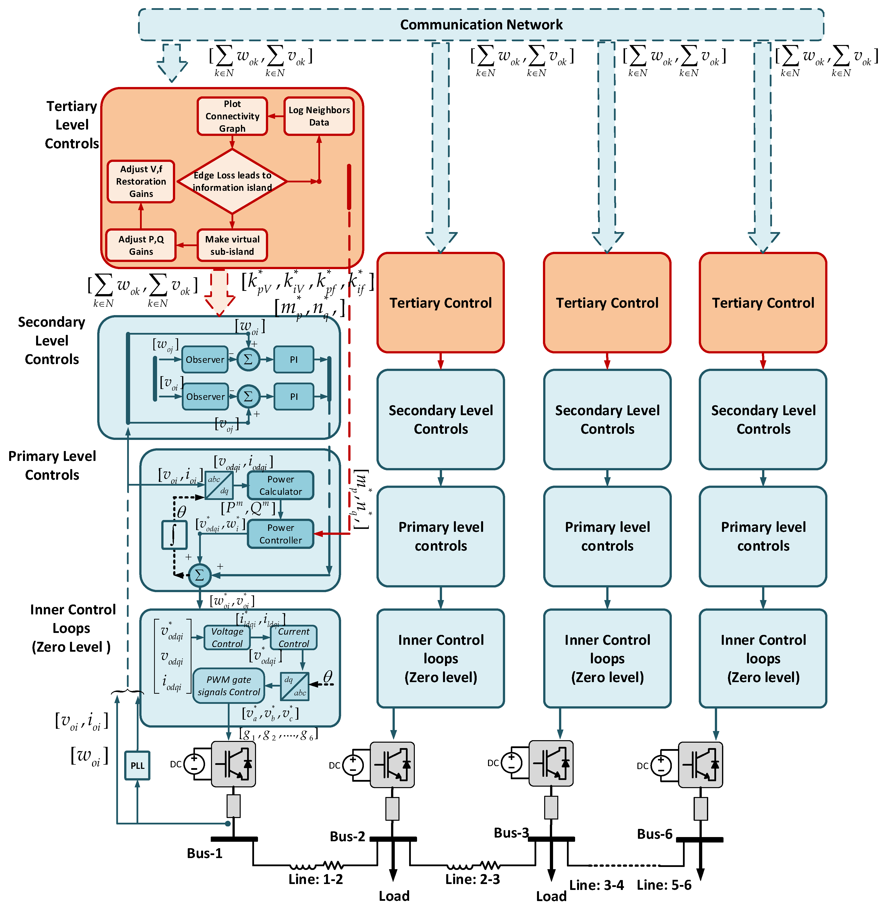
3. Hierarchical Control Paradigm

This section elaborates on the hierarchical control structure implemented to regulate the microgrid network. the distributed control paradigm is divided into four layers, as shown in Figure 1. The inner, or zero level controls, consist of current and voltage control loops that regulate basic local dynamics. The primary level controls address power balancing between converter nodes. The secondary level controls serve to correct voltage and frequency deviations created by primary control action. The zero level, primary and secondary controls are further elaborated in Figure 2a–d. This work proposes a tertiary level control, aimed at detecting communication link failures and mitigating their effect by creating smaller virtual sub-islands within the microgrid and regulating their performance by modifying secondary and primary controller parameters. The tertiary controls absorb and process frequency and voltage measurements $({\displaystyle \sum }_{k\in N}{\omega }_{ok},{\displaystyle \sum }_{k\in N}{\upsilon }_{ok})$, from node neighborhood. Once the status of connectivity of the network has been determined as described in Section 5, updated references for voltage and frequency PI gains in secondary control $K_{pV}{}^{*},K_{iV}{}^{*},K_{pf}{}^{*},K_{if}{}^{*}$, and droop gains $m_p{}^{*},n_p{}^{*}$ are passed down to secondary and primary levels.

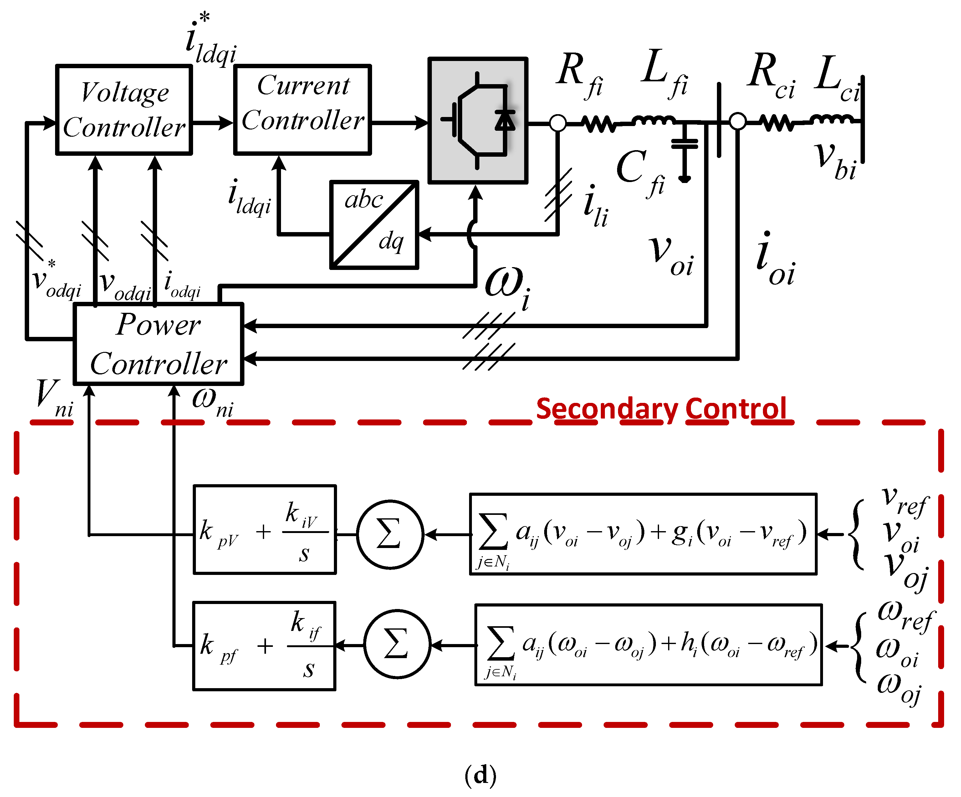
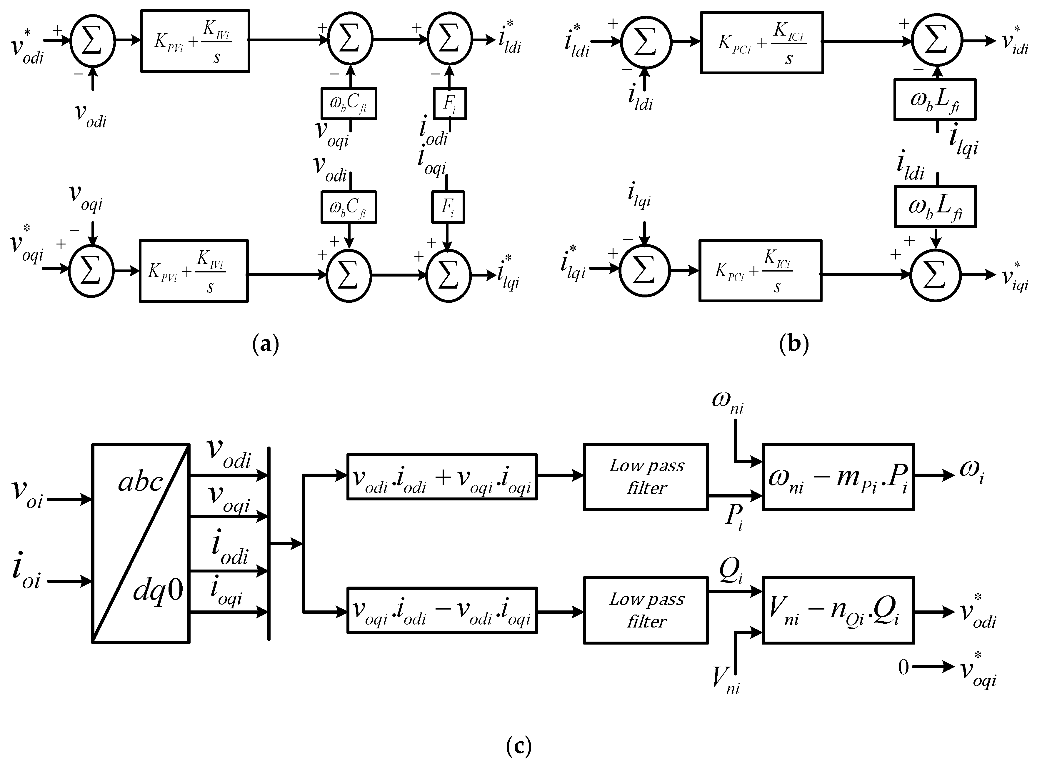
3.1. Zero Level Control loops: Voltage and Current Regulation

Voltage and current control loops in d-q-0 frame form the zero level control loops for each of the power converters as shown in Figure 2a,b. dynamical equations for voltage control loop are given as (5) and (6).

$$\begin{array}{c}\frac{d{\varphi }_{di}}{dt}={\varphi }_{di}^{\prime }=u_{odi}^{*}-u_{odi}\\ \frac{d{\varphi }_{qi}}{dt}={\varphi }_{qi}^{\prime }=u_{oqi}^{*}-u_{oqi}\end{array}\}$$

(5)

$$\begin{array}{c}{i}_{ldi}^{*}=F_i·i_{odi}-{\omega }_b·C_{fi}·u_{oqi}+K_{PVi}\left(u_{odi}^{*}-u_{odi}\right)+K_{IVi}{\varphi }_{di}\\ i_{lqi}^{*}=F_i·i_{oqi}-{\omega }_b·C_{fi}·u_{odi}+K_{PVi}\left(u_{oqi}^{*}-u_{oqi}\right)+K_{IVi}{\varphi }_{qi}\end{array}\}$$

(6)

where, K_PVi and K_IVi represent the proportional and integral gains of the voltage controller. ${\varphi }_{di}$ and ${\varphi }_{qi}$ are auxiliary state variables for the PI controllers. F_i is the feed-forward gain. v_oqi, v_odi, i_odi and i_oqi are system measurements as seen in Figure 2d.

Similarly, (7) and (8) represent the dynamical model for current control loop at each node as shown in Figure 2b.

$$\begin{array}{c}\frac{d{\varsigma }_{di}}{dt}={\varsigma }_{di}^{\prime }=i_{ldi}^{*}-i_{ldi}\\ \frac{d{\varsigma }_{qi}}{dt}={\varsigma }_{qi}^{\prime }=i_{lqi}^{*}-i_{lqi}\end{array}\}$$

(7)

$$\begin{array}{c}{u}_{idi}^{*}=-{\omega }_b·L_{fi}·i_{lqi}+K_{PCi}\left(i_{ldi}^{*}-i_{ldi}\right)+K_{ICi}{\varsigma }_{di}\\ u_{iqi}^{*}={\omega }_b·L_{fi}·i_{ldi}+K_{PCi}\left(i_{lqi}^{*}-i_{lqi}\right)+K_{ICi}{\varsigma }_{qi}\end{array}\}$$

(8)

where, K_PCi and K_ICi represent the proportional and integral gains of the voltage controller. ${\varsigma }_{di}$ and ${\varsigma }_{qi}$ are auxiliary state variables for the PI controllers used. i_lqi and i_ldi are system measurements as seen in Figure 2d.

3.2. Primary Controls: Power Balancing between Distributed Sources

Power sharing control is based on so called “droop” principle [27], i.e., frequency and voltage are proportionally reduced to achieve active and reactive power sharing respectively as shown in Figure 2c. Equations (9) and (10) represent the droop controller.

$${\omega }_i^{*}={\omega }_i-m_{Pi}·\left(P_i\right)$$

(9)

$$\begin{array}{c}{V}_{di}^{*}=V_{di}-n_{Qi}·\left(Q_i\right)\\ V_{qi}^{*}=0\\ V_o=\sqrt{V_{di}^{*}{}^2+V_{qi}^{*}{}^2}\end{array}\}$$

(10)

where, ${\omega }_i$ and $V_0$ are the nominal references of frequency and voltage for the ith inverter. $P_i$ and $Q_i$ correspond to active and reactive power being injected by the i^th power inverter at output terminals. $m_{Pi}$ and $n_{Qi}$ are droop gains that can be calculated as (11).

$$\{\begin{array}{c}{m}_{Pi}=\frac{\Delta \omega }{Pmax}\\ n_{Qi}=\frac{\Delta V}{Qmax}\end{array}$$

(11)

where, $\Delta \omega$ and $\Delta V$ are the maximum change permissible for converter frequency and voltage respectively. Pmax and Qmax are the maximum active and reactive power the converter can deliver [12]. Primary control calculates power using two-axis theory. For accurate measurement of the fundamental power component low pass filters are used having cut off frequency of ${\omega }_{ci}$. The reference frames of all inverters may be converted a common reference frame. The angle difference between i^th inverter and common frequency reference frame can be shown as (12)

$$\delta =\int \left(\omega -{\omega }_{com}\right)·dt$$

(12)

where, ${\omega }_{com}$ is the MG common system frequency.

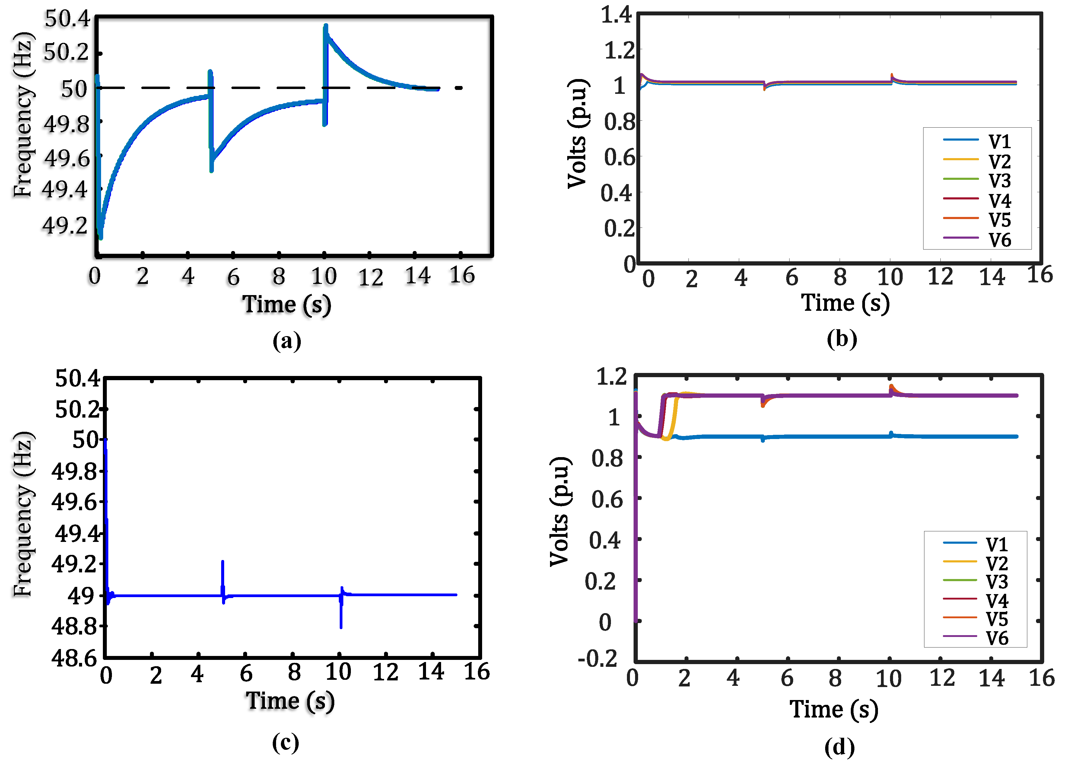
3.3. Secondary Controls: Voltage Magnitude and Frequency Restoration

Voltage magnitude and frequency restoration is achieved through multiagent consensus-based secondary control implemented at each node [28]. Figure 2d shows the distributed frequency and voltage restoration control schemes. Frequency regulation method is given by (13).

$$\begin{array}{c}\delta {\omega }_i\left(t\right)=k_{pf}{e}_{\omega i}\left(t\right)+k_{if}\int e_{\omega i}\left(t\right)·dt\\ e_{\omega i}\left(t\right)={\displaystyle \sum }_{j\in N_i}\begin{array}{c}{a}_{ij}\left({\omega }_{oi}\left(t\right)-{\omega }_{oj}\left(t\right)\right)\\ +h_i\left({\omega }_{oi}\left(t\right)-{\omega }_{ref}\left(t\right)\right)\end{array}\end{array}\}$$

(13)

where, ${\omega }_{ref}$ is the nominal reference frequency, ${\omega }_{oj}$ is the measured system frequency sensed at all nodes in the neighborhood of the i^th node being considered. k_pf and k_if are proportional and integral gains as shown in Figure 2d. $\delta {\omega }_i$ is the frequency correction applied to frequency reference of the i^th inverter node. $h_i$ is pinning gain whose value is zero for primary node.

The voltage regulation method is described in (14):

$$\begin{array}{c}\delta V_i=k_{pv}{e}_{vi}+k_{iv}\int e_{vi}dt\\ e_{vi}\left(t\right)={\displaystyle \sum }_{j\in N_i}\begin{array}{c}{a}_{ij}\left(v_{oi}\left(t\right)-v_{oj}\left(t\right)\right)\\ +g_i\left(v_{oi}\left(t\right)-v_{ref}\left(t\right)\right)\end{array}\end{array}\}$$

(14)

where, $v_{nom}$ is the nominal reference voltage for the system in p.u., $v_{oj}$ is the system voltage sensed at all converter nodes in the communication neighborhood of the node ibeing considered. k_pv and k_iv are proportional and integral gains as shown in Figure 2d. $\delta V_i$ is the voltage correction applied to voltage reference of the i^th inverter node.$g_i$ is pinning gain whose value is zero for primary node.

4. Communication Network

The communication network used to exchange information between DGs can be modelled as a digraph. A digraph is usually expressed as $G_{com}=\left(V_g{E}_g{A}_g\right)$ which is composed of a non-empty, finite set of M nodes given by $V_g=\left\{v_1{v}_2{v}_3\dots v_M\right\}$. The arcs that connect these nodes are given by $E_g\subset V_g\times V_g$. The associated adjacency matrix is given by $A_g=\left[a_{ij}\right]\in R^{N\times N}$. In a microgrid, the DGs can be thought of as the nodes of a communication digraph whereas the arcs represent communication links [28].

In this work, it is assumed that the communication network is initially stable and time invariant as represented in Figure 3a. However, communication links are made to break in analysis given in later sections of the paper. Channel noise has been neglected for simplifying calculations. Therefore, the representative digraph is also initially time invariant, i.e., $A_g$ is a constant. An arc from node j to node i is denoted by $\left(v_j,v_i\right)$, where node j receives information from node i. a_ij is the weight of the arc connecting v_i to v_j. $a_{ij}>0$, if $\left(v_j,v_i\right)\in E_g$, otherwise $a_{ij}=0$. Node i is called a neighbor of node j, if the arc$\left(v_j,v_i\right)\in E_g$. Set of nodes neighboring the ith DGU $v_i$are given by $N_i=\{v_j\in V_g:\left(v_i,v_j\right)\in E_g$}. The Laplacian Matrix $L_g={\left(l_{ij}\right)}_{N\times N}$ is defined as $l_{ij}=-a_{ij},i\ne j$ and $l_{ii}={{\displaystyle \sum }}_{j-1}^N{a}_{ij}\mathrm{for}i=1,\dots ,N.$ Such that $L_{1N}=0$ with $1_N={\left(1,\dots ,1\right)}^T\in R^N$. The in-degree matrix can be defined as $D_G^{in}=diag\left\{d_i^{in}\right\}$, where, $d_i^{in}={\displaystyle \sum }_{j\in N_i}(a_{ji})$and out-degree matrix as $D_G^{out}=diag\left\{d_i^{out}\right\}$, where $d_i^{out}={{\displaystyle \sum }}_{i\in N_i}\left(a_{ji}\right)$. The diagonal pinning gain matrix is given by$G=diag\left\{g_i\right\}$. The system adjacency, degree and Laplacian matrix are given in Appendix C.

The multiagent consensus algorithms implemented across the MG system converge over time according to [29]. The global system dynamics can therefore be given as (15) and (16).

$$\dot{x}=-\left({\mathit{D}}_{\mathit{g}}+{\mathit{G}}_{\mathit{g}}\right)x+{\mathit{A}}_{\mathit{g}}x=-\left({\mathit{D}}_{\mathit{g}}+{\mathit{G}}_{\mathit{g}}-{\mathit{A}}_{\mathit{g}}\right)x+G{x}_0$$

(15)

where,

$$\dot{x}=-\left({\mathit{L}}_{\mathit{g}}+{\mathit{G}}_{\mathit{g}}\right)x+G{\underset{\_}{x}}_0$$

(16)

and,

$${\underset{\_}{x}}_0=1x_0={\left[x_o\dots x_0\right]}^T$$

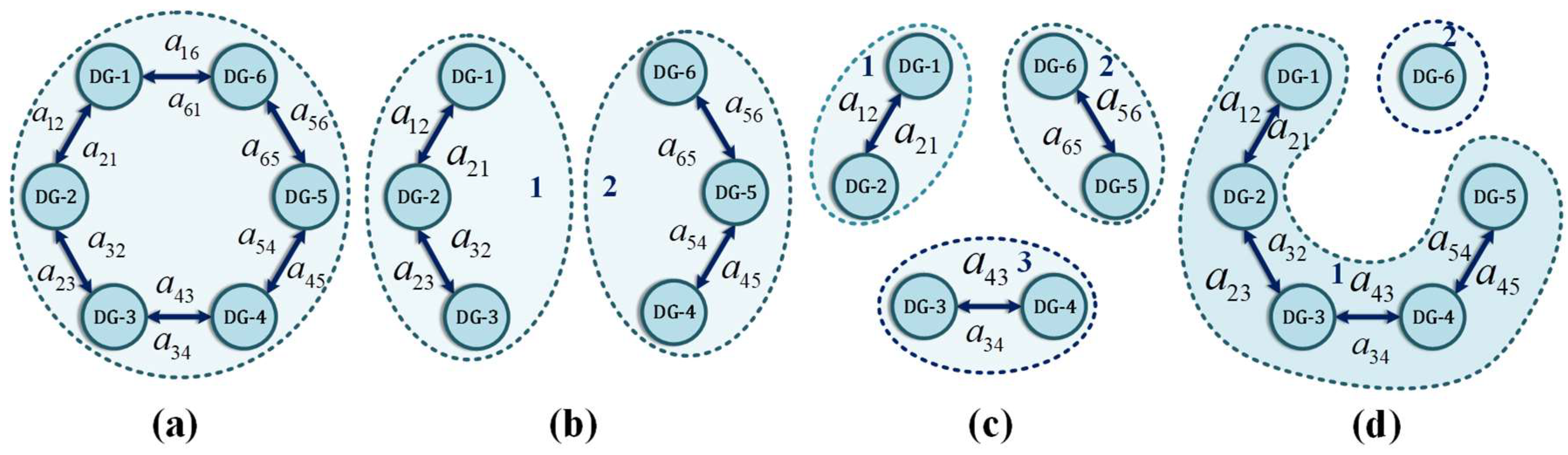
5. Virtual Sub-Islanding: Tertiary Controls

In this section, tertiary controls are presented here that monitor network connectivity. When link breakage is detected the microgrid network is virtually partitioned into sub-networks determined by connectivity of healthy communication links as described in Figure 3b,d. The supervisory consensus gains in the secondary control loop and primary control droop gains are subsequently updated to regulate power sharing and frequency voltage regulation. The following subsections further elaborate these functions.

5.1. Cut Set Enumeration

Cut set enumeration is used to analyze virtual segmentation of the microgrid network into major and minor sub-islands. A cut set of a connected graph or nodes may be defined as set of edges whose removal can disconnect the graph or nodes. Therefore, a cut set divides a graph into exact components and can subsequently be used to denote a partition of the vertices [30,31]. If $V_g$ denotes the vertex of graph $G$, and if $P_g$ is the subset of vertices in one component of graph $G$ induced by a cut set, then the cut set can be represented by, $\left(P_g,{\overline{P}}_g\right)$, where ${\overline{P}}_g=V_g-P_g$. The cut set space for a graph with $n$ vertices has dimensions of $\left(n-1\right)$.

5.2. Depth First Search Algorithm

The Depth First Search (DFS) algorithm is used to analyze graph connectivity. A graph $G_{com}$ consists of vertices $V_g$ and edges $E_g$. Initially all vertices are considered as un-visited. The DFS algorithm starts from any vertex of the graph and follows an edge until it reaches next vertex $V_g$. While choosing an edge to traverse, an edge emanating from an un-visited vertex is always chosen. A set of old vertices $V_g$ with possible unvisited edges are stored in memory [32,33]. The updated Laplacian matrix then can be obtained as $L_g=D_g^{in}-A_g$ [32,34,35].

The following Lemmas elaborate the formation of cut-sets:

Lemma 1.

A vertex cut set for graph $G_{com}=\left(V_g,E_g\right)$ is a sub set of $V_g$, whose removal will result into a disconnected graph. The vertex connectivity of graph $G_{com}$, represented by $k_0\left(G_{com}\right)$, is the minimum number of vertices in any of its vertex cut set. Assuming N nodes form a graph, if two sub sets become disconnected from each other, one of these sets of agents/ nodes are considered lost [33]. Since there are two such sets created, the smaller of the two will be considered as lost. We can define a ratio as:

$$\varnothing \left(S\right)=\frac{\epsilon \left(S,S^c\right)}{\min \left\{card\left(S\right),card\left(S^c\right)\right\}}$$

(17)

where, $\epsilon \left(S,S^c\right)$ is the number of disconnected nodes, $card\left(S\right)$ and $card\left(S^c\right)$ are the number of nodes in sub sets.

Cheeger’s Inequality [33] states that:

$$\varnothing \left(S\right)\ge {\lambda }_2\left(G_{com}\right)\ge \frac{\varnothing {\left(G_{com}\right)}^2}{2d_{max}\left(G_{com}\right)}$$

(18)

Lemma 2.

Let graph $G_{com}=\left[V_g,E_g\right]$, for each vertex $v\in V_g$ (node) creates a lookup table that contains all vertices $w$, such that $\left(v,w\right)\in E_g$. This lookup table is called adjacency matrix for vertex $V_g$. A set of lookup tables at each node (vertices) in graph G_com is called adjacent structure for graph G_com. A graph may have many adjacency structures because every edge around a vertex gives an adjacency structure and every structure leads to a unique arrangement of edges at each vertex.

The Depth First Search method (DFS) described in Appendix B [32] functions efficiently using the adjacency structure producing set of edges $\left(E_g\right)$. DFS algorithm is here labeled depth first index, $DFI\left(v\right)$ for every vertex $V_g$. Initially the value is equal to zero, whereas on the last iteration, the $DFI\left(v\right)$ is the order of last visited vertex $V_g$. The complexity of the algorithm is $O\left(\max \left(n,\left|E_g\right|\right)\right)$. For every $v\in V$, $DFI\left(v\right)$ Is called only once after it will be $DFI\left(v\right)=0$. DFS algorithm total time proportional to $\left|E_g\right|$.

The proposed method uses each node to maintain a communication link table of all known nodes throughout the micro network. These tables are updated following an exchange of information between neighboring nodes. When one or more communication links fail partially or completely, as shown in Figure 3b–d, the proposed algorithm virtually segments the network into smaller “virtual” sub micro grids. The control parameters for these scenarios are determined by arriving at good tradeoffs between system stability and better performance for each case. Eigen evolutions are used to arrive at these optimized values that are then stored in lookup tables, as shown in

Table 3. Controller parameters for analyzed cases.

Cases	Description	Secondary Consensus Gain			Primary Droop Gain
1.	Full ring network	Voltage	KpV	0.5	mp	1.0 × 10−10
			KiV	0.1
		Frequency	Kpf	0.4	nq	1.0 × 10−7
			Kif	0.1
2.	Two symmetrical islands formed	Voltage	KpV	0.7	mp	1.0 × 10−5
			KiV	0.2
		Frequency	Kpf	0.8	nq	1.0 × 10−3
			Kif	0.2
3.	Three symmetrical islands formed	Voltage	KpV	1.2	mp	2.5 × 10−3
			KiV	0.3
		Frequency	Kpf	1.5	nq	1.0 × 10−3
			Kif	0.2
4.	Two asymmetrical islands formed	Voltage	KpV	3.0	mp	2.0 × 10−4
			KiV	0.5
		Frequency	Kpf	2.2	nq	1.0 × 10−4
			Kif	0.5

, that updated droop gains (m_p*, n_q*) and consensus gains (K_pV *, K_iV *, K_pf *, K_if *) accordingly.

6. Small Signal Analysis of Microgrid System

To evaluate the performance of a proposed control method, small signal analysis of the MG system is undertaken [29,36]. Large signal dynamical equations are perturbed to obtain small signal model of the entire MG system. This section elaborates the small signal model components used in development and analysis of the control scheme.

6.1. Zero Level Converter Control Model

Small signal model for voltage control are given as in Equations (19)–(22), obtained by perturbing respective dynamical equations around quiescent point at which stability analysis is required [37,38].

$$\Delta {\varphi }_{di}={\varphi }_{di}^{\prime }=\Delta v_{odi}^{*}-\Delta v_{odi}$$

(19)

$$\Delta {\varphi }_{qi}={\varphi }_{qi}^{\prime }=\Delta v_{oqi}^{*}-\Delta v_{oqi}$$

(20)

$$\Delta i_{ldi}^{*}=F_i·\Delta i_{odi}-{\omega }_b·C_{fi}·\Delta v_{oqi}+K_{PVi}\left(\Delta v_{odi}^{*}-\Delta v_{odi}\right)+K_{IVi}{\varphi }_{di}$$

(21)

$$\Delta i_{lqi}^{*}=F_i·\Delta i_{oqi}-{\omega }_b·C_{fi}·\Delta v_{odi}+K_{PVi}\left(\Delta v_{oqi}^{*}-\Delta v_{oqi}\right)+K_{IVi}{\varphi }_{qi}$$

(22)

where, K_PVi and K_IVi represent the proportional and integral gains of the voltage controller. $\Delta {\varphi }_{di}$ and $\Delta {\varphi }_{qi}$ are perturbations in auxiliary state variables for the PI controllers. F_i is the feed-forward gain. v_oqi, v_odi, i_odi and i_oqi are system measurements as described before.

Similarly, Equations (23)–(26) represent the small signal model for current control loop at each node as shown in Figure 2b.

$$\Delta {\varsigma }_{di}={\varsigma }_{di}^{\prime }=\Delta i_{ldi}^{*}-\Delta i_{ldi}$$

(23)

$$\Delta {\varsigma }_{qi}={\varsigma }_{qi}^{\prime }=\Delta i_{lqi}^{*}-\Delta i_{lqi}$$

(24)

$$\Delta v_{idi}^{*}=-{\omega }_b·L_{fi}·\Delta i_{lqi}+K_{PCi}\left(\Delta i_{ldi}^{*}-\Delta i_{ldi}\right)+K_{ICi}·\Delta {\varsigma }_{di}$$

(25)

$$\Delta v_{iqi}^{*}={\omega }_b·L_{fi}·+K_{PCi}\left(\Delta i_{lqi}^{*}-\Delta i_{lqi}\right)+K_{ICi}·\Delta {\varsigma }_{qi}$$

(26)

where, K_PCi and K_ICi represent the proportional and integral gains of the voltage controller. $\Delta {\varsigma }_{di}$ and $\Delta {\varsigma }_{qi}$ are perturbations in auxiliary state variables for the PI controllers used. i_lqi and i_ldi are system measurements as described before in Section 3.

6.2. Primary Power Sharing Control Model

The linearized small signal model for power controller can be written as Equations (27) and (28). The power controller provides operating frequency for the DGU (ω_i) and reference voltage (v_odi* and v_oqi*) for voltage control loop [12].

$$\dot{\Delta P}=-{\omega }_{ci}\Delta P_i+{\omega }_{ci}\left(I_{od}\Delta v_{od}+I_{oq}\Delta v_{oq}+V_{od}\Delta i_{od}+V_{oq}\Delta i_{oq}\right)$$

(27)

$$\dot{\Delta Q}=-{\omega }_{ci}\Delta Q_i+{\omega }_{ci}\left(I_{oq}\Delta v_{od}-I_{od}\Delta v_{oq}-V_{oq}\Delta i_{od}+V_{od}\Delta i_{oq}\right)$$

(28)

where $I_{od}$,$I_{oq}$, $V_{od}$ and $V_{oq}$ represent steady state values of $i_{od}$,$i_{oq}$,$v_{od}$, $v_{oq}$ as in Figure 2c,d. ${\omega }_{ci}$is the cut-off frequency for low pass filters employed in the power calculator.

Small signal model of frequency and voltage control are given by (29) and (30):

$$\begin{array}{c}\Delta \omega =-m_p·\Delta P\\ \Delta v_{od}^{*}=-n_q·\Delta Q\\ \Delta v_{oq}^{*}=0\end{array}\}$$

(29)

$$\Delta \dot{\delta }=\Delta \omega -\Delta {\omega }_{com}=-m_p·\Delta P-\Delta {\omega }_{com}$$

(30)

6.3. Grid-Side Filter Model

The small signal model for the LC output filter can be given by Equations (31)–(36):

$$\dot{\Delta i_{ldi}}=-\frac{R_{fi}}{L_{fi}}·\Delta i_{ldi}+{\omega }_i·\Delta i_{lqi}+\frac{1}{Lfi}·\Delta v_{idi}-\frac{1}{Lfi}·\Delta v_{odi}+I_{lq}·\Delta \omega$$

(31)

$$\dot{\Delta i_{lqi}}=-\frac{R_{fi}}{L_{fi}}·\Delta i_{lqi}-{\omega }_i·\Delta i_{ldi}+\frac{1}{Lfi}·\Delta v_{iqi}-\frac{1}{Lfi}·\Delta v_{oqi}+·\Delta \omega$$

(32)

$$\dot{\Delta v_{odi}}={\omega }_i·\Delta v_{oqi}+\frac{1}{Cfi}·\Delta i_{ldi}-\frac{1}{Cfi}·\Delta i_{odi}+V_{oq}·\Delta \omega$$

(33)

$$\dot{\Delta v_{oqi}}={\omega }_i·\Delta v_{odi}+\frac{1}{Cfi}·\Delta i_{lqi}-\frac{1}{Cfi}·\Delta i_{oqi}-V_{od}·\Delta \omega$$

(34)

$$\dot{\Delta i_{odi}}=-\frac{R_{ci}}{L_{ci}}·\Delta i_{odi}+{\omega }_i·\Delta i_{oqi}+\frac{1}{L_{ci}}·\Delta v_{odi}-\frac{1}{L_{ci}}·\Delta v_{bdi}+I_{oq}·\Delta \omega$$

(35)

$$\dot{\Delta i_{oqi}}=-\frac{R_{ci}}{L_{ci}}·\Delta i_{oqi}-{\omega }_i·\Delta i_{odi}+\frac{1}{L_{ci}}·\Delta v_{oqi}-\frac{1}{L_{ci}}·\Delta v_{bqi}-I_{od}·\Delta \omega$$

(36)

The input and output parameters as shown in Figure 2d are transformed to the common reference frame using transformation matrix $T_{\gamma }$ as in Equations (37) and (38):

$$\left[\Delta i_{o}DQ\right]=\left[T_{\gamma }\right]·\left[i_{odq}\right]=\left[\begin{array}{cc}\cos \left(\delta \right)& -\sin \left(\delta \right)\\ \sin \left(\delta \right)& \cos \left(\delta \right)\end{array}\right]·\left[\Delta i_{odq}\right]+\left[\begin{array}{cc}-I_{od}\cos \left(\delta \right)& -I_{oq}\sin \left(\delta \right)\\ I_{od}\sin \left(\delta \right)& -I_{oq}\cos \left(\delta \right)\end{array}\right]\left[\Delta \delta \right]$$

(37)

$$\left[\Delta u_{bdq}\right]=\left[T_{\gamma }{}^{-1}\right]·\left[u_{bDQ}\right]=\left[\begin{array}{cc}\cos \left(\delta \right)& \sin \left(\delta \right)\\ -\sin \left(\delta \right)& \cos \left(\delta \right)\end{array}\right]·\left[\Delta v_{bDQ}\right]+\left[\begin{array}{cc}-U_{bD}\sin \left(\delta \right)& -U_{bQ}\cos \left(\delta \right)\\ -U_{bD}\cos \left(\delta \right)& -U_{bQ}\sin \left(\delta \right)\end{array}\right]\left[\Delta \delta \right]$$

(38)

6.4. Small Signal Model of the i^th Inverter

The components described in previous sections can be combined to arrive at a small signal model of i^th distributed generation unit. This model can be written in suitable form as:

$$\left[\Delta {\dot{x}}_{invi}\right]=A_{invi}·\left[\Delta x_{invi}\right]+B_{invi}·\left[\Delta u_{bDQi}\right]+B_{iWcom}·\left[\Delta w_{com}\right]$$

(39)

$$\left[\begin{array}{c}\Delta w_i\\ \Delta i_{oDQi}\end{array}\right]=\left[\begin{array}{c}{C}_{invwi}\\ C_{invci}\end{array}\right]·\left[\Delta x_{invi}\right]$$

(40)

where the state vector is

$$[\Delta x_{inv}]={\left[\begin{array}{r}\Delta {\delta }_i\Delta P_i\Delta Q_i\Delta {\varphi }_{di}\Delta {\varphi }_{qi}\Delta {\varsigma }_{di}\Delta {\varsigma }_{qi}\Delta i_{ldi}\Delta i_{lqi}\\ \Delta v_{odi}\Delta v_{oqi}\Delta i_{odi}\Delta i_{oqi}\end{array}\right]}^T$$

(41)

The matrices A_invi, B_invi, B_iwcom, C_inwi, C_invci depend on component values and may be calculated as shown in appendices.

6.5. Combined Model of N Inverters

A combined model for power converters paralleled through the microgrid network is presented as in Equations (42)–(47):

$$\begin{array}{c}\left[\Delta x_{inv}\right]=A_{inv}·\left[\Delta x_{inv}\right]+B_{inv}·\left[\Delta v_{bDQ}\right]\\ \left[\Delta i_{oDQ}\right]=C_{invc}·\left[\Delta x_{inv}\right]\end{array}\}$$

(42)

$$\left[\Delta x_{inv}\right]={\left[\Delta x_{inv1}\Delta x_{inv2}\dots \Delta x_{invN}\right]}^T$$

(43)

$$A_{inv}=\left[\begin{array}{cccc}{A}_{inv1}+B_{1wcom}{C}_{invw1}& 0& 0& 0\\ 0& A_{inv2}+B_{2wcom}{C}_{invw2}& 0& 0\\ 0& 0& .& 0\\ 0& 0& 0& A_{invN}+B_{Nwcom}{C}_{invwN}\end{array}\right]$$

(44)

$$B_{inv}=\left[\begin{array}{c}{B}_{inv1}\\ B_{inv2}\\ .\\ B_{invN}\end{array}\right]$$

(45)

$$\left[\Delta v_{bDQ}\right]={\left[\Delta v_{bDQ1}\Delta v_{bDQ2}\dots \Delta v_{bDQN}\right]}^T$$

(46)

$$C_{inv}=\left[\begin{array}{cccc}\left[C_{invc1}\right]& 0& 0& 0\\ 0& \left[C_{invc2}\right]& 0& 0\\ 0& 0& .& 0\\ 0& 0& 0& \left[C_{invcN}\right]\end{array}\right]$$

(47)

6.6. Load and Network Model

A combined model for load and network, derived through Kirchhoff voltage and current laws, can be expressed in terms of line currents and node voltages as in (48) and (49):

$$[\Delta \dot{i_{lineDQ}]}=A_{NET}\left[\Delta i_{lineDQ}\right]+B_{1NET}\left[\Delta u_{bDQ}\right]+B_{2NET}·\Delta \omega$$

(48)

$$[\Delta \dot{i_{loadDQ}]}=A_{LOAD}\left[\Delta i_{loadDQ}\right]+B_{1LOAD}\left[\Delta u_{bDQ}\right]+B_{2LOAD}·\Delta \omega$$

(49)

where,$A_{NET}$,$B_{1NET}$,$B_{2NET}$ and $A_{LOAD}$, $B_{1LOAD}$,$B_{2LOAD}$ are network and load matrices, respectively, given in Appendix A.

6.7. Micro Grid Model

Finally, we can combine above described component models to express a small signal model for the complete microgrid system (50)–(55). The system used here is composed of s = 6 DGUs, n = 6 lines, p = 5 loads, m = 7 nodes. MATLAB Simulink, and Linear analysis tools (R2018a, product registered to SJTU, Shanghai, China) have been used to analyze this complex system by perturbing dynamical equations of the same.

$$\left[\Delta v_{bDQ}\right]=R_N\left(M_{inv}\left[\Delta i_{oDQ}\right]+M_{Load}\left[\Delta \dot{i_{loadDQ}]}+M_{net}\right[\Delta \dot{i_{lineDQ}]}\right)$$

(50)

$$R_N={\left[\begin{array}{ccc}{r}_N& & \\ & \ddots & \\ & & r_N\end{array}\right]}_{2m\times 2n}$$

(51)

$$M_{Load}={\left[\begin{array}{ccc}-1& & \\ & \ddots & \\ & & -1\end{array}\right]}_{2m\times 2p}$$

(52)

$$M_{net}={\left[\begin{array}{cccc}-1& & & \\ 0& -1& & \\ 1& 0& -1& \\ & 1& 0& -1\\ & & 1& 0\\ & & & 1\end{array}\right]}_{2m\times 2n}$$

(53)

$$M_{inv}={\left[\begin{array}{cccc}1& & & \\ & 1& & \\ 0& 0& 0& 0\\ 0& 0& 0& 0\\ & & 1& \\ & & & 1\end{array}\right]}_{2m\times 2s}$$

(54)

$$\left[\begin{array}{c}\dot{\Delta x_{inv}}\\ \dot{\Delta i_{lineDQ}}\\ \dot{\Delta i_{loadDQ}}\end{array}\right]=A_{MG}\left[\begin{array}{c}\Delta x_{inv}\\ \Delta i_{lineDQ}\\ \Delta i_{loadDQ}\end{array}\right]$$

(55)

where, (53) represents the complete small signal model of the MG system used in this study. The system matrix A_MG is provided in the appendices.

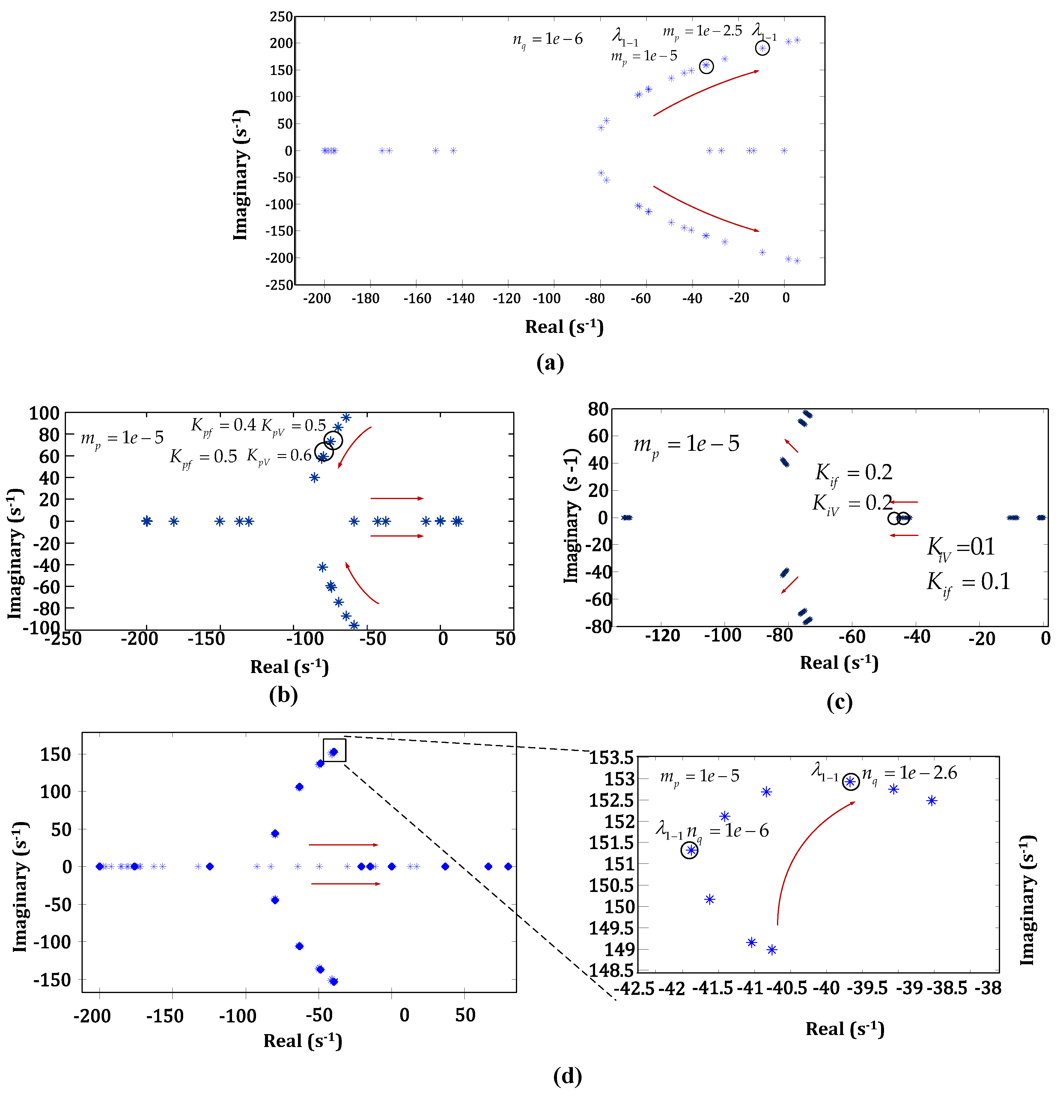
7. Stability and Sensitivity Analysis

The small signal model of the MG given by Equations (48)–(53) is utilized to plot eigen values of the system under varying control and system parameters. Eigen values or modes are solutions to characteristic equation of the system’s linearized state matrix. Sensitivity of the system states to changes in system parameters can be determined by analyzing the system state matrix A_MG. A sensitivity factor rp_ki gives the measure of association between different state variables and their participation in modes [36,39]. Sensitivity, rp_ki of an eigen value λ_i, in relation to the corresponding diagonal element of state matrix a_kk, can be given by (56):

$$r{p}_{ki}=\frac{\partial {\lambda }_i}{\partial a_{kk}}$$

(56)

Eigen evolution traces are plotted to perform stability and sensitivity analyses, ascertain limits for the test MG network under the proposed control scheme. The droop gains of all inverters as well as multiagent consensus gains have been perturbed to arrive at operational limits of the system as given in

Table 4. Variation range for primary and secondary controller gains.

Sr. No.	Control Parameters
1.	Droop Gains	Min.	Max.
	mp	1 × 10−10	1 × 10−3
	nq	1 × 10−7	1 × 10−3
2.	Consensus frequency
	kpf	0.4	2.5
	kif	0.1	0.6
3.	Consensus voltage
	kpV	0.5	3.5
	kiV	0.1	0.7

. Eigen traces given in Figure 4a–d demonstrate system behavior under varying control gains. Figure 4a shows the movement of eigen values with increase in m_p, towards the right half plane. Figure 4b shows the movement of eigen values under influence of increasing proportional consensus gains, (K_pV, K_pf), towards the right half plane. Figure 4c shows the movement of eigen values under influence of increasing integral consensus gains, (K_iV, K_if) towards the left half of the plane. Proportional consensus gains (K_pV, K_pf) tend to force the system towards early convergence, however they push the system stability to its limits. Conversely, integral consensus gains (K_iV, K_if) tend to stabilize the system. Figure 4d shows the movement of poles under influence of increasing reactive power control gains n_q, towards the right half plane_. Table 4 gives operational limits of control parameters obtained from the analysis. Overall, the MG system is more sensitive towards variation in reactive power control gains n_q than active power gains m_p.

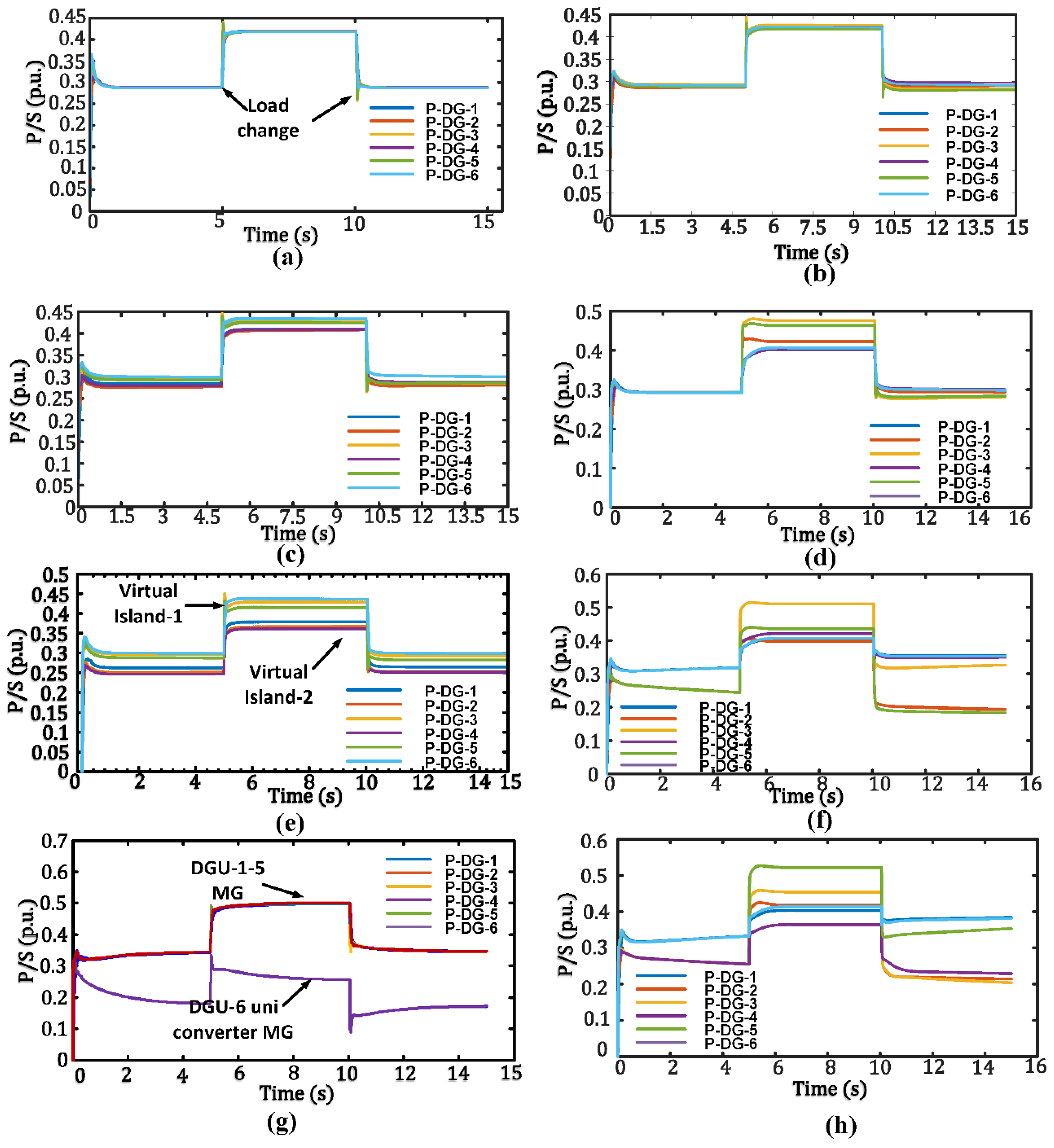
8. Evaluation with Case Studies

This section elaborates case study simulations undertaken for scenarios resulting from multiple communication link failures. The proposed algorithm subsequently segments the microgrid network into “virtual sub islands” described as follows. Figure 5a–g gives active power sharing results for each case discussed.

8.1. Case-1: Full Ring Sparse Connected Communication Network

In the first scenario considered, the communication network between nodes forms a complete ring digraph as represented in Figure 3a. All nodes receive information from neighboring nodes and, as such, no communication islands are formed. All converter nodes converge to proportional values of active power injection as seen in Figure 5a.

8.2. Case-2: Two Sub Groups with Equal Number of Members

This scenario is based on multiple link failures leading to the segmentation of the microgrid communication network into two virtual islands of approximately equal size. The DGUs 1 through 3 form one communication sub-island whereas DGUs 4 through 6 form another sub-island as shown in Figure 3b. Subsequently, with the aid of proposed controls, active power injected by all nodes falls within two subgroups as can be seen Figure 5c, whereas, in absence thereof, the injected powers diverge, as seen in Figure 5e.

8.3. Case-3: Three or More Sub Groups with Equal Number of Members

This considers a scenario where communication link failures divide the microgrid information network into three or more virtual sub-islands approximately equal in size viz the number of nodes in each. Accordingly, DGUs 1 and 2, 3 and 4, 5 and 6, form three virtual sub islands as shown in Figure 3c. The control algorithms within each sub-island drive the system to achieve proportional power sharing as shown in Figure 5e. Conversely, Figure 5c shows an imbalance in injected active powers when the proposed tertiary controls are absent.

8.4. Case-4: Two Sub Groups with Un-Equal Number of Members

This scenario considers an event wherein one node becomes completely isolated from the other nodes due to multiple communication link failures. The DGUs 1 through 5 correspond to one virtual sub-island. Whereas, the DGU-6 is isolated as an individual converter sub-island as shown in Figure 3d. The results obtained for this can be seen in Figure 5g. It may be observed that tertiary controls enable the power injected to fall within two subgroups accordingly, whereas, in absence thereof, the injected powers diverge.

8.5. Comparison with Previous Conventional Control Strategies

Figure 5 compares the simulation study results obtained for the proposed control strategy with results of conventional consensus-based control and distributed estimation-based methods. The left half of the figure (Figure 5: (a) (c) (e) (g)) shows the results for the proposed method, whereas, those on the right (Figure 5: (b) (d) (f) (h)) are the results of consensus-based control. It can be observed that for all cases presented, the proposed method shows better convergence than previously existing control schemes. Figure 6a,b present results for frequency and voltage restoration with the proposed control strategy, whereas, subfigures (c) and (d) present results of frequency and voltage restoration with consensus-based control under faulted communication links.

Table 5. Comparison of the proposed control strategy with existing conventional Strategies.

Sr. No.	Parameters	Proposed Method	Distributed Estimation-Based Methods [22,25,26]	Consensus-Based Methods [12,20,21,23]
1.	Maximum Active power mismatch	0.03 p.u.	0.05 p.u.	0.10 p.u.
2.	Max Voltage variation	0.01 p.u.	0.1 p.u.	0.2 p.u.
3.	Max frequency variation	0.4 Hz (4.0 × 10−5 Hz/VA)	0.2 Hz (2.0 × 10−5 Hz/VA)	1 Hz (1.0 × 10−5 Hz/VA)
4.	Convergence time (frequency)	4 s	10 s	No convergence if links severed
5.	Convergence time (voltage)	1 s	7 s	No convergence if links severed

compares the proposed strategy with conventional methods previously discussed under similar testing circumstances following respective details presented. The proposed method shows early convergence under a given condition as compared with others with lesser active power mismatch between DGUs.

9. Conclusions

A hierarchical multiagent consensus-based control strategy is proposed to address the coupled objectives of power balancing between generation sources, voltage and frequency restoration in islanded AC microgrids. A sparse communication network spans alongside a system distribution network and provides media for communication of estimated values and corrective signals. The proposed method mitigates system instability and power sharing imbalances when the supervisory communication network is experiencing link failures. The nodes lying inside connected communication neighborhoods form virtual “sub-islands”, wherein, power sharing, voltage and frequency regulation control function with reference to locally available information. To verify the effectiveness of the proposed strategy, mathematical small signal models of individual components are stitched together to form an MG system model. These models are then used to analyze the performance of the said controls using eigen plots with regards to system stability and sensitivity towards variation in control parameters. Case simulation studies for different communication scenarios are undertaken. The two kinds of analyses adopted verify the effectiveness of the proposed control strategy for the given scenarios.

References

1. Zeng, Z.; Yang, H.; Zhao, R. Study on small signal stability of microgrids: A review and a new approach. Renew. Sustain. Energy Rev. 2011, 15, 4818–4828. [Google Scholar] [CrossRef]
2. Han, Y.; Li, H.; Shen, P.; Coelho, E.A.A.; Guerrero, J.M. Review of active and reactive power sharing strategies in hierarchical controlled microgrids. IEEE Trans. Power Electron. 2017, 32, 2427–2451. [Google Scholar] [CrossRef]
3. Habib, S.; Kamran, M.; Rashid, U. Impact analysis of vehicle-to-grid technology and charging strategies of electric vehicles on distribution networks—A review. J. Power Sources 2015, 277, 205–214. [Google Scholar] [CrossRef]
4. Hossain, M.A.; Pota, H.R.; Issa, W.; Hossain, M.J. Overview of AC microgrid controls with inverter-interfaced generations. Energies 2017, 10, 1300. [Google Scholar] [CrossRef]
5. Guerrero, J.M.; Matas, J.; de Vicuna, L.G.; Castilla, M.; Miret, J. Decentralized control for parallel operation of distributed generation inverters using resistive output impedance. IEEE Trans. Ind. Electron. 2007, 54, 994–1004. [Google Scholar] [CrossRef]
6. Guerrero, J.M.; De Vicuña, L.G.; Matas, J.; Miret, J.; Castilla, M. Output impedance design of parallel-connected UPS inverters. IEEE Int. Symp. Ind. Electron. 2004, 2, 1123–1128. [Google Scholar] [CrossRef]
7. Guerrero, J.M.; Matas, J.; De Vicuña, L.G.; Castilla, M.; Miret, J. Wireless-control strategy for parallel operation of distributed-generation inverters. IEEE Trans. Ind. Electron. 2006, 53, 1461–1470. [Google Scholar] [CrossRef]
8. Guerrero, J.M.; Vásquez, J.C.; Matas, J.; Castilla, M.; García de Vicuna, L. Control strategy for flexible microgrid-based on parallel line-interactive UPS systems. IEEE Trans. Ind. Electron. 2009, 56, 726–736. [Google Scholar] [CrossRef]
9. De Brabandere, K.; Bolsens, B.; Van Den Keybus, J.; Woyte, A.; Driesen, J.; Belmans, R. A voltage and frequency droop control method for parallel inverters. IEEE Trans. Power Electron. 2007, 4, 1107–1115. [Google Scholar] [CrossRef]
10. Han, H.; Hou, X.; Yang, J.; Wu, J.; Su, M.; Guerrero, J.M. Review of power sharing control strategies for islanding operation of AC microgrids. IEEE Trans. Smart Grid 2016, 7, 200–215. [Google Scholar] [CrossRef]
11. Guerrero, J.M.; Chandorkar, M.; Lee, T.L.; Loh, P.C. Advanced control architectures for intelligent microgridspart I: Decentralized and hierarchical control. IEEE Trans. Ind. Electron. 2013, 60, 1254–1262. [Google Scholar] [CrossRef]
12. Bidram, A.; Member, S.; Davoudi, A.; Lewis, F.L.; Guerrero, J.M.; Member, S. Distributed cooperative secondary control of microgrids using feedback linearization. IEEE Trans. Power Syst. 2013, 28, 3462–3470. [Google Scholar] [CrossRef]
13. Kordkheili, H.; Banejad, M.; Kalat, A.; Pouresmaeil, E.; Catalão, J. Direct-lyapunov-based control scheme for voltage regulation in a three-phase islanded microgrid with renewable energy sources. Energies 2018, 11, 1161. [Google Scholar] [CrossRef]
14. Han, H.; Li, L.; Wang, L.; Su, M.; Zhao, Y.; Guerrero, J.M. A novel decentralized economic operation in islanded AC microgrids. Energies 2017, 10, 804. [Google Scholar] [CrossRef]
15. Lu, L.Y.; Chu, C.C. Consensus-based secondary frequency and voltage droop control of virtual synchronous generators for isolated AC micro-grids. IEEE J. Emerg. Sel. Top. Circuits Syst. 2015, 5, 443–455. [Google Scholar] [CrossRef]
16. Wang, X.; Zhang, H.; Li, C. Distributed finite-time cooperative control of droop-controlled microgrids under switching topology. IET Renew. Power Gener. 2017, 11, 707–714. [Google Scholar] [CrossRef]
17. Wang, H.; Zeng, G.; Dai, Y.; Bi, D.; Sun, J.; Xie, X. Design of a Fractional Order Frequency PID Controller for an Islanded Microgrid : A multi-objective extremal optimization mathod. Energies 2017, 10, 1502. [Google Scholar] [CrossRef]
18. Lewis, F.L.; Qu, Z.; Davoudi, A.; Bidram, A. Secondary control of microgrids based on distributed cooperative control of multi-agent systems. IET Gener. Transm. Distrib. 2013, 7, 822–831. [Google Scholar] [CrossRef]
19. Liu, W.; Gu, W.; Xu, Y.; Wang, Y.; Zhang, K. General distributed secondary control for multi-microgrids with both PQ-controlled and droop-controlled distributed generators. IET Gener. Transm. Distrib. 2017, 11, 707–718. [Google Scholar] [CrossRef]
20. Zuo, S.; Davoudi, A.; Song, Y.; Lewis, F.L. Distributed finite-time voltage and frequency restoration in islanded AC microgrids. IEEE Trans. Ind. Electron. 2016, 63, 5988–5997. [Google Scholar] [CrossRef]
21. Guo, F.; Wen, C.; Mao, J.; Song, Y.D. Distributed secondary voltage and frequency restoration control of droop-controlled inverter-based microgrids. IEEE Trans. Ind. Electron. 2015, 62, 4355–4364. [Google Scholar] [CrossRef]
22. Lu, X.; Yu, X.; Lai, J.; Guerrero, J.M.; Zhou, H. Distributed secondary voltage and frequency control for islanded microgrids with uncertain communication Links. IEEE Trans. Ind. Inform. 2017, 13, 448–460. [Google Scholar] [CrossRef] [Green Version]
23. Wang, Y.; Wang, X.; Chen, Z.; Blaabjerg, F. Distributed optimal control of reactive power and voltage in islanded microgrids. IEEE Trans. Ind. Appl. 2017, 53, 340–349. [Google Scholar] [CrossRef]
24. Schiffer, J.; Seel, T.; Raisch, J.; Sezi, T. Voltage stability and reactive power sharing in inverter-based microgrids with consensus-based distributed voltage control. IEEE Trans. Control Syst. Technol. 2016, 24, 96–109. [Google Scholar] [CrossRef]
25. Guan, Y.; Meng, L.; Li, C.; Vasquez, J.; Guerrero, J. A dynamic consensus algorithm to adjust virtual impedance loops for discharge rate balancing of AC microgrid energy storage units. IEEE Trans. Smart Grid 2017, 3053. [Google Scholar] [CrossRef]
26. Bidram, A.; Nasirian, V.; Davoudi, A.; Lewis, F.L. Droop-free distributed control of AC microgrids. Adv. Ind. Control 2017, 31, 141–171. [Google Scholar] [CrossRef]
27. Guerrero, J.M.; Vasquez, J.C.; Matas, J.; De Vicuña, L.G.; Castilla, M. Hierarchical control of droop-controlled AC and DC microgrids - A general approach toward standardization. IEEE Trans. Ind. Electron. 2011, 58, 158–172. [Google Scholar] [CrossRef]
28. Bidram, A.; Nasirian, V.; Davoudi, A.; Lewis, F.L. Cooperative Synchronization in Distributed Microgrid Control, 1st ed.; Grimble, M.J., Ed.; Springer International Publishing: Basel, Switzerland, 2017; ISBN 978-3-319-50807-8. [Google Scholar]
29. Coelho, E.A.A.; Wu, D.; Guerrero, J.M.; Vasquez, J.C.; Dragičević, T.; Stefanović, Č.; Popovski, P. Small-Signal Analysis of the Microgrid Secondary Control Considering a Communication Time Delay. IEEE Trans. Ind. Electron. 2016, 63, 6257–6269. [Google Scholar] [CrossRef] [Green Version]
30. Char, J.P. Circuit, cutset and path enumeration, and other applications of edge-numbering convention. Proc. Inst. Electr. Eng. 1970, 117, 532–538. [Google Scholar] [CrossRef]
31. Char, J.P. Generation and realisation of loop and cutsets. Proc. Inst. Electr. Eng. 1969, 116, 2001–2008. [Google Scholar] [CrossRef]
32. Gibbons, A. Algoritmic Grpah Theory; Cambridge Univeristy Press: Cambridge, UK, 1985. [Google Scholar]
33. Egerstedt, M.; Mesbahi, M. Graph Theoretic Method in Multiagent Networks; Princeton University Press: Princeton, NJ, USA, 2010; ISBN 9780691140612. [Google Scholar]
34. Lewis, F.L.; Zhang, H.; Hengster-Movric, K.; Das, A. Cooperative Control of Multi Agent Systems, 1st ed.; Springer International Publishing: Basel, Switzerland, 2014; Volume 53, ISBN 9781447155737. [Google Scholar]
35. Lee, K.K.; Chen, C.E. An Eigen-based approach for enhancing matrix inversion approximation in massive MIMO systems. IEEE Trans. Veh. Technol. 2017, 66, 5483–5487. [Google Scholar] [CrossRef]
36. Mahmoud, M.S.; AL-Sunni, F.M. Control and Optimization of Distributed Generation Systems, 1st ed.; Springer International Publishing: Basel, Switzerland, 2015; ISBN 978-3-319-16909-5. [Google Scholar]
37. Pogaku, N.; Prodanović, M.; Green, T.C. Modeling, analysis and testing of autonomous operation of an inverter-based microgrid. IEEE Trans. Power Electron. 2007, 22, 613–625. [Google Scholar] [CrossRef]
38. Yu, K.; Ai, Q.; Wang, S.; Ni, J.; Lv, T. Analysis and optimization of droop controller for microgrid system based on small-signal dynamic model. IEEE Trans. Smart Grid 2016, 7, 695–705. [Google Scholar] [CrossRef]
39. Chen, C.-T. Linear System Theory and Design, 3rd ed.; Oxford University Press: New York, NY, USA, 1999; ISBN 0195117778. [Google Scholar]
Figure 1. Distribution network and control system layout.
Electronics 07 00105 g001
Figure 2. (a) Voltage Control loop; (b) Current Control loop; (c) Primary Control: Power Controller; (d) Secondary Control: Voltage and Frequency regulation.
Electronics 07 00105 g002aElectronics 07 00105 g002b
Figure 3. Communication network connectivity: (a) Full ring bidirectional connectivity; (b) Dual link failure resulting in two symmetrical sub networks; (c) Triple link failure resulting in three symmetrical sub networks; (d) Dual link failure resulting in two asymmetrical sub-networks.
Electronics 07 00105 g003
Figure 4. Observing effect of control gain variation on system stability through eigen traces: (a) effect of variation in mp; (b) effect of variation in tertiary controller integral gains; (c) effect of variation in tertiary controller proportional gains; (d) effect of variation in nq.
Electronics 07 00105 g004
Figure 5. Comparison of active power sharing under proposed control strategy and conventional consensus-based control with varying communication network health: (a) Full ring connectivity with proposed control; (b) Full ring connectivity with consensus-based control; (c) Triple link failure, three sub-islands with proposed control; (d) Triple link failure, three sub islands with consensus-based control (e) Dual link failure, two sub islands with proposed control (f) Dual link failure, two sub islands with conventional consensus-based control (g) Dual link failure, two asymmetrical sub islands with proposed control (h) Dual link failure, two asymmetrical sub islands with consensus-based control.
Electronics 07 00105 g005
Figure 6. System performance under communication failures: (a) Frequency restoration with the proposed control strategy; (b) Voltage restoration with the proposed control strategy; (c) Frequency restoration with consensus-based control; (d) Voltage restoration with consensus-based control.
Electronics 07 00105 g006