Implementation of Deep Learning-Based Automatic Modulation Classifier on FPGA SDR Platform


Guangxi Key Laboratory of Wireless Broadband Communication and Signal Processing, Guilin University of Electronic Technology, Guilin 541004, China
*
Author to whom correspondence should be addressed.
Electronics 2018, 7(7), 122; https://doi.org/10.3390/electronics7070122
Submission received: 3 June 2018
/
Revised: 13 July 2018
/
Accepted: 16 July 2018
/
Published: 19 July 2018
Abstract
:Intelligent radios collect information by sensing signals within the radio spectrum, and the automatic modulation recognition (AMR) of signals is one of their most challenging tasks. Although the result of a modulation classification based on a deep neural network is better, the training of the neural network requires complicated calculations and expensive hardware. Therefore, in this paper, we propose a master–slave AMR architecture using the reconfigurability of field-programmable gate arrays (FPGAs). First, we discuss the method of building AMR, by using a stack convolution autoencoder (CAE), and analyze the principles of training and classification. Then, on the basis of the radiofrequency network-on-chip architecture, the constraint conditions of AMR in FPGA are proposed from the aspects of computing optimization and memory access optimization. The experimental results not only demonstrated that AMR-based CAEs worked correctly, but also showed that AMR based on neural networks could be implemented on FPGAs, with the potential for dynamic spectrum allocation and cognitive radio systems.
1. Introduction
Intelligent radios collect information by sensing signals within the radio spectrum, including the presence, type, and location of the signals. This capability not only identifies friendly or hostile signals in military applications, but also helps regulators to detect whether the use of the radio equipment complies with the spectrum rules. In both cases, an intelligent radio is allowed to take countermeasures corresponding to the perceived information.
In recent years, the application of intelligent radio technology in commercial communications has been defined as software-defined radio (SDR) and cognitive radio (CR) [1,2]. On software and hardware platforms under software control, an SDR can select its operating parameters, including modulation format, coding scheme, antenna configuration, and bandwidth. Therefore, the receiver needs to have a robust method to identify these parameters. CR, by means of opportunities, utilizes the available spectrum of the existing users to provide a solution to the problem of insufficient spectrum utilization [2]. Therefore, one of the key tasks of CR is spectrum sensing [3], which collects information in spectrum scenarios. This information needs to be able to evaluate the possibility of interference with other users and set the corresponding operating parameters. There are plans to allocate the unused spectrum to television broadcasting services through CR.
Signal recognition is a challenging and critical task for intelligent radios. First, the recognition algorithm needs to be able to flexibly sense different signal types under different conditions. For example, primary users with different sensitivity requirements, different transmission rates, and different modulation methods. Second, the recognition algorithm should minimize the requirement for signal preprocessing. For example, these algorithms should not rely on carrier synchronization and channel estimation, because the smart receiver is not synchronized with the perceived radio signal and there is no a priori knowledge of the signal parameters. Finally, even at low signal-to-noise ratios (SNR), the recognition algorithm can provide higher performance with lower complexity in shorter observation time.
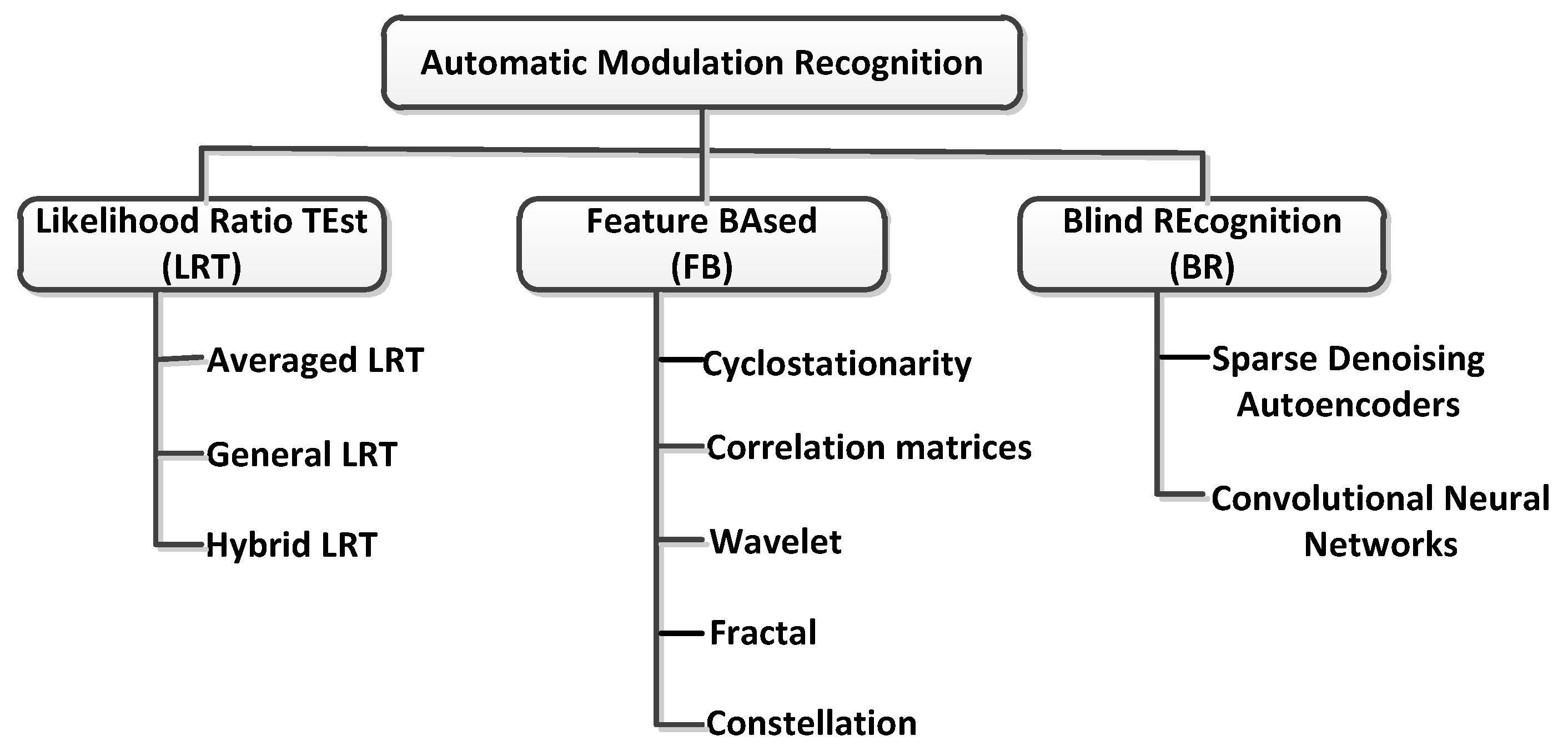
Automatic signal modulation recognition (AMR) is a major research direction of signal recognition. At present, AMR is implemented using the three types of methods listed in Figure 1: (1) The first method is based on the likelihood ratio test (LRT), such as the average LRT proposed by El-Mahdy et al. [4], the general LRT proposed by Panagiotou et al. [5], and the hybrid LRT proposed by Hameed et al. [6]. The disadvantage of this type of algorithm is that the assumption that the symbols are independent and identically distributed is usually not true in reality, and the complexity increases with an increase in the number of unknown parameters. In addition, this type of method is more sensitive to the mismatch of the model; for example, when a time shift occurs, the recognition performance deteriorates considerably; (2) The second method is a feature-based (FB) method that relies on prior knowledge. The features for classification include Dobre’s use of first-order cyclostationary features of digital signals [7] and second-order cyclostationarity [8], the space–time correlation matrix features proposed by Marey and Choqueuse [9,10], wavelet features proposed by Hassan [11], and constellation features proposed by Mobasseri [12]. This method can obtain better results under the condition of a low SNR, but it is necessary to calculate various feature quantities according to the mathematical model of the modulation method in advance, and the calculation method is relatively complicated. In addition, some feature quantities are not complete. For example, the cyclic statistics of signals, such as single-carrier linear digital modulation, orthogonal frequency division multiplexing, and single-carrier frequency domain equalization, have even-order cyclostationarity. Therefore, there are certain restrictions when dealing with signals of these unknown modulation modes; (3) The third method includes blind recognition methods that do not rely on prior knowledge. For example, Migliori’s method of recurrent neural network autoencoder [13] and the convolutional neural network method proposed by O’Shea [14]. Such methods do not need to know the modulation mathematical model of the signal [15]. However, finding a suitable neural network structure requires proficiency in artificial intelligence.
Although the neural network-based modulation classification results presented in [13,14] are better, neural network training is a computationally intensive task. Computers that handle large amounts of radiofrequency (RF) data are expensive, and their size and power consumption do not meet the requirements of portable applications. To this end, we propose the following novel solutions:
- A new structure of AMR based on a stacked convolution autoencoder is proposed [16]. The purpose of neural networks is to approximate the transformation function from the input layer to output layer. Compared with neural networks, the autoencoder can obtain the sparse feature of the signal automatically. The stacked autoencoders can learn multiple expressions of the original data layer by layer. Each layer is based on the expression of the bottom layer, but is often more abstract and more suitable for complex tasks such as classification. Compared with the LRT method, it is no longer necessary to spend a lot of work to build a signal, noise model, and a cost function. Moreover, the randomness of the channel environment makes these models vulnerable to failure. Compared with FB’s method, this method can automatically generate signal characteristics. This feature is suitable for some special occasions, particularly military communications. Because the waveform of the signal in these cases is often non-standard and time-varying in time, frequency and the other domains, the signal characteristics are difficult to predict.
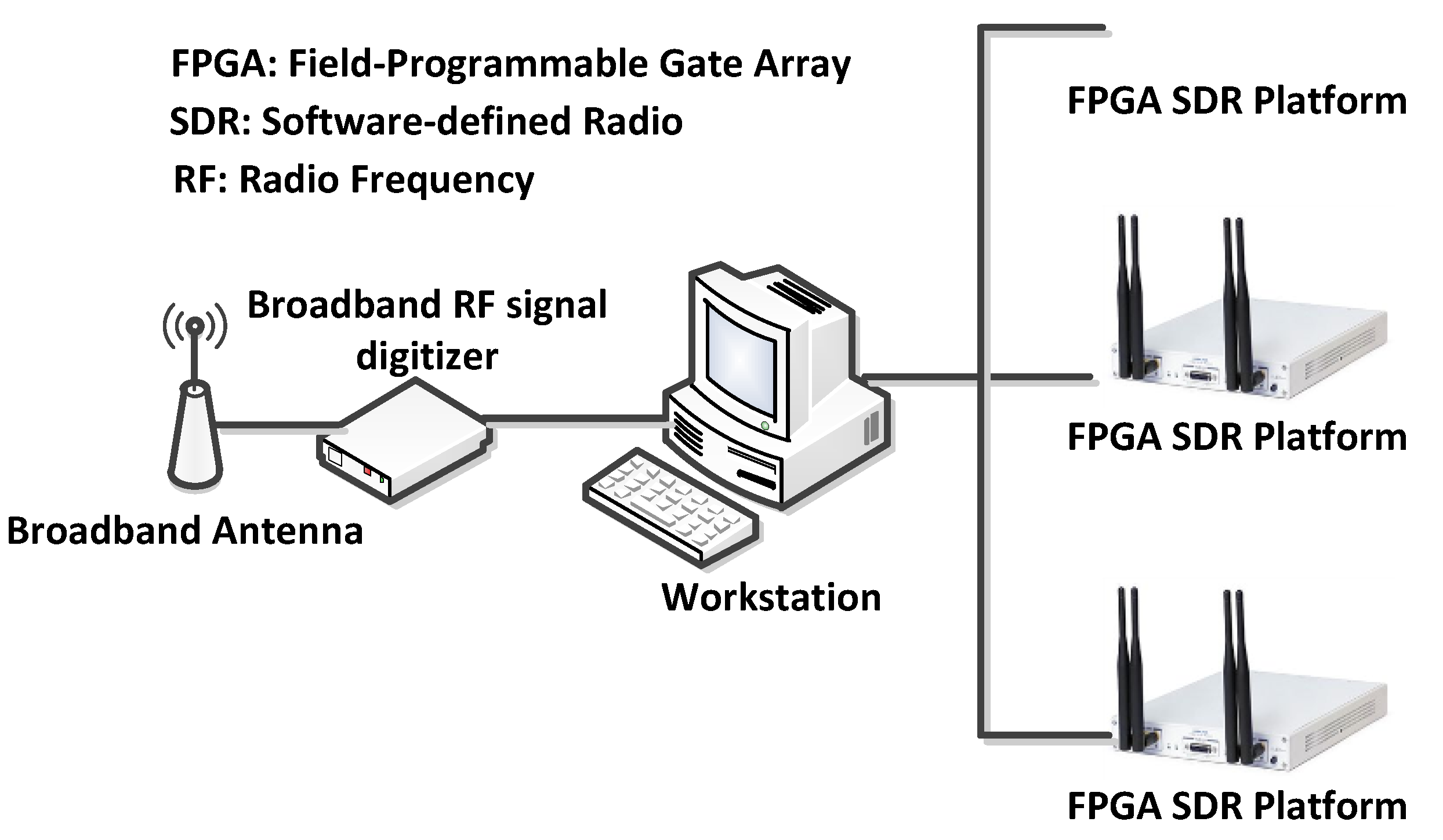
- We used the reconfigurability of field-programmable gate arrays (FPGA) to propose a master–slave AMR architecture. In this architecture, shown in Figure 2, the deep neural network setup and training tasks are performed on a workstation equipped with a graphics processing unit. First, the RF signal digitizer converts the modulated RF signal to sampled data and enters the workstation for training the network. After completing the neural network training, it is converted to the FPGA hardware configuration file on the workstation. Finally, the hardware configuration file is transmitted to the FPGA SDR platform by wireless or wired communication, updating the configuration of the AMR function. The trained hardware model can be operated on portable radio equipment, thus reducing the requirements of hardware. If there is a new type of modulation that needs to be identified, the system needs to be retrained. After the training is completed, new weights are generated. At this time, the original FPGA fabric needs to be updated. Therefore, reconfigurability is necessary for the evolution of the system. The current AMR is not reconfigurable, so no recognition can be made for the new modulation type. With respect to such a situation, the proposed scheme adds value to the actual project. This is also a very important function for identifying non-standard and time-varying signals in multiple domains. As a large number of intelligent radio terminals can share the training results of a workstation, the computational costs can be decreased considerably.
The rest of this paper is organized as follows. In the next section, the principle of the modulation classification of radio signals is analyzed, and a modulation classifier structure using convolutional autoencoders (CAEs) is proposed. In Section 3, we discuss how to convert a trained neural network model into an FPGA hardware function module. The experimental results of the modulation classification of actual radio signals are provided in Section 4, and the related discussion of the results is presented in Section 5.
2. Construction of Automatic Modulation Recognition
The deep learning method represented by the convolutional network (CNN) [17] adopts the local connection method and the sharing weight method. This reduces the number of parameters, shows superiority in image processing, and is closer to the actual biological neural networks. In addition to reducing the number of parameters, CNN uses feature extraction to avoid the complex pre-processing of the image and can directly input the original image [17]. If the input of the deep neural network is not an image but a sampling of the communication signal, the work carried out in [13] and [14] proves that the signals of different modulation methods can be better classified.
2.1. Problem Description
2.1.1. Signal Characteristics
In digital receivers, the in-phase and quadrature components of the radio signal can be obtained through analog-to-digital conversion, forming a complex-valued vector. The received signal can be expressed as follows:
where is a modulated signal whose frequency, phase, amplitude, etc., are controlled by analog or digital modulation signals. Further, is the channel impulse response function and is the additive noise in the channel. However, Equation (1) is an idealized expression. In practical applications, the following influencing factors of the application are not negligible: the random phase noise of the carrier frequency, the random phase noise of the phase of the sampling clock, the time-varying of the amplitude-frequency and phase-frequency characteristics of the channel corresponding function , the Gaussian nature of additive noise, and so on. These factors are time-varying sources of error. The actual signal is as follows:
Equation (2) shows that the instantaneous phase of the signal is affected by the phase noise of the carrier. The sampling interval of the signal is randomly changed. For an actual communication system, the phase noise of the carrier and the sampling clock should be kept at a fairly low level.
Assuming that the baseband signal is a digital signal, the transmitted information bits are converted into complex baseband signals according to the modulation rules. Then, after the modulation, the voltage of the complex baseband signal is projected onto a sine or cosine function with a carrier frequency of . By controlling the changes in the amplitude, phase, frequency, etc., of the carrier signal, we can modulate the information bits discretely into the space of these parameters during each symbol’s time period. For example, M-QAM’s amplitude, phase mapping is as follows:
where and are discrete amplitude values and . is the number of and . For , .
After the received signals are sampled as discrete I/Q data, they are fed to the neural network for modulation recognition. The data file needs to be arranged in a certain format and structure. The I/Q data is divided into data vectors containing samples. Each data segment is composed of interleaved I and Q values for each sample to form a vector of length . Assume that the number of samples per symbol is . Then, each vector contains symbols. These vectors are placed in two sets for training and testing, respectively (the numbers are and , respectively). In addition, the modulation types and locations in these sets are random. In all of the experiments, the parameter is the same for each modulation type. The specific values of all of the parameters are shown in Table 1.
2.1.2. Recognition of Modulation
Because of the diversity of the modulation methods, the modulation recognition can be seen as an N-class decision problem where the input is a complex time series of received signals. Assuming that a decision system receives the modulated signal , it can output the prediction of the modulation method , where the number of modulation methods is a fixed value, . Let the signal modulated by be —then, the characterization of can use its full joint distribution. Thus, the correct prediction for a given signal can be expressed as follows:
To fully evaluate the performance of , the average of the classification accuracy of the various modulation methods is used:
Of course, is a function of the SNR as the SNR affects the signal. Here, , where is the power of the signal, and is the power of the noise.
2.2. Construction Methods
The neural network used for AMR consists of a series of pre-trained CAEs [16] followed by a fully connected softmax classifier layer. The CAE is just an autoencoder that combines the principles of model design from CNN. This type of model has many applications, including depth feature visualization [17], intensive prediction [18], generative modeling [19,20], and semi-supervised learning [21].
2.2.1. Structure of Stacked CAEs
CAEs filter the input data by using a convolution kernel. In traditional methods, an autoencoder does not take into account the fact that signals can be regarded as the sum of other signals. In contrast, a CAE uses a convolution operation to do so. It filters the input signal to extract part of its content. In the two-dimensional discrete space, convolution operations can be defined as follows:
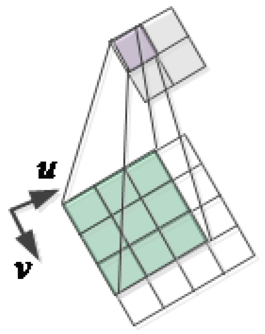
where represents the convolution results of , is an edge of a rectangular odd convolution kernel, is a convolution kernel, and I represents the two-dimensional discrete data of the input. As shown in Figure 3, a convolution kernel is used to convolute the input two-dimensional data I at each location .
CAEs allow model learning to minimize the optimal filter for reconstruction errors, rather than manually designing filters. CAEs are usually used to extract features from input data so as to reconstruct the input data. Due to their convolution property, the number of activation graphs generated by CAEs is the same irrespective of the dimensions of the input data. Therefore, CAEs completely ignore the structure of a two-dimensional image itself, but act as a general feature extractor. Once these convolution kernels are trained and learned, they can be applied to any input data for feature extraction.
A single convolution filter cannot learn to extract various patterns of images. Therefore, each convolutional layer is composed of the convolution kernel with depths of , where represents the number of channels for input data. Therefore, the convolution of each input data element with depth :
and a set of n convolution kernels:
produces a set of activation graphs:
To improve the generalization of the network, each convolution is wrapped with an activation function so that the training process can learn to use the activation function to represent the input:
where represents the deviation of the -th feature map. The resulting activation map is the encoding of the input in the low-dimensional space, the dimensions of which are the number of parameters used to establish each feature map , that is, the number of parameters to learn.
To reconstruct the input data from the generated feature map, a decoding operation is required. The CAE is a complete convolutional network, so the decoding operation can be reconvoluted. Using the generated feature maps as inputs to the decoder, we can reconstruct the input data from the compressed information. Therefore, the reconstructed data are the result of the convolution between the feature map and the convolution filter :
The cost function used to train the neural network is the mean squared error:
For standard networks, a back-propagation algorithm is used to calculate the gradient of the error function of the parameters. This result can be easily obtained with a convolution operation by using the following formula:
where and are the delta of the feature map and the reconstruction data, respectively. The weights are then updated using a stochastic gradient descent method.
In fact, the feature map of an autoencoder can be used as the input of another autoencoder, thus forming a stacked architecture [22]. Let , , and represent the input, hidden, and output units of a single autoencoder, respectively. Then, the process of forward propagation by the entire network from the encoder is performed in accordance with the following formula:
where , and is the input layer.
In our application for radio signal I/Q datasets, a random gradient descent method was used for continuous, unsupervised training of a single autoencoder layer with a batch size of 50. For deep belief networks, unsupervised pre-training can be conducted in a greedy, layered manner [23].
2.2.2. Training and Classification
After the completion of the unsupervised pre-training phase, supervised fine-tuning was carried out. At this stage, we added pre-trained autoencoders to a pure feedforward multi-layer perceptron in the form of Equation (15) and attached a final layer for the classification:
In the multilayer perceptron final output vector as a reflection of the modulation type of probability distribution, L2 regularization item supervised learning was added to minimize the negative logarithm likelihood function, to ensure that the model was in the stage of unsupervised learning sparse activation. The value of a regularized item was set to 1 or 0, depending on the required experimental configuration. Suppose that is a sample list, is the number of layers, is the output of the -th layer, and represents the weight matrix between the -th layer and the ()-th layer. Then, the layer sensor loss function can be expressed as follows:
where ti is the index corresponding to the correct label of sample and is the number of cells in layer . We use the batch stochastic gradient descent method to minimize Equation (14) [24]. The overall architecture of our proposed modulation classifier is shown in Figure 4, and the fixed parameters used in the experiment are listed in Table 2.
3. Implementation
It is very easy to change the architecture of a neural network by using software, but for the hardware, the FPGA fabric cannot be arbitrarily reconfigured. First, a neural network cannot provide a solution that satisfies all the applications. Second, the neural network architecture (size, type, and number of layers) is the main driver of performance, but a generic FPGA solution cannot be created because the various possible architectures are very large. Such a solution either consumes a lot of resources or fails to achieve the desired throughput.
3.1. Architecture
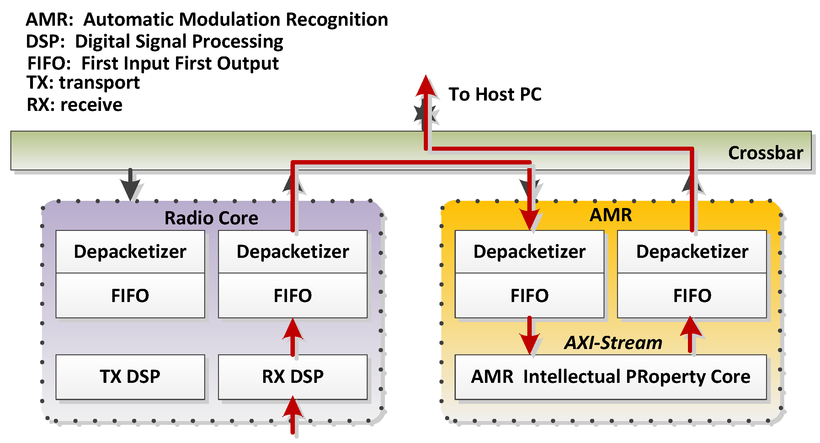
RF network-on-chip (RFNoC) is an open-source framework for developing data processing applications that can be run on FPGAs [25]. It is a method of modularizing signals or data processing components on an FPGA and effectively accessing them. The processing is divided into blocks (or computational engines), and data are passed between blocks. These blocks are connected to a crossbar, which allows the arbitrary routing of packets between arbitrary blocks. RFNoC is responsible for passing data between blocks, routes, and configuration blocks from the software. Data can also be passed back and forth between RFNoC blocks and the software. We can decompose the radio system into different functional blocks, each of which executes a digital signal processing (DSP) algorithm. As shown in Figure 5, the data from the radio are routed to the AMR intellectual property (IP) block proposed herein, and all of the data between the blocks are packed.
Internally, all of the blocks contain a generic framework interface called Noc-Shell [15]. This allows any type of AXI-Stream-compatible IP to be connected to the RFNoC network. Noc-Shell is responsible for packetization, offline, routing, flow control, and any common settings between blocks. By setting the appropriate routing information, Noc-Shell can correctly process all of the transmitted packets so that they can reach the intended destination.
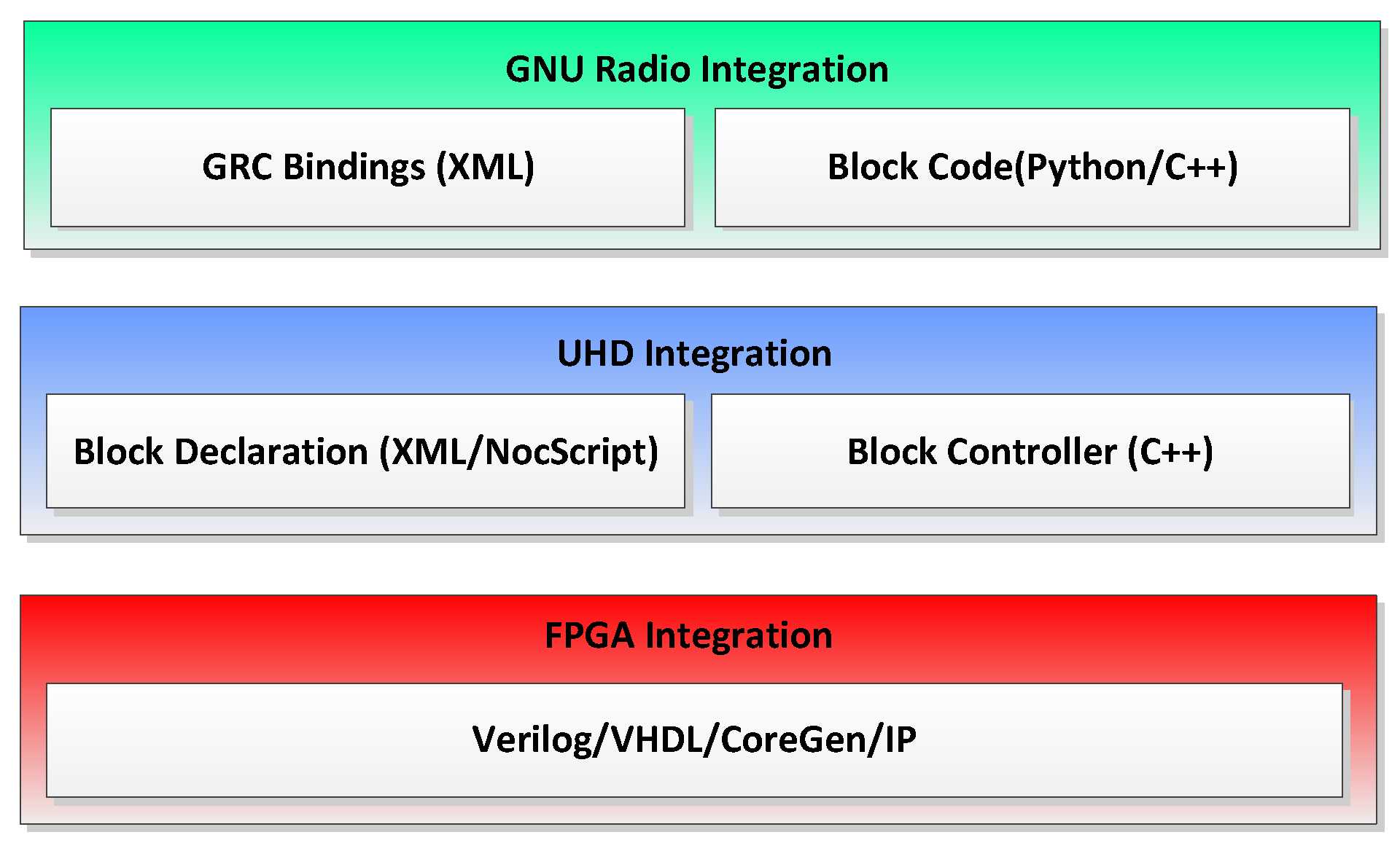
As shown in Figure 6, the components of the RFNoC module have three levels of content, including its integration with GNU Radio. In a nutshell, the development work needed for these three levels is as follows:
1. The actual FPGA IP. This is the main part of the development work and includes various DSP algorithms, modulation, demodulation, carrier synchronization, and so on.
2. Block control. To control the blocks from the software, some host driver code needs to be written.
3. GNU Radio integration (or integration into other frameworks). According to the actual application requirements, determine whether this step is needed.
RFNoC is not only an extension of the SDR tool, but can also be used alone to build a modular SDR application running on an FPGA. It provides a reliable, modular transport layer between the FPGA and the processor so that different hardware platforms can use the exact same RFNoC FPGA and software code, while RFNoC handles the FPGA-to-processor interface. In addition, any aspect of the software interface specific to an RFNoC calculation engine is dynamically connected to the correct FPGA component and is reusable across different hardware platforms.
3.2. AMR IP
Since RFNoC between the hardware and the software provides a convenient input/output interface, our work focuses on the trade-off between the resources and the throughput in the neural network, without the need for software development, the maintenance of the FPGA, and the repetitive glue code. On the premise that its structure has been determined, we adopt the Vivado HLS tool of Xilinx to implement the FPGA IP of the neural network shown in Figure 4. Vivado HLS is used to synthesize the C, C++, or System C code into verilog or VHDL code. HDL is generated by using “pragma” instructions inserted into the C code (or a separate instruction file) indicating how the HLS compiler synthesizes the algorithm. For the design shown in Figure 4, we developed the roofline model on the basis of a quantitative analysis of different optimization techniques (circulation block and transform), computing throughput, and the required memory bandwidth so as to find the best performance and the lowest FPGA resource demand solutions [26].
The neural network described by the C++ HLS tool was composed of the rectified linear unit function (ReLU), tanh, sigmoid, convolution, maxpool, and so on. We optimized the computations and the memory access according to the design method proposed by Zhang et al. [26].
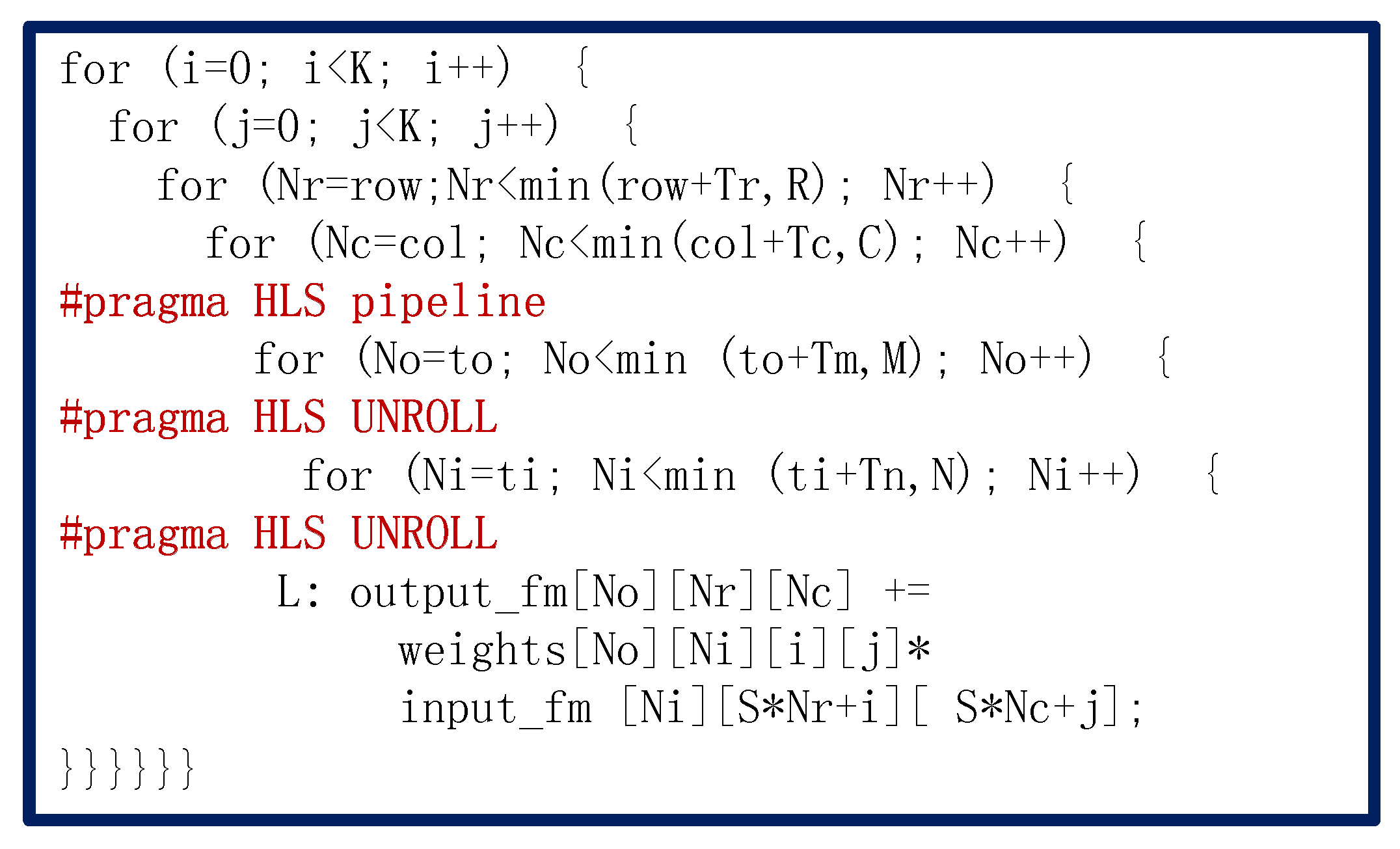
Although a large number of loop operations in the convolution consume considerable computational time, the use of loop blocking can fully utilize the hardware resources in the FPGA to perform parallel processing on the data and accelerate the computations [27]. The example code in C++ HLS is shown in Figure 7. “Circular expansion” can be used to increase the utilization of massive computing resources in FPGA devices. Expanding along different loop dimensions generates different implementation variables. Whether the two deployed execution instances share data and the amount of data shared affect the complexity of the generated hardware and ultimately affect the number of deployed replicas and the frequency of hardware operations. The “circulation pipeline” is a key optimization technique in the high-level synthesis that improves the system throughput by overlapping the execution of operations from different loop iterations. The throughput achieved is limited by the resource constraints and data dependencies in the application. The dependencies carried by the loop will prevent the loop from being completely streamlined.
Memory access optimization is achieved through data reuse. The convolution of CAEs needs to load the input/output feature maps and weights before starting and to write the generated output feature maps back to the main memory. As the neural network is pre-trained, the weights can be solidified into the FPGA. Therefore, the memory access is mainly the input/output of the feature map. If the innermost loop is independent of the array, there are redundant memory operations between different loop iterations. At this point, local memory promotion [28] can be used to reduce redundant operations. To maximize the opportunity for data reuse through local memory promotions, we use a polyhedron-based optimization framework to identify all legal loop transformations.
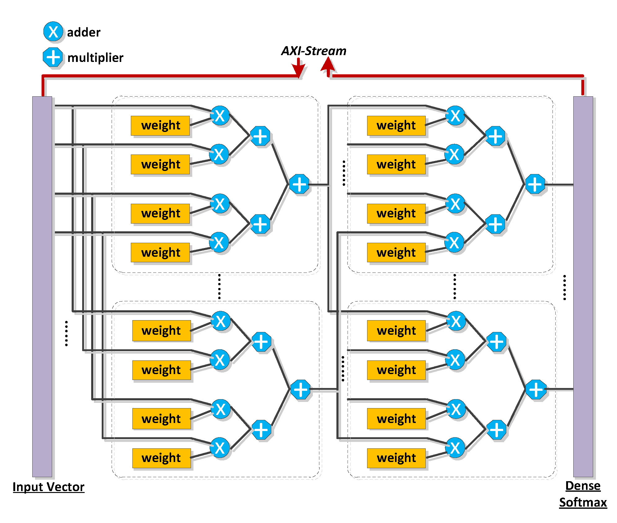
After synthesizing the neural network into the FPGA code through HLS, we packaged it using verilog for secure interactions with the RFNoC architecture. This is also the Noc-Shell described in Section 3.1, which connects the AXI-Stream-compatible neural network IP to the RFNoC network. The structure is shown in Figure 8.
4. Results
4.1. Use of Resources
Through experiments in TensorFlow, we used some of these software components to construct an optimized AMR structure as shown in Figure 4 and Table 2. In the AMR, the total number of weights was 2,830,427. Each weight was a 32-bit fixed-point number and therefore, occupied 90,573,664 bits of storage. We completed the pre-training of the AMR on a workstation with the Xeon E-1600V4 CPU, operating frequency of 3.5 GHZ, and RAM capacity of 16 GB. The operating system used 64-bit Ubuntu 16.04 LTS. No GPU acceleration was used during the training. In the training process, the batch size of the stochastic gradient descent was 1024.
The number of complex samples used for the training was 24 million, and these samples included types of modulation. The samples were divided into 256 training sample sets. We used approximately 93,000 samples for the training. These samples were evenly distributed over the SNR range of −20 dB to +20 dB and were flagged so that we could evaluate the performance of a specific subset. The training process was completed after 39 epochs. The total time required was 15 h and 26 min.
Then, we applied Vivado HLS to generate the AMR hardware code. Table 3 shows the estimates of the resource usage after the hardware code was synthesized, indicating the nominal FPGA results for the relevant component sizes used in the AMR. Although the block-random access memory (BRAM) usage of the fully connected layer was high, the DSP48s module, the flip-flop (FF), and the look-up table (LUT) generally achieved relatively low device utilization.
4.2. Experiment
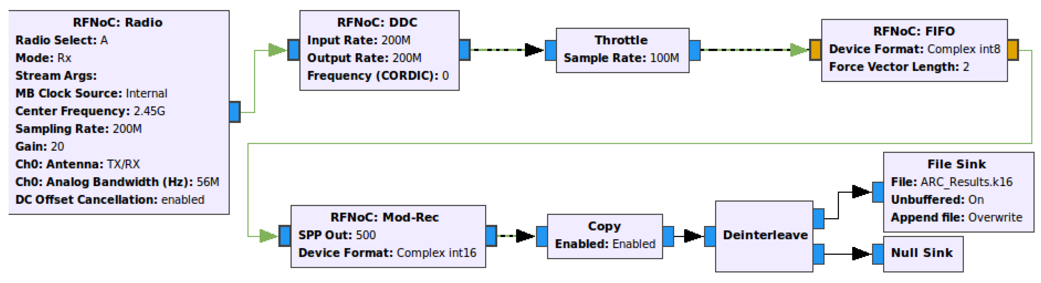
AMR was built into the FPGA image targeted to the Ettus SDR platform by using a workflow that created the RFNoC image. The newly created AMR block did not require a custom C++ driver, but required several XML definitions for use in GNU radio companion (GRC). Once the GRC XML file was ready, the AMR module was inserted into the GRC flowchart for the user input and output (Figure 9) and then run locally or on an Ettus SDR series device.
We used 64,000 samples to test the AMR running on the Ettus X310. When the number of test vectors for each signal was 1000, the time for obtaining the modulation classification result was 3.75 ms.
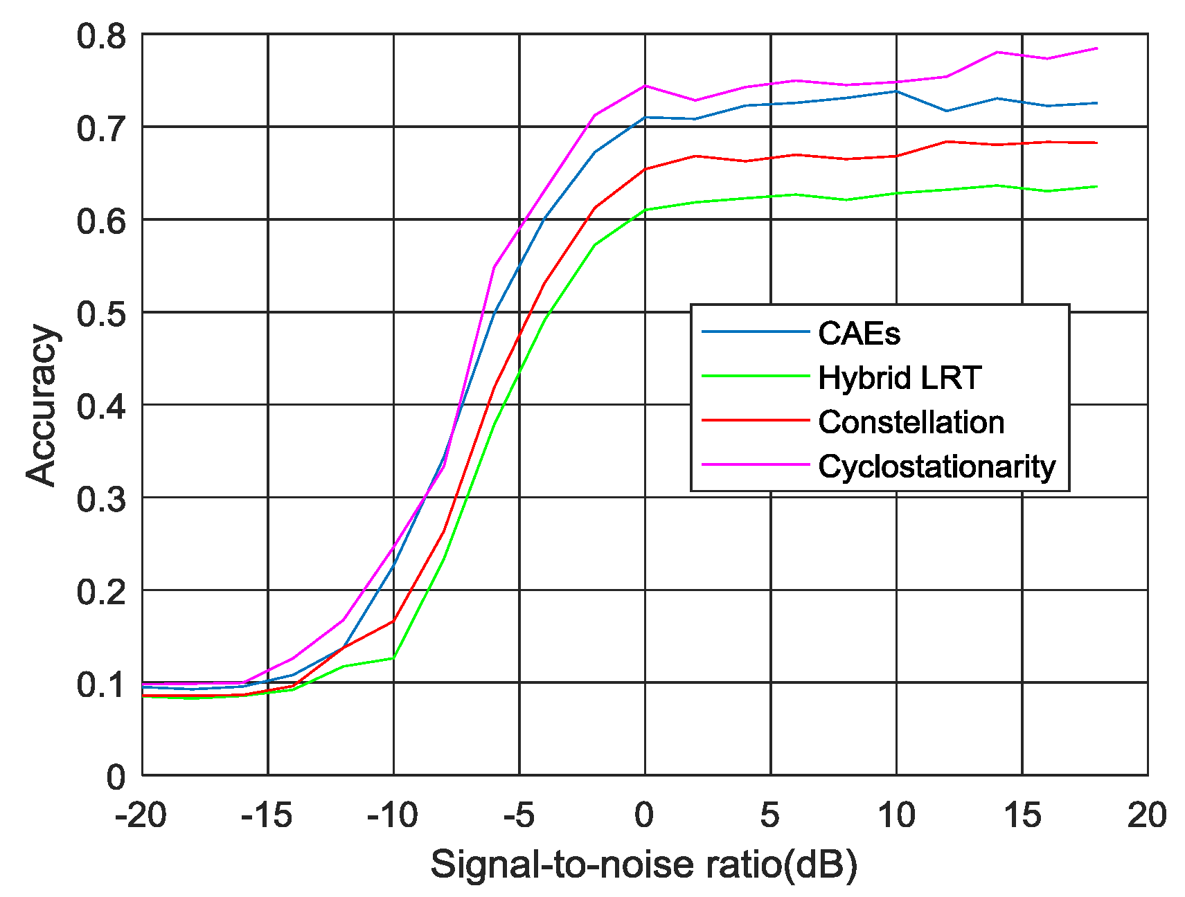
As shown in Figure 10, the experimental results showed that approximately 70%~80% of the average classification accuracy, was achieved for all of the SNRs in the test dataset. The average accuracy of other AMR methods for the same test data is also given in Figure 10.
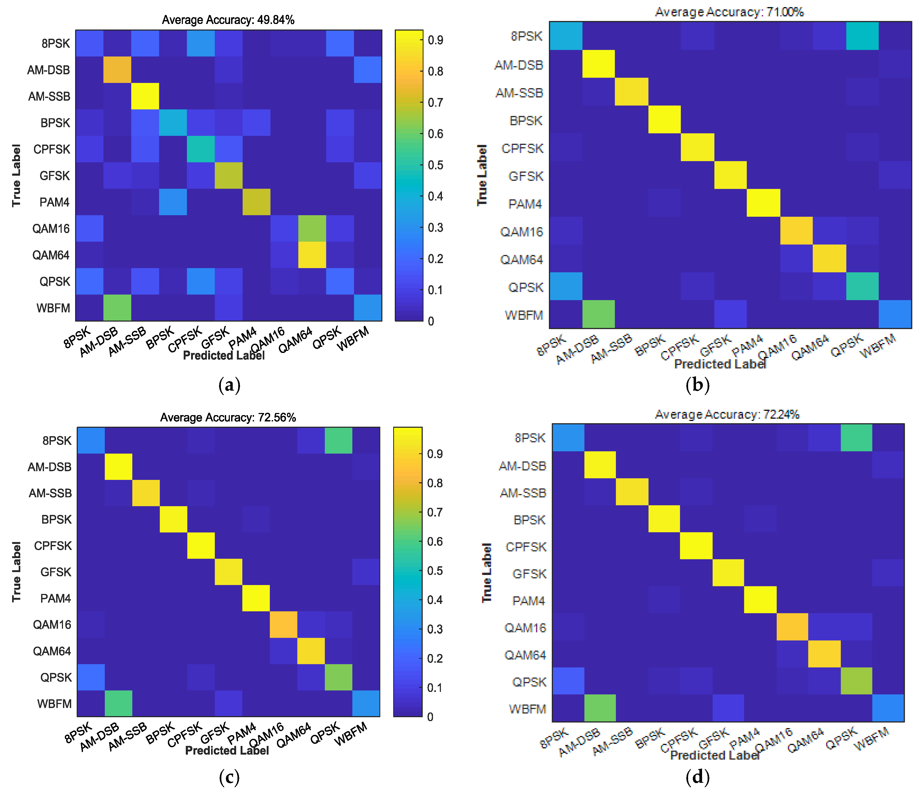
We used the confusion matrix to analyze the probability that the modulation type was misjudged. A confusion matrix is the standard format used for evaluating accuracy. The rows of the matrix represent the instances in a predicted class, while the columns represent the instances in an actual class (or vice versa) [29]. A confusion matrix of dimension consisting of the values of was constructed. The confusion matrices for the AMR with the highest overall performance are shown in Figure 11 at SNRs of −6 dB, 0 dB, 6 dB and 16 dB.
We used the confusion matrix to analyze the probability that the modulation type was misjudged. A confusion matrix is the standard format used for evaluating accuracy. The rows of the matrix represent the instances in a predicted class, while the columns represent the instances in an actual class (or vice versa) [29]. A confusion matrix of dimension consisting of the values of was constructed. The confusion matrices for the AMR with the highest overall performance are shown in Figure 11 at SNRs of −6 dB, 0 dB, 6 dB and 16 dB.
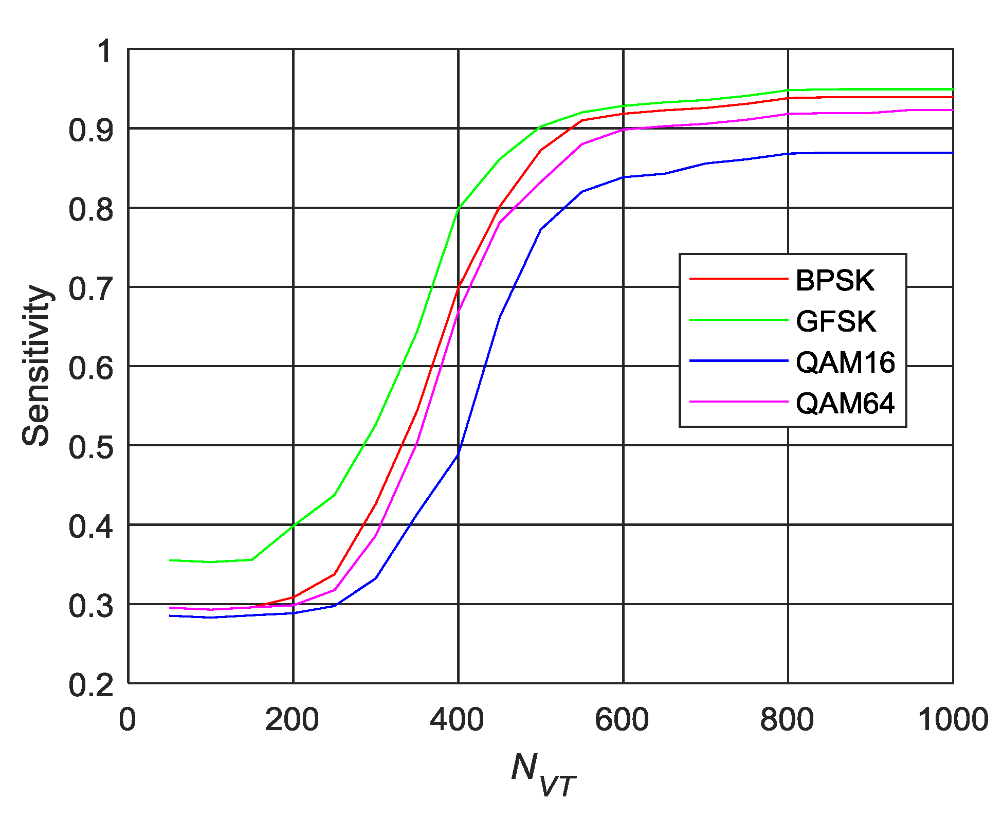
In addition, we also examined the sensitivity of the AMR to each modulation family as a function of the samples. Let and be the true and predicted class label, respectively, for sample i. Then the sensitivity of the AMR for class can be expressed as follows:
where is the indicator function ( if is true and 0 otherwise) and is the number of test vectors. We calculated the sensitivity of BPSK, GFSK, QAM16, and QAM64 with AMR at SNR = 5 dB. The results are shown in Figure 12.
5. Discussion
In this study, we explored a CAE-based automatic modulation classification method and its implementation based on FPGA. This laid the foundation for the deployment of real-time, high-rate, low-power, and useful neural networks for RF communications research and prototyping. The experiments not only proved that the proposed AMR correctly identified most of the modulation types within a wide range of SNR changes and worked better, but they also showed that it was possible to implement AMR on the basis of neural networks on FPGA.
The correct recognition rate as shown in Figure 10 was an average value, ranging from 70% to 80%. It seemed that this result was not as good as feature-based recognition. In practice, however, this average was pulled down by the identification errors of 8PSK and WBFM. Except for these two modulation signals, the correct identification rate of the other modulation types was approximately 90%. Therefore, AMR needs to be improved in a future work to improve the accuracy of the identification of 8PSK and WBFM.
As shown in Figure 11, at an SNR of +18 dB, we obtained a clean diagonal in the confusion matrix. We observed that our remaining difference of 8 PSK was misclassified as QPSK and WBFM was misclassified as AM-DSB. As the QPSK constellation points spanned 8PSK points, 8PSK symbols containing specific bits were difficult to distinguish from QPSK. In the case of WBFM/AM-DSB, there were only carriers during the silence period of the analog speech signal. Therefore, these samples were difficult to identify correctly. Even at high signal-to-noise ratios, we could not achieve 100% accuracy.
The AMR developed in this study could directly identify the modulation type of the radio signal time series, thereby avoiding the computation of cumbersome expert features, and it has the potential for dynamic spectrum allocation and CR systems. On the basis of the implementation of the trained AMR in the FPGA, more neural network algorithms can be added to the FPGA-based SDR system in the future so that the radio equipment has more intelligent applications.
Author Contributions
Conceptualization, Z.-L.T. and S.-M.L.; Methodology, Z.-L.T. and L.-J.Y.; Experiments, Z.-L.T. and L.-J.Y.; Data Analysis, L.-J.Y.; Writing-Original Draft Preparation, Z.-L.T.; Writing-Review & Editing, S.-M.L.
Funding
This work was funded by the National Natural Science Foundation of China under Grant No.61461013, and the Dean Project of Guangxi Key Laboratory of Wireless Broadband Communication and Signal Processing under Grant No.GXKL06160103.
Conflicts of Interest
The authors declare no conflicts of interest.
References
- Xu, J.; Su, W.; Zhou, M. Software-defined radio equipped with rapid modulation recognition. IEEE Trans. Veh. Technol. 2010, 59, 1659–1667. [Google Scholar] [CrossRef]
- Yucek, T.; Arslan, H. A survey of spectrum sensing algorithms for cognitive radio applications. IEEE Commun. Surv. Tutor. 2009, 11, 116–130. [Google Scholar] [CrossRef]
- Dobre, O.A. Signal identification for emerging intelligent radios: classical problems and new challenges. IEEE Instrum. Meas. Mag. 2015, 18, 11–18. [Google Scholar] [CrossRef]
- El-Mahdy, A.; Namazi, N. Classification of Multiple M-ary Frequency-Shift Keying Signals Over a Rayleigh Fading Channel. IEEE Trans. Commun. 2002, 50, 967–974. [Google Scholar] [CrossRef]
- Panagiotou, P.; Anastasoupoulos, A.; Polydoros, A. Likelihood ratio tests for modulation classification. In Proceedings of the 21st Century Military Communications Conference (CMCC 2000), Los Angeles, CA, USA, 22–25 October 2000; pp. 670–674. [Google Scholar]
- Hameed, F.; Dobre, O.A.; Popescu, D.C. On the likelihood-based approach to modulation classification. IEEE Trans. Wirel. Commun. 2009, 8, 5884–5892. [Google Scholar] [CrossRef]
- Dobre, O.A.; Rajan, S.; Inkol, R. Joint signal detection and classification based on first-order cyclostationarity for cognitive radios. EURASIP J. Adv. Signal Process. 2009, 2009, 656719. [Google Scholar] [CrossRef]
- Jerjawi, W.A.; Eldemerdash, Y.A.; Dobre, O.A. Second-Order Cyclostationarity-Based Detection of LTE SC-FDMA Signals for Cognitive Radio Systems. IEEE Trans. Instrum. Meas. 2015, 64, 823–833. [Google Scholar] [CrossRef] [Green Version]
- Choqueuse, V.; Yao, K.; Collin, L.; Burel, G. Hierarchical space-time block code recognition using correlation matrices. IEEE Trans. Wirel. Commun. 2008, 7, 3526–3534. [Google Scholar] [CrossRef] [Green Version]
- Marey, M.; Dobre, O.A.; Inkol, R. Blind STBC identification for multiple antenna OFDM systems. IEEE Trans. Commun. 2014, 62, 1554–1567. [Google Scholar] [CrossRef]
- Hassan, K.; Dayoub, I. Automatic Modulation Recognition Using Wavelet Transform and Neural Networks in Wireless Systems. Eurasip J. Adv. Sig. Proc. 2010, 2010, 532898. [Google Scholar] [CrossRef]
- Mobasseri, B.G. Digital modulation classification using constellation shape. Sig. Proc. 2000, 80, 251–277. [Google Scholar] [CrossRef] [Green Version]
- Migliori, B.; Zeller-Townson, R.; Grady, D.; Gebhardt, D. Biologically Inspired Radio Signal Feature Extraction with Sparse Denoising Autoencoders; Technical Report for Space and Naval Warfare Systems: San Diego, CA, USA, 2016. [Google Scholar]
- O’Shea, T.J.; Corgan, J.; Clancy, T.C. Unsupervised representation learning of structured radio communication signals. In Proceedings of the IEEE 2016 First International Workshop on Sensing, Processing and Learning for Intelligent Machines (SPLINE), Aalborg, Denmark, 6–8 July 2016; pp. 1–5. [Google Scholar]
- Ranzato, M.; Fujie, H.; Boureau, Y.L.; LeCun, Y. Unsupervised Learning of Invariant Feature Hierarchies with Applications to Object Recognition. In Proceedings of the IEEE Conference on Computer Vision and Pattern Recognition, Minneapolis, MN, USA, 17–22 June 2007. [Google Scholar] [CrossRef]
- Masci, J.; Meier, U.; Cireşan, D. Stacked convolutional auto-encoders for hierarchical feature extraction. In Proceedings of the International Conference on Artificial Neural Networks (ICANN), Espoo, Finland, 14–17 June 2011; pp. 52–59. [Google Scholar]
- Alex, K.; Ilya, S.; Hinton, G.E. ImageNet Classification with Deep Convolutional Neural Networks. In Proceedings of the 25th International Conference on Neural Information Processing Systems (NIPS), Lake Tahoe, Nevada, 3–6 December 2012; pp. 1097–1105. [Google Scholar]
- Zeiler, M.D.; Fergus, R. Visualizing and Understanding Convolutional Networks. Available online: http://arxiv.org/abs/1311 (accessed on 15 September 2016).
- Badrinarayanan, V.; Kendall, A.; Cipolla, R. Segnet: A Deep Convolutional Encoder-decoder Architecture for Image Segmentation. Available online: http://arxiv.org/abs/1511.00561 (accessed on 15 September 2016).
- Radford, L.; Metz, A.; Chintala, S. Unsupervised Representation Learning with Deep Convolutional Generative Adversarial Networks. Available online: http://arxiv.org/abs/1511.06434/ (accessed on 15 September 2016).
- Kingma, D.P.; Welling, M. Auto-Encoding Variation Bayes. Cornell University Library. Available online: http://arxiv.org/abs/1312.6114 (accessed on 2 June 2018).
- Zhao, J.; Mathieu, M.; Goroshin, R.; LeCun, Y. Stacked what-where auto-encoders. Available online: http://arXiv.org/abs/1603.07285 (accessed on 15 September 2016).
- Bengio, Y.; Lamblin, P.; Popovici, D.; Larochelle, H. Greedy Layer-Wise Training of Deep Networks. In Proceedings of the International Conference on Neural Information Processing Systems (NIPS), Vancouver, BC, Canada, 4–7 December 2006; pp. 153–160. [Google Scholar]
- Bottou, L. Large-Scale Machine Learning with Stochastic Gradient Descent. In Proceedings of the 19th International Conference on Computational Statistics, Paris, France, 22–27 August 2010; pp. 177–186. [Google Scholar]
- Zerioul, L.; Ariaudo, M.; Bourdel, E. RF transceiver and transmission line behavioral modeling in VHDL-AMS for wired RFNoC. Analog Integr. Circ. Signal Process. 2017, 92, 103–114. [Google Scholar] [CrossRef]
- Zhang, C.; Li, P.; Sun, G. Optimizing FPGA-based Accelerator Design for Deep Convolutional Neural Networks. In Proceedings of the ACM/SIGDA International Symposium on Field-Programmable Gate Arrays, Monterey, CA, USA, 22–24 February 2015; pp. 161–170. [Google Scholar]
- Xue, J. Loop Tiling for Parallelism; The Springer International Series in Engineering and Computer; Springer Science & Business Media: Berlin, Germany, 2015; Volume 575, pp. 154–196. [Google Scholar]
- Pouchet, L.N.; Zhang, P.; Sadayappan, P. Polyhedral-based data reuse optimization for configurable computing. In Proceedings of the ACM/SIGDA International Symposium on Field-Programmable Gate Arrays, Monterey, CA, USA, 11–13 February 2013; pp. 29–38. [Google Scholar]
- Powers, D.M. Evaluation: From Precision, Recall and F-Measure to ROC, Informedness, Markedness & Correlation. J. Mach. Learn. Technol. 2011, 2, 37–63. [Google Scholar]
Figure 1.
Main implementation of modulation classification.

Figure 2.
Master–slave auto-modulation classification architecture in which neural network training is completed in the workstation.
Figure 2.
Master–slave auto-modulation classification architecture in which neural network training is completed in the workstation.

Figure 3.
Dimensions of the input are 4 4 , and dimensions of the convolution kernel are 3 1; therefore, the output characteristic graph is 2 1.
Figure 3.
Dimensions of the input are 4 4 , and dimensions of the convolution kernel are 3 1; therefore, the output characteristic graph is 2 1.

Figure 4.
Structure of a modulation classifier constructed using convolutional autoencoders (CAEs) and Softmax.
Figure 4.
Structure of a modulation classifier constructed using convolutional autoencoders (CAEs) and Softmax.

Figure 5.
Data flow of our radiofrequency network-on-chip (RFNoC)-based modulation recognition application.
Figure 5.
Data flow of our radiofrequency network-on-chip (RFNoC)-based modulation recognition application.

Figure 6.
Components of the RFNoC module have three levels of content.

Figure 7.
Sample code for optimizing loop operations.

Figure 8.
Structure of automatic signal modulation recognition (AMR) IP implemented using an RFNoC framework.
Figure 8.
Structure of automatic signal modulation recognition (AMR) IP implemented using an RFNoC framework.

Figure 9.
GRC flow diagram built using AMR blocks.

Figure 10.
AMR performance for different signal-to-noise ratios (SNRs).

Figure 11.
Confusion matrix directly identified from raw radio signal sampling data: (a) SNR = −6 dB; (b) SNR = 0 dB; (c) SNR = 6 dB; (d) SNR = 16 dB.
Figure 11.
Confusion matrix directly identified from raw radio signal sampling data: (a) SNR = −6 dB; (b) SNR = 0 dB; (c) SNR = 6 dB; (d) SNR = 16 dB.

Figure 12.
Sensitivity curves for BPSK, GFSK, QAM16, and QAM64 with AMR at SNR = 5 dB.


Table 1.
Format of the data used for classification.
| Property Name | Parameter | Value |
|---|---|---|
| Number of samples per symbol | NSS | 20 |
| Number of samples per vector | NSV | 200 |
| Number of training vectors | NVTr | 60,000 |
| Number of training vectors per modulation | NVM | 10,000 |
| Number of test vectors | NVTe | 10,000 |
Table 2.
Parameters of the training modulation classifier.
| Property Name | Parameter | Value |
|---|---|---|
| Activation function | ReLU | |
| Convolution depth | 1 | |
| Convolution filters | 256 | |
| Number of CAEs | 2 |
Table 3.
FPGA resource usage of synthesized AMR.
| Component Name | BRAM18 | DSP48 | FF | LUT |
|---|---|---|---|---|
| Fully connected layer | 8 | 8 | 658 | 1183 |
| Convolution | 34 | 136 | 4882 | 1232 |
| Tanh | 1 | 0 | 51 | 206 |
| Sigmoid | 1 | 0 | 56 | 182 |
| ReLU | 0 | 0 | 12 | 45 |
| Maxpool | 2 | 0 | 77 | 252 |
© 2018 by the authors. Licensee MDPI, Basel, Switzerland. This article is an open access article distributed under the terms and conditions of the Creative Commons Attribution (CC BY) license (http://creativecommons.org/licenses/by/4.0/).
Share and Cite
MDPI and ACS Style
Tang, Z.-L.; Li, S.-M.; Yu, L.-J. Implementation of Deep Learning-Based Automatic Modulation Classifier on FPGA SDR Platform. Electronics 2018, 7, 122. https://doi.org/10.3390/electronics7070122
AMA Style
Tang Z-L, Li S-M, Yu L-J. Implementation of Deep Learning-Based Automatic Modulation Classifier on FPGA SDR Platform. Electronics. 2018; 7(7):122. https://doi.org/10.3390/electronics7070122
Chicago/Turabian StyleTang, Zhi-Ling, Si-Min Li, and Li-Juan Yu. 2018. "Implementation of Deep Learning-Based Automatic Modulation Classifier on FPGA SDR Platform" Electronics 7, no. 7: 122. https://doi.org/10.3390/electronics7070122
Note that from the first issue of 2016, this journal uses article numbers instead of page numbers. See further details here.