Analysis of the Quantization Noise in Discrete Wavelet Transform Filters for Image Processing

Abstract

In this paper, we analyze the noise quantization effects in coefficients of discrete wavelet transform (DWT) filter banks for image processing. We propose the implementation of the DWT method, making it possible to determine the effective bit-width of the filter banks coefficients at which the quantization noise does not significantly affect the image processing results according to the peak signal-to-noise ratio (PSNR). The dependence between the PSNR of the DWT image quality on the wavelet and the bit-width of the wavelet filter coefficients is analyzed. The formulas for determining the minimal bit-width of the filter coefficients at which the processed image achieves high quality (PSNR ≥ 40 dB) are given. The obtained theoretical results were confirmed through the simulation of DWT for a test image using the calculated bit-width values. All considered algorithms operate with fixed-point numbers, which simplifies their hardware implementation on modern devices: field-programmable gate array (FPGA), application-specific integrated circuit (ASIC), etc.

1. Introduction

Digital image processing (DIP) is widely used in various research areas, such as medical image processing [1], biology [2], physics [3,4], and astronomy [5], as well as in the industrial [6], defense, and law enforcement fields [7]. Image denoising and compression are valuable tasks of the DIP [8], and various approaches are used to solve these problems, the most common of which are the Fourier transform [9] and the wavelet transform [10,11,12], and a special hardware is widely used. In most of applications, problems of energy efficiency, cost, and image processing speed are still urgent [13].

The most popular way to raise the implementation efficiency for the discrete wavelet transform (DWT) on modern hardware (e.g. field-programmable gate array (FPGA), application-specific integrated circuit (ASIC), etc.) [14,15], the filter bank coefficients bit-width is chosen as short as possible while providing appropriate quality of image processing [16,17]. An efficient approach is based on the residue number system, for example, a two-dimensional biorthogonal DWT processor design is presented in the literature [18]. A memory-efficient very-large-scale integration (VLSI) implementation scheme for line-based two-dimensional (2D) DWT is proposed in the literature [19]. A systolic-like modular architecture for hardware-efficient implementation of two-dimensional DWT is presented in the literature [20]. In the work of [21], it is shown that DWT transform, by means of the lifting scheme, can be performed in an efficient way in terms of memory utilization and computational efforts on modern programmable graphics processing units (GPUs). The power–performance enhancement of a two-dimensional DWT image processor using the residue number system and the static voltage scaling scheme is presented in the literature [22]. In the work of [23], it is indicated that the representation of the DWT coefficients in the real number format requires 16 bits when converting the DWT coefficients to the format of a fixed-point number. In the works of [24,25], the authors consider hardware implementations of systems implementing DWT of signals with filters, the coefficients of which are quantized by 5 and 16 bits each. In the analyzed papers, the bit-width of the DWT coefficients was determined approximately; the number of bits was selected and analyzed. That is, the number of bits by these authors was determined empirically. This circumstance motivated us to conduct a research aimed at estimating of the minimal bit-width of the DWT coefficients for which the quantization noise is practically negligible.

This paper proposes a solution for the problem of determining the minimal bit-width of the DWT filter banks coefficients, at which the quantization noise [26,27] arising as a result of rounding of the coefficients of wavelet filters does not have a significant effect on the image processing result. The implementation of the DWT method, making it possible to determine the effective bit-width of the filter banks coefficients at which the quantization noise does not significantly affect the image processing results according to the peak signal-to-noise ratio (PSNR), is proposed. Formulas are derived for determining the minimum bit-width of the coefficients at which the processed image achieves “high” quality, depending on the wavelet type. The quality of processing is considered high if peak signal-to-noise ratio (PSNR) ≥ 40 dB, as the value of 40 dB describes the difference between the two images, almost invisible to the viewer [28]. All calculations are performed only in fixed-point arithmetic, which opens the possibility of efficient hardware implementation on modern devices (FPGA, ASIC, etc.).

2. Materials and Methods

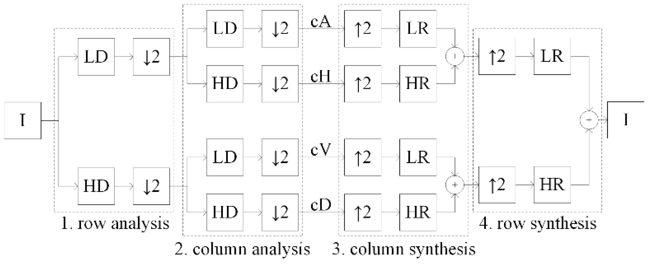
An image $I$, consisting of $X$ rows and $Y$ columns is represented as a function $I(x,y)$, where $0\le x\le X-1$ and $0\le y\le Y-1$ are the spatial coordinates of $I$. The pixel values are dependent on the kind of image (binary, grayscale, or color). In this paper, we focus primarily on grayscale and color images. Thus, the values of the pixels are referred to as $I(x,y)$ for grayscale images and as $I(x,y,z)$ for color images, where $z=1,2,3$—color number (red, green, and blue for example). DWT of image is implemented by sequentially using filter banks (wavelet filters). The scheme of a one-level two-dimensional DWT of images is shown in Figure 1.

• Row analysis is performed by decomposing the image along the rows with low-pass $LD$ and highpass $HD$ wavelet filters and downsampling $\downarrow 2$.
• Column analysis is performed by decomposing the coefficients obtained at stage 1, by columns similar to the row analysis.

We get four sets of coefficients $cA,cH,cV,cD$ of image decomposition, called approximating and detailing (horizontal, vertical, and diagonal), respectively, as a result of direct DWT of the original image $I$.

3.

Column synthesis is performed by upsampling $\uparrow 2$ the coefficients $cA,cH,cV,cD$, restoration with lowpass $HR$ and highpass $HR$ filters and summation of results.

4.

Row synthesis is performed for coefficients obtained at stage 3, by rows with the technique similar to the column synthesis.

The original image $I$ is restored as a result of the synthesis (inverse DWT) from the coefficients $cA,cH,cV,cD$. The original image should be completely restored. However, in practice, quantization noise occurs due to the digital format of the image representation.

We will assume that the wavelet filters $F$ consist of the coefficients $f_{F,i}$, where $i=0,\dots ,k-1$ is the coefficient number, where $k$ is the number of the filter coefficients. The next operation is called a convolution and is performed as follows:

$$I^{\prime }(x,y)={\displaystyle \sum _{i=0}^{k-1}I(x,y+i)\cdot f_{F,k-1-i}},I^{″}(x,y)={\displaystyle \sum _{i=0}^{k-1}I(x+i,y)\cdot f_{F,k-1-i}},$$

where $I^{\prime }$—result of row convolution, $I^{″}$—result of column convolution. We shall consider only wavelets with compact support. The coefficients of the wavelet filters are related by the equation [15]

$$f_{HD,i}={(-1)}^{i+1}{f}_{LD,k-1-i},f_{LR,i}=f_{LD,k-1-i},f_{HR,i}={(-1)}^i{f}_{LD,i}.$$

(1)

The question arises about the minimum bit-width of the wavelet filters coefficients, efficient from the point of view of hardware implementation on modern devices, and necessary to achieve a high image quality. The speed of operations with numbers in a fixed-point format is higher than in a floating-point format on modern devices, which can be used to develop real time image and video processing devices. Therefore, the coefficients of wavelet filters are quantized and converted into a format with a fixed-point in the proposed method as follows: scaled by $2^n$ and rounded up $\left(\lceil 2^n{f}_{F,i}\rceil \right)$. The bit-width $r$ of the filter coefficients can be determined by the formula $r=n+1$ in this case. The values of the pixels of the processed image should be normalized as follows: all the values obtained as a result of the image restoration are divided into $2^{4n}$ and rounded down $\left(\lfloor I(x,y)\rfloor \right)$.

Rounding up and rounding down are analogous to cutting the fractional part of the number with increasing the integer part by one in the case of rounding up. The rounding errors will have different signs and partially compensate each other when rounding is performed in different directions. The use of rounding operations in this order requires less resources for hardware implementation than rounding operations to the nearest. This is because the coefficients of the wavelet filters are known beforehand and their quantization with rounding up can be done previously. Thus, the coefficients of the wavelet filters will be used in the form of constants in the hardware part. The convolution is performed using arithmetic logic devices and its result is rounded down by cutting the fractional part that does not require additional hardware and time costs.

The error of the proposed method is estimated using the mean square error (MSE) of image, calculated for grayscale $(MS{E}_{grayscale})$ [28] and color $(MS{E}_{color})$ [29] images by the following formulas:

$$MS{E}_{grayscale}={\displaystyle \sum _{x=0}^{X-1}{\displaystyle \sum _{y=0}^{Y-1}\frac{{\left[I_1(x,y)-I_2(x,y)\right]}^2}{X\cdot Y}}},MS{E}_{color}=\frac{1}{3}{\displaystyle \sum _{z=1}^3{\displaystyle \sum _{x=0}^{X-1}{\displaystyle \sum _{y=0}^{Y-1}\frac{{\left[I_1(x,y,z)-I_2(x,y,z)\right]}^2}{X\cdot Y}}}}.$$

We used peak signal-to-noise ratio $(PSNR)$ between two images to quantify the image processing quality. This characteristic is measured in decibels (dB) and is calculated by the following formula [28]:

$$PSNR=10{\log }_{10}\left(\frac{M^2}{MSE}\right),$$

where $M$ is the maximum amplitude of the input image.

Theoretical analysis of the maximum error of DWT of images using the proposed method is presented in the next section.

3. Results

3.1. Theoretical Analysis of the Maximum Error of DWT of Images

The error arises initially when the filter coefficients are rounding up (quantization noise). Then, it increases with convolutions, upsampling and summing the results of convolution. We introduce the following notation. Rounding down after normalizing the values of the restored image also has an effect. Note the important facts:

• The absolute error of the DWT is maximal when all pixel values in the image are maximal.
• The analyzing and synthesizing wavelet filters consist of the same coefficients, according to formula (1), hence, the limited absolute errors of computations will also be equal. Therefore, within the framework of theoretical calculations, wavelet filters are classified only into lowpass $L$ and highpass $H$ ones.
• The sums of the lowpass and highpass wavelet filter coefficients are equal to $\sqrt{2}$ and $0$, respectively [15].

We introduce the following notation.

• $E_{j,F}$—limited absolute error (LAE) of calculating the value of the coefficient at the $j$-th stage, resulting from convolution with a sequence of wavelet filters $F$;
• $S_F$—the exact value of the sum of the coefficients of the wavelet filter $F$;
• $T_{j,F}$—the exact value of the calculations in the $j$-th stage, after convolution with a sequence of wavelet filters $F$.

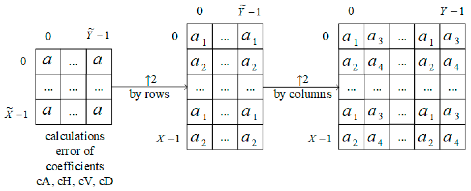
The errors for all the coefficients $cA,cH,cV,cD$ of image decomposition are separated into two groups (Figure 2, where $\tilde{X}=\frac{X+k}{2}-1$ and $\tilde{Y}=\frac{Y+k}{2}-1$) as a result of upsampling. Upsampling is applied twice during image recovery. We get four groups of errors as a result. Thus, to the introduced notations, it is necessary to add an additional index, which denotes calculations by the spatial characteristics of the coefficients.

We carry out theoretical calculations for an estimation of the maximum error of DWT of images:

Stage 1. Rounding up the filter coefficients. Calculate the exact values of the sums $S_F$ and $S_{F,l}$ of coefficients and errors $E_{1,F}$ and $E_{1,F,l}$ of rounding up the filters $L$ and $H$ coefficients, $l=1,2$:

$$S_L={\displaystyle \sum _{j=0}^{k-1}{2}^n{f}_{L,j}}=2^n{\displaystyle \sum _{j=0}^{k-1}{f}_{L,j}}=2^n\cdot \sqrt{2}=2^{n+\frac{1}{2}},S_H={\displaystyle \sum _{j=0}^{k-1}{2}^n{f}_{H,j}}=2^n{\displaystyle \sum _{j=0}^{k-1}{f}_{H,j}}=2^n\cdot 0=0,$$

$$S_{L,1}={\displaystyle \sum _{j=0}^{\frac{k}{2}-1}{2}^n{f}_{L,2j}},S_{L,2}={\displaystyle \sum _{j=0}^{\frac{k}{2}-1}{2}^n{f}_{L,2j+1}},S_{H,1}={\displaystyle \sum _{j=0}^{\frac{k}{2}-1}{2}^n{f}_{H,2j}},S_{H,2}={\displaystyle \sum _{j=0}^{\frac{k}{2}-1}{2}^n{f}_{H,2j+1}},$$

$$E_{1,L}={\displaystyle \sum _{j=0}^{k-1}\left(\lceil 2^n{f}_{L,j}\rceil -2^n{f}_{L,j}\right)},E_{1,H}={\displaystyle \sum _{j=0}^{k-1}\left(\lceil 2^n{f}_{H,j}\rceil -2^n{f}_{H,j}\right)},E_{1,L,1}={\displaystyle \sum _{j=0}^{\frac{k}{2}-1}\left(\lceil 2^n{f}_{L,2j}\rceil -2^n{f}_{L,2j}\right)},$$

$$E_{1,L,2}={\displaystyle \sum _{j=0}^{\frac{k}{2}-1}\left(\lceil 2^n{f}_{L,2j+1}\rceil -2^n{f}_{L,2j+1}\right)},E_{1,H,1}={\displaystyle \sum _{j=0}^{\frac{k}{2}-1}\left(\lceil 2^n{f}_{H,2j}\rceil -2^n{f}_{H,2j}\right)},E_{1,H,2}={\displaystyle \sum _{j=0}^{\frac{k}{2}-1}\left(\lceil 2^n{f}_{H,2j+1}\rceil -2^n{f}_{H,2j+1}\right)}.$$

Stage 2. Row decomposition. Calculate the exact values $T_{2,F}$ and errors $E_{2,F}$ of row decomposition with filters $L$ and $H$:

$$T_{2,L}=S_L\cdot M,E_{2,L}=E_{1,L}\cdot M,E_{2,H}=E_{1,H}\cdot M.$$

All the results of the convolution $T_{j,F}$ with the filter $H$ are zero.

Stage 3. Column decomposition. Calculate the exact values $T_{3,F}$ and errors $E_{3,F}$ of column decomposition with filters $L$ and $H$:

$$T_{3,LL}=T_{2,L}\cdot S_L,E_{3,LL}=(T_{2,L}+E_{2,L})(S_L+E_{1,L})-T_{3,LL},E_{3,LH}=(T_{2,L}+E_{2,L})E_{1,H},$$

$$E_{3,HL}=E_{2,H}(S_L+E_{1,L}),E_{3,HH}=E_{2,H}{E}_{1,H}.$$

Stage 4. Column reconstruction. Calculate the exact values $T_{4,F,l}$ and errors $E_{4,F,l}$ of column reconstruction with filters $L$ and $H$, $l=1,2$:

$$T_{4,LLL,l}=T_{3,LL}\cdot S_{L,l},E_{4,LLL,l}=(T_{3,LL}+E_{3,LL})(S_{L,l}+E_{1,L,l})-T_{4,LLL,l},E_{4,LHH,l}=E_{3,LH}(S_{H,l}+E_{1,H,l}),$$

$$E_{4,HLL,l}=E_{3,HL}(S_{L,l}+E_{1,L,l}),E_{4,HHH,l}=E_{3,HH}(S_{H,l}+E_{1,H,l}).$$

Stage 5. Column summation. Calculate the errors $E_{5,F,l}$ of sums $E_{4,F,l}$, $l=1,2:$

$$E_{5,L,l}=E_{4,LLL,l}+E_{4,LHH,l},E_{5,H,l}=E_{4,HLL,l}+E_{4,HHH,l}.$$

Stage 6. Row reconstruction. Calculate the exact values $T_{6,F,l}$ and errors $E_{6,f,l}$ of row reconstruction with filters $L$ and $H$, $l=1,2,3,4$:

$$T_{6,L,1}=T_{4,LLL,1}\cdot S_{L,1},T_{6,L,2}=T_{4,LLL,2}\cdot S_{L,1},T_{6,L,3}=T_{4,LLL,1}\cdot S_{L,2},T_{6,L,4}=T_{4,LLL,2}\cdot S_{L,2},$$

$$E_{6,L,1}=(T_{4,L,1}+E_{5,L,1})(S_{L,1}+E_{1,L,1})-T_{6,L,1},E_{6,L,2}=(T_{4,L,2}+E_{5,L,2})(S_{L,1}+E_{1,L,1})-T_{6,L,2},$$

$$E_{6,L,3}=(T_{4,L,1}+E_{5,L,1})(S_{L,2}+E_{1,L,2})-T_{6,L,3},E_{6,L,4}=(T_{4,L,2}+E_{5,L,2})(S_{L,2}+E_{1,L,2})-T_{6,L,4},$$

$$E_{6,H,1}=E_{5,H,1}(S_{L,1}+E_{1,H,1}),E_{6,H,2}=E_{5,H,2}(S_{L,1}+E_{1,H,1}),E_{6,H,3}=E_{5,H,1}(S_{L,2}+E_{1,H,2}),$$

$$E_{6,H,4}=E_{5,H,2}(S_{L,2}+E_{1,H,2}).$$

Stage 7. Row summation. Calculate the errors $E_{7,l}$ of sums $E_{6,F,l}$, $l=1,2,3,4$:

$$E_{7,l}=E_{6,L,l}+E_{6,H,l}.$$

Stage 8. Normalizing. Calculate the errors $E_{8,l}$ of division $E_{7,l}$ by $2^{4n}$, $l=1,2,3,4$:

$$E_{8,l}=\frac{E_{7,l}}{2^{4n}}.$$

Stage 9. Rounding down of pixel values. Calculate the errors $E_{9,l}$ of rounding down $E_{8,l}$, $l=1,2,3,4$:

$$E_{9,l}=\lfloor E_{8,l}\rfloor .$$

The obtained values $E_{9,l}$ $(l=1,2,3,4)$ represent the resulting error of the method and allow for the calculation of the PSNR.

$$PSNR=10{\log }_{10}\left(\frac{4M^2}{{\displaystyle \sum _{l=1}^4{E}_{9,l}^2}}\right),$$

(2)

where $\frac{1}{4}{\displaystyle \sum _{l=1}^4{E}_{9,l}^2}=MS{E}_{grayscale}=MS{E}_{color}$.

The results of the theoretical analysis can be applied to any wavelet with a compact support. Comparison of the results of calculations using formula (2) and simulation is presented below.

3.2. Simulation of the Image DWT

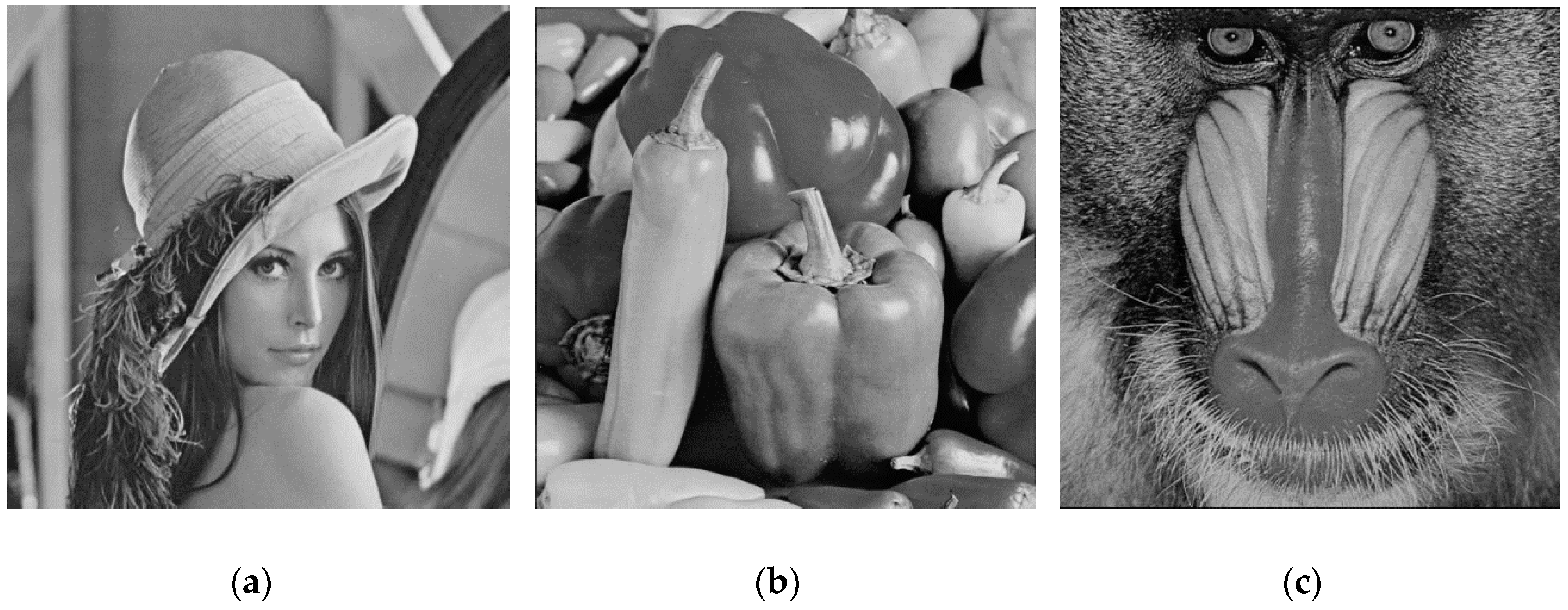
The simulation was carried out in the Matlab software version R2017b (40502181, ETU-LETI, St. Petersburg, Russia) of the 8-bit $(M=255)$ grayscale images “Lena” (Figure 3a) with low-frequency pattern, “Pepper” (Figure 3b) with low frequency pattern, and “Baboon” (Figure 3c) with a high-frequency pattern.

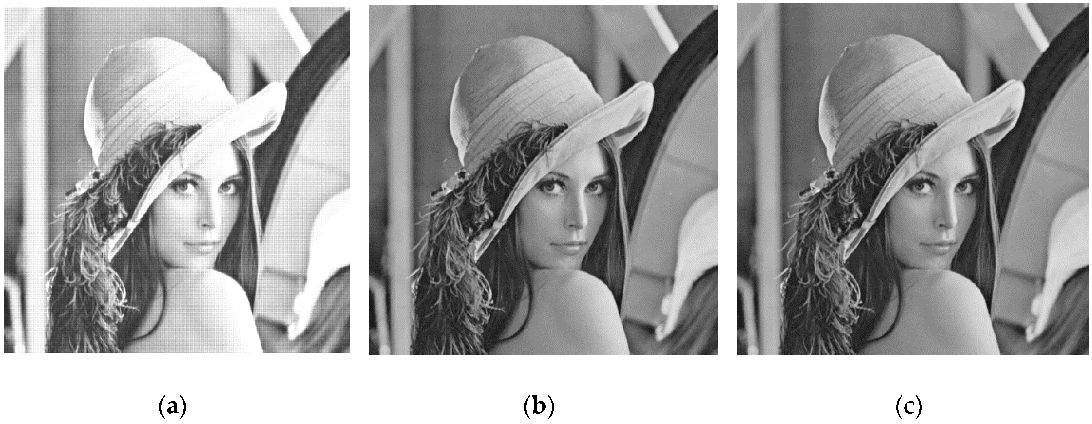
The Daubechies wavelets $db\frac{k}{2}$ $(k=4,8,12,\dots ,40)$, symlets $sym\frac{k}{2}$ $(k=4,8,12,\dots ,40)$, and coiflets $coif\frac{k}{6}$ $(k=6,12,\dots ,30)$ are used. Wavelet filters are obtained using the command “wfilters”. Decomposition and reconstruction of the image are carried out using the commands “dwt2” and “idwt2”, respectively. Simulation, as well as theoretical analysis, was carried out with quantized coefficients in accordance with the proposed implementation of the DWT of images. An example of the simulation results with image “Lena” and a wavelet $db4$ is shown in Figure 4.

Figure 4 shows that as the value of $n$ increases, the processing quality gradually improves: when $n=5$ image seem lightened; when $n=10$, the restored image is indistinguishable from the original image; when $n=12$, the restored image is identically equal to the original image.

The results of theoretical calculations of the maximum error of the DWT of images, obtained according to the Formula (2) for different values of $n$ $(n=8,\dots ,15)$, Daubechies wavelets $db\frac{k}{2}$ $(k=4,8,12,\dots ,40)$, and 8-bit image $(M=255)$, are presented in

Table 1. The results of theoretical calculations for Daubechies wavelets (PSNR, dB). PSNR—peak signal-to-noise ratio.

$\mathit{n}$	$\mathit{d}\mathit{b}\mathbf{2}$	$\mathit{d}\mathit{b}\mathbf{4}$	$\mathit{d}\mathit{b}\mathbf{6}$	$\mathit{d}\mathit{b}\mathbf{8}$	$\mathit{d}\mathit{b}\mathbf{10}$	$\mathit{d}\mathit{b}\mathbf{12}$	$\mathit{d}\mathit{b}\mathbf{14}$	$\mathit{d}\mathit{b}\mathbf{16}$	$\mathit{d}\mathit{b}\mathbf{18}$	$\mathit{d}\mathit{b}\mathbf{20}$
8	33.43	26.70	22.95	22.52	20.03	16.63	16.43	13.39	14.20	10.97
9	40.17	33.43	28.32	28.10	25.62	22.46	22.83	19.97	19.32	18.34
10	46.37	38.35	35.58	34.86	30.99	29.56	28.42	26.28	25.79	25.62
11	54.15	46.37	41.85	41.85	38.71	37.72	34.02	33.43	32.06	31.57
12	$\infty$	54.15	54.15	46.37	46.37	41.85	41.85	41.60	38.71	37.72
13	$\infty$	$\infty$	$\infty$	54.15	54.15	49.38	54.15	49.38	46.37	46.37
14	$\infty$	$\infty$	$\infty$	$\infty$	$\infty$	$\infty$	$\infty$	$\infty$	54.15	54.15
15	$\infty$	$\infty$	$\infty$	$\infty$	$\infty$	$\infty$	$\infty$	$\infty$	$\infty$	$\infty$

.

One can see from Table 1, that as the number of wavelet filters coefficients increases, their absolute values decrease. This leads to an increase in the error of their rounding and the resulting error of the DWT. Therefore, it is necessary to increase the value of $n$ to maintain the same level of calculation accuracy.

The results of simulation of the DWT of the 8-bit $(M=255)$ grayscale image “Lena” for different values of $n$ $(n=8,\dots ,15)$ and Daubechies wavelets $db\frac{k}{2}$ $(k=4,8,12,\dots ,40)$ are presented in

Table 2. The results of simulation of “Lena” with Daubechies wavelets (PSNR, dB).

$\mathit{n}$	$\mathit{d}\mathit{b}\mathbf{2}$	$\mathit{d}\mathit{b}\mathbf{4}$	$\mathit{d}\mathit{b}\mathbf{6}$	$\mathit{d}\mathit{b}\mathbf{8}$	$\mathit{d}\mathit{b}\mathbf{10}$	$\mathit{d}\mathit{b}\mathbf{12}$	$\mathit{d}\mathit{b}\mathbf{14}$	$\mathit{d}\mathit{b}\mathbf{16}$	$\mathit{d}\mathit{b}\mathbf{18}$	$\mathit{d}\mathit{b}\mathbf{20}$
8	39.54	32.82	29.00	28.59	25.97	22.55	22.41	19.29	20.21	16.94
9	47.00	39.59	34.29	34.01	31.61	28.42	28.92	25.90	25.33	24.35
10	$\infty$	44.99	42.60	40.95	37.51	35.72	34.89	32.48	31.88	31.78
11	$\infty$	53.40	50.53	48.63	46.00	44.42	40.59	39.78	38.76	38.09
12	$\infty$	$\infty$	$\infty$	$\infty$	51.75	50.72	49.55	48.04	46.32	44.36
13	$\infty$	$\infty$	$\infty$	$\infty$	$\infty$	$\infty$	$\infty$	$\infty$	$\infty$	$\infty$
14	$\infty$	$\infty$	$\infty$	$\infty$	$\infty$	$\infty$	$\infty$	$\infty$	$\infty$	$\infty$
15	$\infty$	$\infty$	$\infty$	$\infty$	$\infty$	$\infty$	$\infty$	$\infty$	$\infty$	$\infty$

.

The values of each cell from Table 2 are not lesser than the values of the corresponding cell from Table 1. This difference is explained by the fact that in theoretical calculations, we are trying to predict the worst case. Thus, the results of simulation of the DWT of images confirm the results of theoretical calculations.

Let us compile

Table 3. The values $n$ at which the result of discrete wavelet transform (DWT) of images “Lena”, “Pepper”, and “Baboon” with a Daubechies wavelets reaches quality of $PSNR=40$ dB and $PSNR=\infty$.

$\mathit{P}\mathit{S}\mathit{N}\mathit{R}$	Results	$\mathit{d}\mathit{b}\mathbf{2}$	$\mathit{d}\mathit{b}\mathbf{4}$	$\mathit{d}\mathit{b}\mathbf{6}$	$\mathit{d}\mathit{b}\mathbf{8}$	$\mathit{d}\mathit{b}\mathbf{10}$	$\mathit{d}\mathit{b}\mathbf{12}$	$\mathit{d}\mathit{b}\mathbf{14}$	$\mathit{d}\mathit{b}\mathbf{16}$	$\mathit{d}\mathit{b}\mathbf{18}$	$\mathit{d}\mathit{b}\mathbf{20}$
40	Theoretical	9	11	11	11	12	12	12	12	13	13
	Simulation (“Lena”)	9	10	10	10	11	11	11	12	12	12
	Simulation (“Pepper”)	9	10	10	10	11	11	11	11	12	12
	Simulation (“Baboon”)	8	9	10	10	11	11	11	11	11	12
$\infty$	Theoretical	12	13	13	14	14	14	14	14	15	15
	Simulation (“Lena”)	10	12	12	12	13	13	13	13	13	14
	Simulation (“Pepper”)	10	12	12	12	13	13	13	13	13	14
	Simulation (“Baboon”)	10	11	12	12	12	13	13	13	13	13

,

Table 4. The values $n$ at which the result of DWT of images “Lena”, “Pepper”, and “Baboon” with a symlets reaches the quality of $PSNR=40$ dB and $PSNR=\infty$.

$\mathit{P}\mathit{S}\mathit{N}\mathit{R}$	Results	$\mathit{s}\mathit{y}\mathit{m}\mathbf{2}$	$\mathit{s}\mathit{y}\mathit{m}\mathbf{4}$	$\mathit{s}\mathit{y}\mathit{m}\mathbf{6}$	$\mathit{s}\mathit{y}\mathit{m}\mathbf{8}$	$\mathit{s}\mathit{y}\mathit{m}\mathbf{10}$	$\mathit{s}\mathit{y}\mathit{m}\mathbf{12}$	$\mathit{s}\mathit{y}\mathit{m}\mathbf{14}$	$\mathit{s}\mathit{y}\mathit{m}\mathbf{16}$	$\mathit{s}\mathit{y}\mathit{m}\mathbf{18}$	$\mathit{s}\mathit{y}\mathit{m}\mathbf{20}$
40	Theoretical	9	11	11	11	12	12	12	12	12	13
	Simulation (“Lena”)	9	10	10	10	11	11	11	11	12	12
	Simulation (“Pepper”)	9	10	10	10	11	11	11	11	12	12
	Simulation (“Baboon”)	8	9	10	10	11	11	11	11	12	12
$\infty$	Theoretical	12	13	13	14	14	14	14	14	15	15
	Simulation (“Lena”)	10	12	12	12	13	13	13	13	13	13
	Simulation (“Pepper”)	10	12	12	12	13	13	13	13	13	13
	Simulation (“Baboon”)	10	11	12	12	12	13	13	13	13	13

and

Table 5. The values $n$ at which the result of DWT of images “Lena”, “Pepper” and “Baboon” with a coiflets reaches quality of $PSNR=40$ dB and $PSNR=\infty$.

$\mathit{P}\mathit{S}\mathit{N}\mathit{R}$	Results	$\mathit{c}\mathit{o}\mathit{i}\mathit{f}\mathbf{1}$	$\mathit{c}\mathit{o}\mathit{i}\mathit{f}\mathbf{2}$	$\mathit{c}\mathit{o}\mathit{i}\mathit{f}\mathbf{3}$	$\mathit{c}\mathit{o}\mathit{i}\mathit{f}\mathbf{4}$	$\mathit{c}\mathit{o}\mathit{i}\mathit{f}\mathbf{5}$
40	Theoretical	10	11	11	12	12
	Simulation (“Lena”)	9	11	11	11	11
	Simulation (“Pepper”)	9	10	11	11	11
	Simulation (“Baboon”)	9	10	10	11	11
$\infty$	Theoretical	13	13	14	14	14
	Simulation (“Lena”)	12	12	12	13	13
	Simulation ("Pepper")	12	12	12	13	13
	Simulation ("Baboon")	11	12	12	13	13

as follows: we note the values of $n$, for which, according to theoretical calculation and simulation results, the 8-bit $(M=255)$ grayscale images “Lena”, “Pepper”, and “Baboon”, processed with the Daubechies wavelets $db\frac{k}{2}$ $(k=4,8,12,\dots ,40)$, symlets $sym\frac{k}{2}$ $(k=4,8,12,\dots ,40)$, and coiflets $coif\frac{k}{6}$ $(k=6,12,\dots ,30)$, reach a high $(PSNR\ge 40)$ and maximum $(PSNR=\infty )$ quality. For example, for a wavelet $db2$, a high quality of 40 dB is achieved at $n=9$ (40.17 dB according to Table 1) and at $n=9$ (47.00 dB according to Table 2); the maximum quality is achieved when $n=12$ (according to Table 1) and when $n=10$ (according to Table 2). The remaining columns are filled in the same way.

4. Discussion

We can make the following conclusions, based on the results of theoretical calculations and simulation, partially presented in Table 1, Table 2, Table 3, Table 4 and Table 5.

• All values of the PSNR obtained as a result of the theoretical calculations are not lesser than the values of the PSNR obtained as a result of the simulation, as in theoretical calculations, we are trying to predict the worst case.
• The result of image processing “Baboon” with a high-frequency pattern is slightly superior in quality to the result of images processing “Lena” and “Pepper” with low-frequency patterns for each value of $n$ for all wavelets used. Thus, the higher the frequency of the image pattern, the less the effect of quantization noise.
• Similar results were obtained using various types of wavelets. Thus, the number $k$ of the wavelet filter coefficients is the only important factor that affects the values of $n$ and bit-width $r$ of the wavelet filter coefficients that is necessary for high-quality image processing.
• The minimum values of $n$ and bit-width $r$ at which the result of a DWT of images does not contain distortions visible to the viewer $(PSNR\ge 40)$ can be determined by the formula

  $$n\ge 10+\lfloor \sqrt{\frac{k}{4}}\rfloor ,r=n+1\ge 11+\lfloor \sqrt{\frac{k}{4}}\rfloor .$$

  (3)
• The minimum values of $n$ and bit-width $r$ at which the result of a DWT of images does not contain $(PSNR=\infty )$ can be determined by the formula

  $$n\ge 12+\lfloor \sqrt{\frac{k}{4}}\rfloor ,r=n+1\ge 13+\lfloor \sqrt{\frac{k}{4}}\rfloor .$$

  (4)

Formulas (3) and (4) are approximate. The values obtained at their use are sometimes redundant, that is, they exceed the digits presented in Table 3, Table 4 and Table 5.

The developed approach to the determination of the bit-width $r$ of wavelet filter coefficients can be used to reduce the hardware and time costs for the practical implementation of a system that performs DWT of image. For example, in the literature [23], it is indicated that the representation of the wavelet filter coefficients in the format of real numbers requires at least 32 bits. Further, the authors of this paper prove the possibility of reducing this bit-width to 16 bits by converting the wavelet filter coefficients to the format of a fixed-point number. At the same time, in the literature [23], it is said about the possibility of further decreasing the bit-width of the wavelet filter coefficients with the risk of errors due to the overflow of the range of the computer system. Our theoretical and practical analysis proves the possibility of reducing such a bit-width to 12–15 bits without the risk of errors, depending on the type of wavelet used, which is 6–25% less compared with the results of the work of [23].

In the work of [24,25], the authors consider hardware implementations of systems implementing DWT of signals with filters, the coefficients of which are quantized by 5 and 16 bits each. As noted above, 16 bits is an excessive bit-width when processing images. At the same time, we have shown that using only 5 bits will not allow us to obtain acceptable image processing quality.

The hardware implementation of our method has the following advantages.

• Calculations are performed on fixed-point numbers faster than on floating-point numbers.
• The operations of multiplying and dividing by $2^n$ in a two complement correspond to a comma shift to $n$ digits to the right or to the left, respectively, which simplifies and speeds up their execution.
• Rounding up and rounding down are analogous to cutting the fractional part of the number with increasing the integer part by one, in the case of rounding up. This avoids the difficulties associated with determining the digits of the fractional part of the rounded numbers.
• The resources used in the hardware implementation can be reduced when using a specific wavelet, as the highest bits of the filters coefficients are zero.

5. Conclusions

This paper gives a contribution to solving the problem of choosing the efficient bit-width for the coefficients of discrete wavelet transform (DWP) filter banks for image processing. The method was developed for estimating maximum error of image processing that can arise as a result of DWT of images by the Formula (2). The derived Formulas (3) and (4) allow determining the minimum bit-width of filter banks coefficients, at which the result of DWT achieves high quality or the processed image does not differ from the original one, depending on the wavelet type used. All calculations are performed only in fixed-point numbers and the rounding operations are simplified.

The obtained results open the possibility for efficient hardware implementation of the DWT of images on modern devices (FPGA, ASIC, etc.) for denoising and image processing in various areas, such as medical image processing, biology, physics, and astronomy, as well as in industrial, defense, and law enforcement fields and other fields of science and technology.

References

- Noor, S.S.M.; Michael, K.; Marshall, S.; Ren, J. Hyperspectral Image Enhancement and Mixture Deep-Learning Classification of Corneal Epithelium Injuries. Sensors 2017, 17, 2644. [Google Scholar] [CrossRef] [PubMed]
- Ruszczycki, B.; Bernas, T. Quality of biological images, reconstructed using localization microscopy data. Bioinformatics 2018, 34, 845–852. [Google Scholar] [CrossRef] [PubMed]
- Li, H.; Kingston, A.; Myers, G.; Recur, B.; Sheppard, A. 3D X-Ray Source Deblurring in High Cone-Angle Micro-CT. IEEE Trans. Nucl. Sci. 2015, 62, 2075–2084. [Google Scholar] [CrossRef]
- Bianco, V.; Memmolo, P.; Paturzo, M.; Ferraro, P. On-speckle suppression in IR Digital Holography. Opt. Lett. 2016, 41, 5226–5229. [Google Scholar] [CrossRef] [PubMed]
- Kremer, J.; Stensbo-Smidt, K.; Gieseke, F.; Pedersen, K.S.; Igel, C. Big Universe, Big Data: Machine Learning and Image Analysis for Astronomy. IEEE Intell. Syst. 2017, 32, 16–22. [Google Scholar] [CrossRef] [Green Version]
- Torabi, M.; Mousavi, S.G.M.; Younesian, D. A High Accuracy Imaging and Measurement System for Wheel Diameter Inspection of Railroad Vehicles. IEEE Trans. Ind. Electron. 2018, 65, 8239–8249. [Google Scholar] [CrossRef]
- Peng, C.; Gao, X.; Wang, N.; Li, J. Superpixel-Based Face Sketch–Photo Synthesis. IEEE Trans. Circuits Syst. Video Technol. 2017, 27, 288–299. [Google Scholar] [CrossRef]
- Buades, A.; Coll, B.; Morel, J. A non-local algorithm for image denoising. IEEE Comput. Soc. Conf. Comput. Vis. Pattern Recognit. 2005, 2, 60–65. [Google Scholar]
- Varghese, J.; Subash, S.; Tairan, N. Fourier transform-based windowed adaptive switching minimum filter for reducing periodic noise from digital images. IET Image Process. 2016, 10, 646–656. [Google Scholar] [CrossRef]
- Vetterli, M.; Kovacevic, J.; Goyal, V.K. Foundations of Signal Processing; Cambridge University Press: Cambridge, UK, 2014; 715p. [Google Scholar]
- Daubechies, I. Ten Lectures on Wavelets; Society for Industrial and Applied Mathematics: Philadelphia, PA, USA, 1992; 380p. [Google Scholar]
- Mallat, S. A Wavelet Tour of Signal Process the Sparse Way, 3rd ed.; Academic Press: Cambridge, MA, USA, 2009; 824p. [Google Scholar]
- Damasevicius, R.; Ziberkas, G. Energy Consumption and Quality of Approximate Image Transformation. Electron. Electr. Eng. 2012, 120. [Google Scholar] [CrossRef]
- Tan, L.; Jiang, J. Digital Signal Processing: Fundamentals and Applications, 2nd ed.; Academic Press: Cambridge, MA, USA, 2013; 876p. [Google Scholar]
- Bailey, G. Design for Embedded Image Processing on FPGAs; Wiley-IEEE Press: Hoboken, NJ, USA, 2011; 482p. [Google Scholar]
- Katkovnik, V.; Ponomarenko, M.; Egiazarian, K. Sparse approximations in complex domain based on BM3D modelling. Signal Process. 2017, 141, 96–108. [Google Scholar] [CrossRef]
- Katkovnik, V.; Egiazarian, K. Sparse phase imaging based on complex domain nonlocal BM3D techniques. Digit. Signal Process. 2017, 63, 72–85. [Google Scholar] [CrossRef]
- Liu, Y.; Lai, E.M.-K. Design and implementation of an RNS-based 2-D DWT processor. IEEE Trans. Consumer Electr. 2004, 50, 376–385. [Google Scholar] [CrossRef]
- Cheng, C.-C.; Huang, C.-T.; Chen, C.-Y.; Lian, C.-J.; Chen, L.-G. On-Chip Memory Optimization Scheme for VLSI Implementation of Line-Based Two-Dimentional Discrete Wavelet Transform. IEEE Trans. Circuits Syst. Video Technol. 2007, 17, 814–822. [Google Scholar] [CrossRef] [Green Version]
- Meher, P.K.; Mohanty, B.K.; Patra, J.C. Hardware-Efficient Systolic-Like Modular Design for Two-Dimensional Discrete Wavelet Transform. IEEE Trans. Circuits Syst. II Exp. Briefs 2008, 55, 151–155. [Google Scholar] [CrossRef] [Green Version]
- Laan, W.J.; Jalba, A.C.; Roerdink, J.B.T.M. Accelerating Wavelet Lifting on Graphics Hardware Using CUDA. IEEE Trans. Parallel Distrib. Syst. 2011, 22, 132–146. [Google Scholar] [CrossRef] [Green Version]
- Safari, A.; Niras, C.V.; Kong, Y. Power-performance enhancement of two-dimensional RNS-based DWT image processor using static voltage scaling. Integr. VLSI J. 2016, 53, 145–156. [Google Scholar] [CrossRef]
- Adams, M.D.; Kossentni, F. Reversible integer-to-integer wavelet transforms for image compression: performance evaluation and analysis. IEEE Trans. Image 2000, 9, 1010–1024. [Google Scholar] [CrossRef] [PubMed] [Green Version]
- Chehaitly, M.; Tabaa, M.; Monteiro, F.; Dandache, A. A fast and configurable architecture for Discrete Wavelet Packet Transform. In Proceedings of the 2015 Conference on Design of Circuits and Integrated Systems (DCIS), Estoril, Portugal, 25–27 November 2015; pp. 1–6. [Google Scholar]
- Chehaitly, M.; Tabaa, M.; Monteiro, F.; Dandache, A. A ultr a high speed and configurable Inverse Discrete Wavelet Packet Transform architecture. In Proceedings of the 29th International Conference on Microelectronics, Beirut, Lebanon, 10–13 December 2017; pp. 1–4. [Google Scholar]
- Schlichthärle, D. Digital Filters: Basics and Design, 2nd ed.; Springer Science & Business Media: Berlin/Heidelberg, Germany 2011; 527p. [Google Scholar]
- Mehrnia, A.; Willson, A.N. A Lower Bound for the Hardware Complexity of FIR Filters. IEEE Circuits Syst. Mag. 2017, 18, 10–28. [Google Scholar] [CrossRef]
- Rao, K.R.; Yip, P.C. The Transform and Data Compression Handbook; CRC Press: Boca Raton, FL, USA, 2001; 399p. [Google Scholar]
- Basso, A.; Cavagnino, D.; Pomponui, V.; Vernone, A. Blind watermarking of color images using Karhunen–Loève transform keying. Comput. J. 2011, 54, 1076–1090. [Google Scholar] [CrossRef]
Figure 1.
The scheme of image DWT.
Figure 2.
The scheme of separation of errors with upsampling.
Figure 3.
Images used for simulation: (a) “Lena”; (b) “Pepper”; and (c) “Baboon”.
Figure 4.
The result of simulation of image “Lena” with a wavelet : (a) , dB; (b) , dB; and (c) , . PSNR—peak signal-to-noise ratio.