VSG Stability and Coordination Enhancement under Emergency Condition


1
Department of Electrical Engineering, North China Electric Power University, Baoding 071003, China
2
Goldwind Science and Technology, Co. Ltd., Beijing 100176, China
3
Electrical Engineering and Power Electronics Department, Vrije Universiteit Brussel, 1050 Brussels, Belgium
4
Department of Electronics System Engineering, Hanyang University, Ansan 15588, Korea, [email protected]
*
Author to whom correspondence should be addressed.
Electronics 2018, 7(9), 202; https://doi.org/10.3390/electronics7090202
Submission received: 17 August 2018
/
Revised: 11 September 2018
/
Accepted: 14 September 2018
/
Published: 17 September 2018
(This article belongs to the Special Issue Power Quality in Smart Grids)
Abstract
:Renewable energy sources are integrated into a grid via inverters. Due to the absence of an inherent droop in an inverter, an artificial droop and inertia control is designed to let the grid-connected inverters mimic the operation of synchronous generators and such inverters are called virtual synchronous generators (VSG). Sudden addition, removal of load or faults in the grid causes power and frequency oscillations in the grid. The steady state droop control of VSG is not effective in dampening such oscillations. Therefore, a new control scheme, namely bouncy control, has been introduced. This control uses a variable emergency gain, to enhance or reduce the power contribution of individual VSGs during a disturbance. The maximum power contribution of an individual VSG is limited by its power rating. It has been observed that this control, successfully minimized the oscillation of electric parameters and the power system approached steady state quickly. Therefore, by implementing bouncy control, VSGs can work in coordination to make the grid more robust. The proposed controller is verified through Lyapunov stability analysis.
1. Introduction
With the increases in the growth of renewable energy sources (RES)-based distributed generators (DG), the parallel connection of DG sources to form a microgrid has emerged as a commercially and technically feasible solution. A microgrid usually comprises of multiple DGs of different types, such as renewable energy sources (RES), non-renewable energy source and energy storage system (ESS). RES are dependent on the environmental condition and are usually uncontrollable (or offer marginal control), and therefore the presence of controllable sources is necessary for the steady operation of a microgrid. A centralized control called an energy management system (EMS) controls all the parallel operating DGs in microgrid; based on the electrical parameters of grid. EMS can be operated in a grid-connected microgrid as well as in an island-mode microgrid.
There are two main types of microgrid control: (i) control via communication, a centralized control that has comparatively a slower response (e.g., secondary or tertiary control); and (ii) control not requiring communication, a decentralized control that offers faster response toward any change in active and reactive power of a microgrid (e.g., primary control). [1,2,3,4]. The hierarchical control structure to normalize the operation of an islanded alternating current (AC) microgrid experiencing communication link failures is presented in [5]. In a microgrid, a droop control is normally used as a primary control due of its decentralized nature. It provides a firm coordination between multiple DGs operating in parallel. Different types of droop control are discussed in literature e.g., P-ω, P-V, Q-V, etc. [6,7,8,9].A drawback of droop control is a lack of inertia. In a conventional power system, a main source of electricity is a synchronous generator (SG), which has an inherent droop and inertia control that helps to synchronize multiple synchronous generators and share a real and reactive power equally among them. Moreover, because of its inherent inertia, it brings a system back to its steady state quickly after any disturbance.
The control of inverter which resembles the characteristics of synchronous generator, in terms of real and reactive power sharing ability and droop-control, was first proposed in [10], and was further developed for parallel inverters in [7]. The virtual synchronous generator (VSG) was first proposed in [11], because of its capability to stabilize using virtual rotational inertia; along with a droop control. The inverter control strategies that mimic synchronous generator have been presented as virtual synchronous generator [12], followed by virtual synchronous machines (VSM) in [13], virtual synchronous machine (VISMA) in [14], and synchronverter in [15].
However, VSG still has some weaknesses compared to synchronous generator due to its inappropriate sharing of active and reactive transient power (unsuitable coordination) and the lack of overload capability to ride through large oscillations that can cause severe oscillation problem at the time of disturbance in a microgrid [16]. A VSG control technique based on Hamilton approach is introduced to enhance the robustness of a system in [17].The alternate moment of inertia is a technique that uses different inertia coefficient to increase the damping of a system during oscillation [18], the smaller inertia is used to enhance the dynamic response of an inverter [19], the proper increase in damping ratio by observing the derivative of power, reactive power, voltage and the phase difference to solve the output power oscillation presented in [20], the power oscillation is damped by using a virtual stator reactance in [16], and sharing transient load by using the generator emulation method presented in [21] are a few techniques to address this issue.
• Microgrid isolation
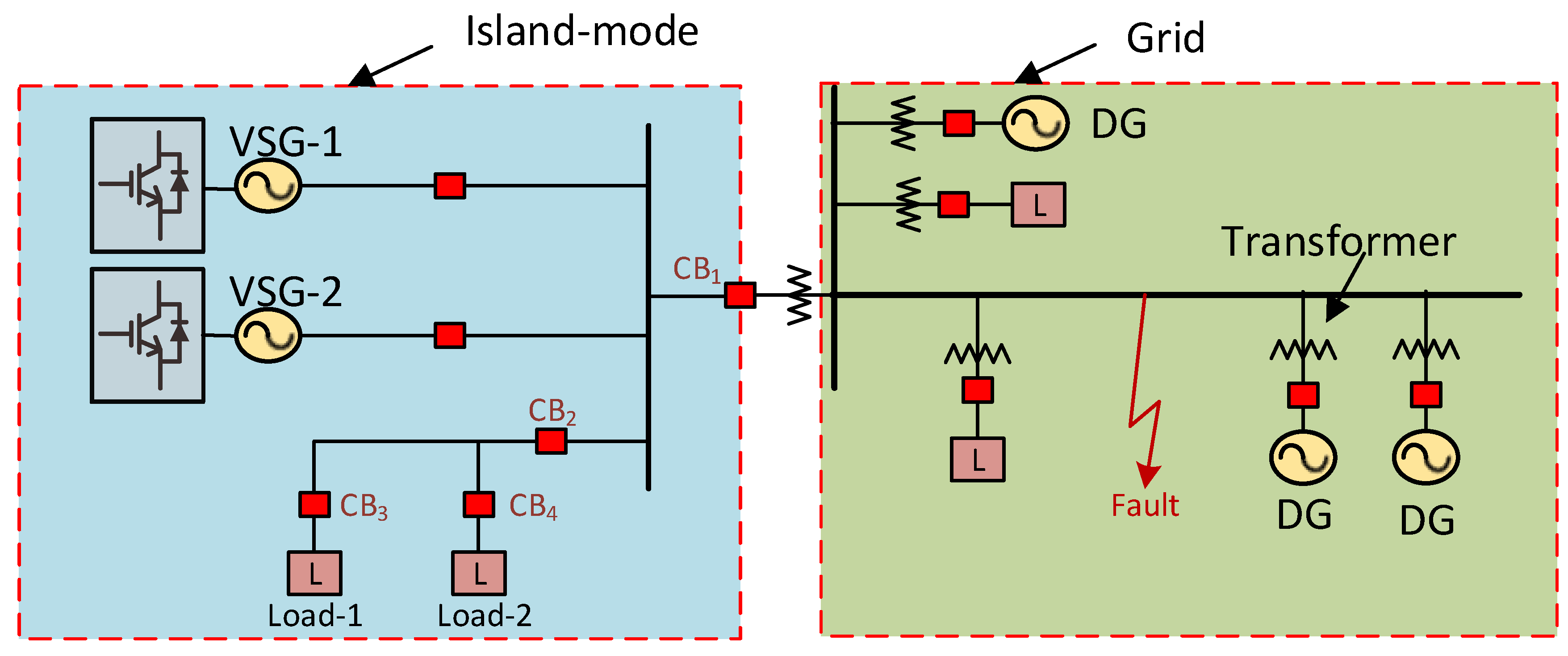
A microgrid is designed to operate in two basic modes: (i) island mode, and (ii) grid-connected mode. The transition to an island-mode or isolated microgrid can take place suddenly i.e., unscheduled or according to a schedule. In the scheduled transition, the main grid controller give a signal to a microgrid. This type of transition is relatively safe because of prior information of a disturbance. When a fault appears at the grid; that goes beyond the protection limits of a microgrid, then a microgrid opens the circuit breaker (CB) ‘1’ in Figure 1 to isolate itself from the main fault zone in a grid. It is an unscheduled type of transition (from grid-connected to island mode) and it can cause severe disturbance. The proper protection and control measures are needed to safeguard a power system under such disturbances.
Microgrids are designed to operate in island mode under the standards defined in IEEE-1547.4. The local loads within an island mode microgrid operate from the distributed generators DGs. These DGs can be RES, fuel generators, and energy storage batteries. The standards in IEEE-1547.4 suggest that a microgrid should be able to support its local loads, when any contingency happens at a main grid or it should have a proper plan of load-shedding; in terms of critical or non-critical load, when microgrid generation is not sufficient to support its local loads. An island microgrid is usually sensitive toward any change because it does not have grid support to counter any disturbance. Therefore, the change in load or any similar operation that causes transient behavior in an island-microgrid must be keenly observed and countermeasures must be taken to alleviate disturbance.
At the time of loading, unloading, or a fault, the oscillation in power and frequency of VSG arises that may lead to instability of an overall system or even termination in a worst case situation. The stabilization of VSG is evaluated on the basis of its ability to eliminate oscillations from the microgrid. The oscillation improvement by considering the droop coefficient has been done by our research group in [22]. The angular frequency of VSG is considered for varying J and D in previous research. VSG utilizes a phase locked loop (PLL) technique to obtain frequency and phase of grid for the sake of synchronization [23].
In this research, a new parameter ‘emergency gain’ is introduced to dampen the oscillation of VSG during an emergency condition. The equation is derived to show the dependency of a parameter on a derivative of angular frequency. The final swing equation for the additional parameter is also presented. A ‘bouncy control algorithm’ is designed to define the variable values of emergency gain; it enhances the stability of a microgrid. It basically improves the transient time by varying the dependence of change in power on the VSG. The control is designed, such that and (derivative of change in power) are influencing the sensitivity of VSG power during the recovery. Lyapunov stability analysis is implemented to show the effectiveness of the scheme [18,24,25]. The energy function of synchronous generator is built within a simulation to investigate the disturbance in a system. This technique can be also be implemented to improve the coordination of VSGs that are operating as a source or a load in an island microgrid; developed in [26,27].
2. Basic Operation of Virtual Synchronous Generator (VSG)
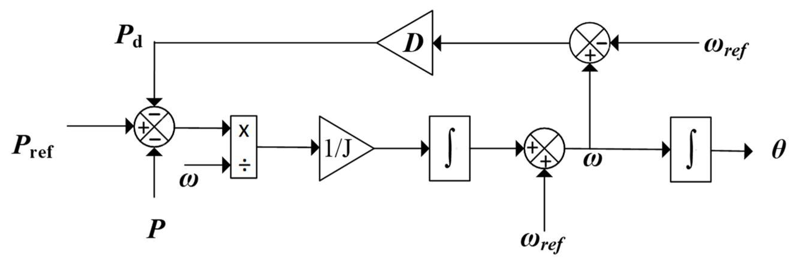
The block diagram of VSG control is shown in Figure 2. The control is designed in the dq-axis. The reference rotational frequency of the dq-axis is ‘’ in an isolated system, while in a grid-connected VSG, it adopts the rotational frequency of the grid. The double voltage current controller is used in this VSG control system. The basic second order swing equation for VSG control is shown in Equation (1). It has two parts: (i) a mechanical part, which controls the rotor motion by using control, and (ii) an electrical part, which control the stator voltage by using control.
where is the reference power provided by the governor, is the measured output power, D is the droop coefficient, J is the virtual inertia, ω is the virtual angular frequency of VSG, and is the angular frequency of the grid or power common coupling (PCC). is the maximum instantaneous power by VSG source. ‘’ is the excitation electromotive force and ‘’ is the stator current. ‘’ and ‘’ are a resistance and a reactance of stator winding in synchronous generator.
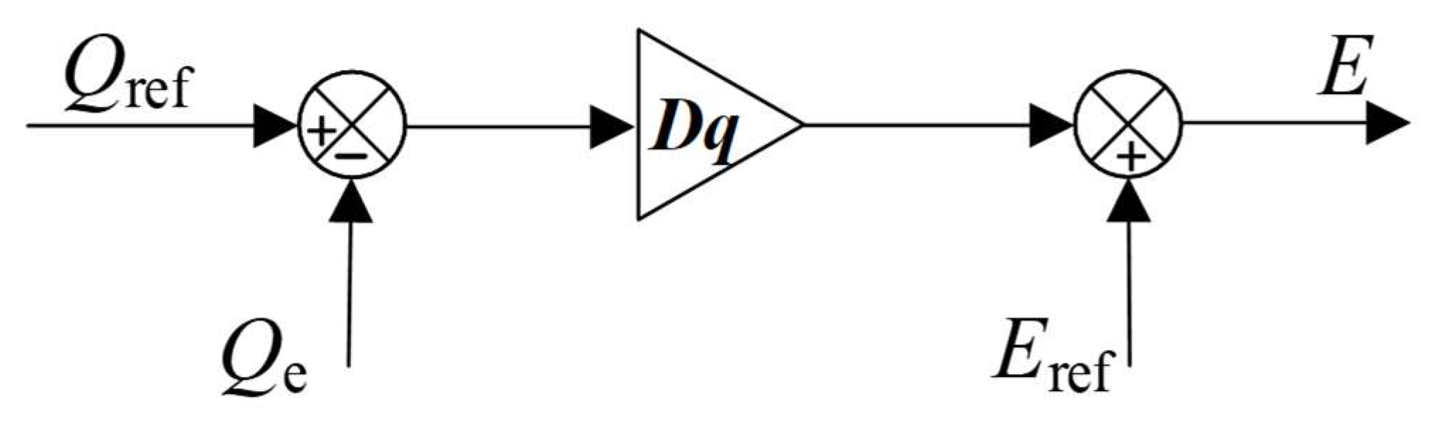
Equation (2) shows the basic active power and angular frequency (), and reactive power and voltage () droop control equations.
3. Emergency Power Control Scheme
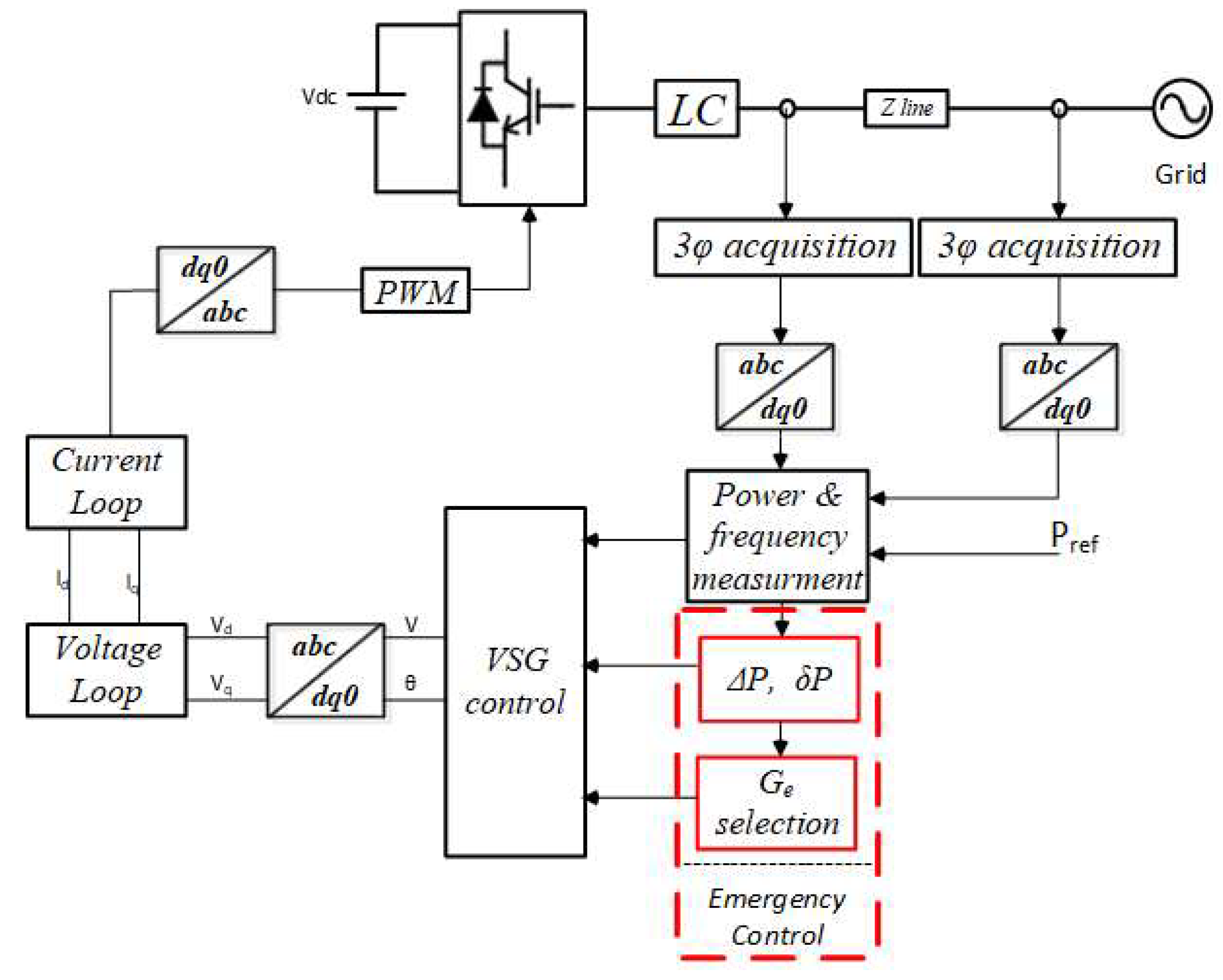
The VSG system is designed in the dq-axis, while considering the angular frequency of the grid and the dq-axis are same. The intention of using the dq-axis is to separate the effects of active and reactive power. The 3-Ф voltages and currents are first measured in abc-axis. After converting them into dq-axis, power and frequency are measured. The change in power and frequency is detected for the selection of & . VSG gives and at its output, which in turns generate pulse width modulation (PWM) after passing through voltage and current loop control. The overall control of grid connected VSG is displayed in Figure 4.
The coordination of multiple sources in a microgrid is a critical issue because of different power rating, inertia and droop ratio. The response of different sources is not the same, for example; the response of a synchronous generator is much slower than that of a VSG-based inverter controller. In the same way, the dynamic response of two VSG controllers connected in parallel is not identical; mainly because of droop and inertia, and therefore it is necessary to limit the response of a speedier source that approaches to its rated power sooner. This strategy has an ability to provide a protection to a swiftly responding source, whereas force other sources to response faster to bring equilibrium to the system.
The emergency power controller is designed such that the recovery time speeds up or slows down to stabilize a microgrid. The change in power during transition time along with the VSG control parameters decide the response of a VSG, which in turn define the stability of a system. In any control of a power system, the electric parameters strive to maintain their stable point during normal operation and return to a stable state after any disturbance. In the view of above consideration, the input parameters of VSG i.e. the change in active power ‘ΔP’ and the derivative of the active power ‘’ (equal to ), is used to stabilize a microgrid; without altering the control parameters (e.g., inertia and droop coefficient) of the VSG control.
The active power tries to approach its stable point after any disturbance. In VSG control, droop coefficient usually defines the static stability, whereas the dynamic stability is dependent on both droop coefficient and inertia. Hence, P-ω droop control defines the new stable point of VSG electric parameters, such as power and angular frequency. The angular frequency is considered as a measure of the stability of the VSG, and therefore, to improve the stability of a VSG or a microgrid, the angular frequency stability needs to be enhanced.
3.1. Bouncy Control
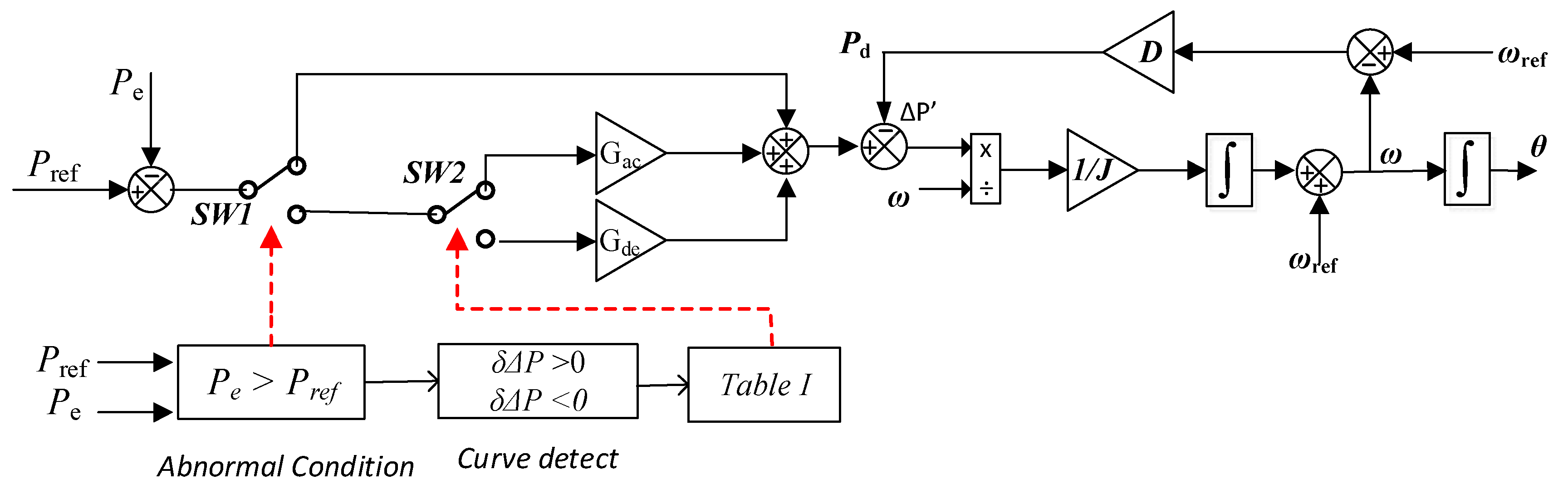
A bouncy control is designed to assist the stability of VSG during overload/emergency condition as shown in Figure 5. It offers two properties: (a) speed-up the response of a power delivery; by increasing the sensitivity of VSG on a system for a definite time (emergency) when the drop in angular frequency is not a problem; (b) slow-down the response of VSG toward any change when a minimal angular frequency variation is needed.
A control strategy of VSG is design to handle a disturbance or a fault that appears in a VSG-based microgrid. Bouncy control supports the stability of VSG by enhancing the power quality via changing the power transition time (fast or slow; based on condition).
The power acceleration is the situation when the power goes away from stable (or reference) point after any disturbance, while power decelerating is a curve of the power approaching toward the stable condition. Four operation modes are defined by considering the and in Table 1. In this research, we are only considering the case when the power exceeds its rated power, and therefore, the gains for less than zero (or measured power greater than ) are set to ‘1’.
In bouncy control, the effect of power error is amplified/reduced at the time of disturbance. (a) amplifying error: In amplifying , the decelerating gain ‘’ has more influence on a system as compared to the accelerating gain ‘’ because the time of is very small. When the decelerating gain ‘’ is greater than 1 then it increases the sensitivity of power difference (), and therefore, VSG tries to reach the power reference faster than before and speeds up the recovery time. At the normal condition, both gains and remain at ‘1’. (b) reducing error: When a VSG is connected in parallel with other VSGs, then in this case, reducing the response of an individual VSG (crossing its rated limit) can enhance the stability of an overall microgrid. In reducing , both accelerating and decelerating gains should be provided with a value less than ‘1’ to slow down the response.
When the power error goes higher from , bouncy control is activated. Once the control starts, it remains active until the power returns to its reference value (or new stable value). The bouncy control equation of an emergency condition is given in Equations (3)–(6). Our focus remains on as it has significant dependence on the settling time. In contrast, has comparatively less significance on it.
The conventional swing equation of VSG control in Equation (1) is changed after implementing bouncy control, such that the ΔP is increasing or decreasing by factor and during the time of power deceleration and acceleration respectively. is the general term for an emergency gain ( & ).
The relationship of the old and new (after adding a new parameter in control) derivative of the change in frequency is derived to show the dependence of a newly introduced parameter in Equation (6). It can be seen from Equation (6), when the value of ‘x’ is set to ‘1’ then the VSG works normally. To reduce the response of , the value of ‘x’ regulate to less than ‘1’, which makes the second part of Equation (6) negative and eventually reduces . When the value of ‘x’ is greater than ‘1’ then it makes a second term positive, and therefore the response of increases as compared to . Hence, it speeds-up the recovery time.
Investigating the effect of this method on the overall frequency deviation of a parallel connected VSG in a microgrid, we are calculating the equivalent frequency deviation and adding the effect of the proposed control into it. The criterion of frequency deviation is decided based on its operating power. When all the VSGs are under the rated electric parameters of a system then the frequency deviation can be increased for a limited time after any disturbance to achieve a quick response; by contrast, when the power of any VSG goes beyond the rated power, then the slow response toward any disturbance is introduced to enhance the stability of a VSG operation and island microgrid.
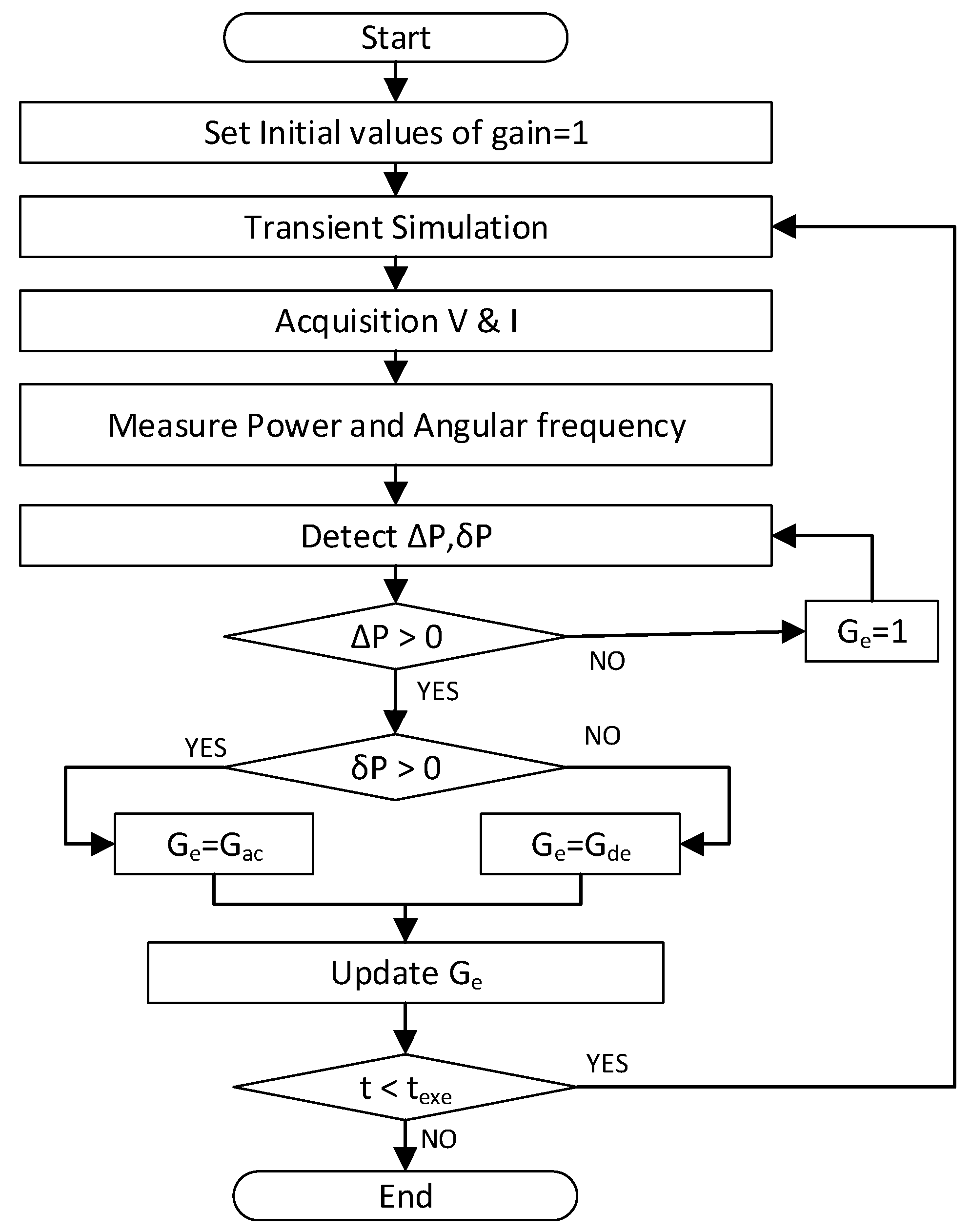
3.2. Flowchart
The flowchart of a bouncy control is shown in Figure 6. The system is initializing with and three phase voltages and currents are measured in a simulation through voltmeter and ammeter, respectively. In the actual system, the voltages and currents are first changed from abc-axis to dq-axis. However, in the flowchart, it is unnecessary to show a transformation. Power and frequency are acquired from the data obtained through measurement. The method of acquisition without using PLL is presented in [28]. Power and frequency are being measured continuously, so the change in power and () and derivate of power () can easily be detected. These parameters are the key factors in the execution of emergency control. The selecting criteria ’ from ‘’, and ‘’, can be seen in Table 1. The algorithm is designed to limit the contribution of power to the grid when the VSG reaches to its maximum power, therefore only is considered to change gains in a bouncy control, while the gain is unchanged at the time when (it can be introduced in future studies). When , it further detects the power derivative ‘’ to find out whether the curve is positive or negative. ‘texe’ is the time of execution of simulation, when the time ‘t’ is less than the execution time ‘texe’, the system keeps updating ‘’ in the simulation. Emergency control ends with the termination of the simulation.
3.3. Lyapunov Stability Analysis
The emergency power controller strategy is justified by implementing transient system analysis by using the online Lyapunov method. Evaluation of the Lyapunov function through transient simulation helps to calculate the energy function of the VSG, which in turn represents the stability of the system. It has few advantages over small signal state-space stability: (i) there is no need to solve non-linear differential equation of a system; (ii) no assumptions are required; and (iii) it does not change a system into linear, so it has accurate results. Due to these advantages, the Lyapunov method has been commonly used by researchers.
However, in the Lyapunov method, the main task is to find the Lyapunov function. It should be designed such that the function gives zero output value at a stable condition. The similar online optimization technique to improve control parameters by reducing the fitness value of an objective function; depending on the error of an electric parameters is presented in [29]. The Lyapunov function for a synchronous generator is presented in [18,25] by calculating the energy function. As VSG is a replica of synchronous generator, so this energy function could be implemented in VSG control.
where ‘V’ is the energy function of transient system when fault or any disturbance occurs. ‘’ is a power angle of VSG. ‘’ is the angle at stable point. Pin is the input reference power. ‘’ is the output electrical power. It can be seen from Equation (9), the energy function is divided into two sections: (i) kinetic energy ‘’, and (ii) potential energy ‘’. The kinetic energy is positive during oscillations, as the inertia and change in angular frequency is equal to or greater than zero. The potential energy has a negative sign, so the magnitude of a second term must be less than zero or the first term during oscillations; to satisfy .
The kinetic energy ‘’ is dependent on the variable ‘’–change in frequency, nominal frequency ‘’, and virtual inertia coefficient ‘J’. It can be assumed from the Equation (10), the kinetic energy is present in a system due to change in frequency ‘’, when the system is at the stable condition i.e., ; then ‘’, consequently there is no kinetic energy in a system (). It can be observed from Equation (4) that emergency gain ‘’ is influencing the derivative of ω, when the ‘’ increases the change in angular frequency also rises and vice versa. To enhance the angular frequency stability, it is better to take Ge less than 1, which in turn reduces the change in angular frequency.
The potential energy ‘’ is dependent on the power and the phase angle of VSG. When there is a phase difference in the VSG with respect to the grid, then there is an existence of potential energy in the system. The reference power angle ‘’ has basically ‘’ value at a grid. At the stable condition, is equal to , therefore the term () and () are equal to zero, consequently there is no more potential energy in a system . When the disturbance appears in a system, emergency gain is activated; it directly influences the potential energy of a system. The main purpose of implementing emergency gain is to provide the independent control during abnormal conditions of the VSG. As it can be seen from Equation (9), potential energy has a negative sign, therefore it causes declining behavior on the energy function. So, the increase in potential energy ‘’ causes the reduction in overall energy ‘’. Hence, it improves the responsiveness of a system. By contrast, when the emergency gain is set lower than 1 then the potential energy ‘’ falls, consequently, the overall energy takes a longer time to stabilize.
At the stable condition, the transient energy is supposed to be at zero. When any disturbance occurs in a system, the energy becomes positive that shows the system is under an abnormal condition. The derivative of the system transient energy must be negative to fulfill the Lyapunov stability criterion. The negative value shows that the transient system is returning back to the equilibrium state after the disturbance [18]. The derivative of ‘’ in Equation (9) is taken by considering the variable :
The above expression is a derivative equation of the system energy, it is necessary to be negative to show its decaying behavior (). The second term remains negative for , it is a damping factor. The first term of Equation (12) is negative when the system is approaching the equilibrium state. For the positive (), the derivative of is negative and for the negative , the derivative of is positive. Therefore, the first term maintains negative in either conditions.
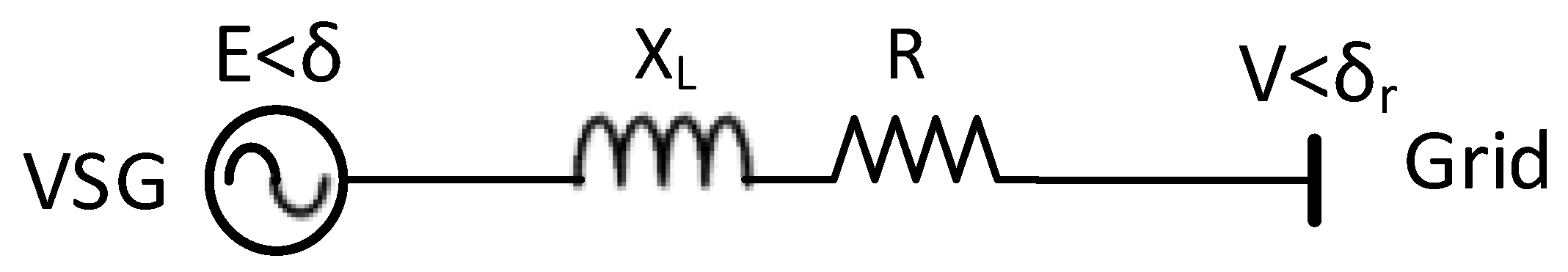
The interlinking of the VSG inverter with a grid is demonstrated in Figure 7. The voltage generated from the VSG is represented by , in which, is the amplitude of the voltage, while ‘’ is the power angle of voltage. is the instantaneous voltage of a grid, ’’ is the amplitude of the voltage and is the reference power angle of a grid which is ideally at ‘0’ (). and are the line impedances.
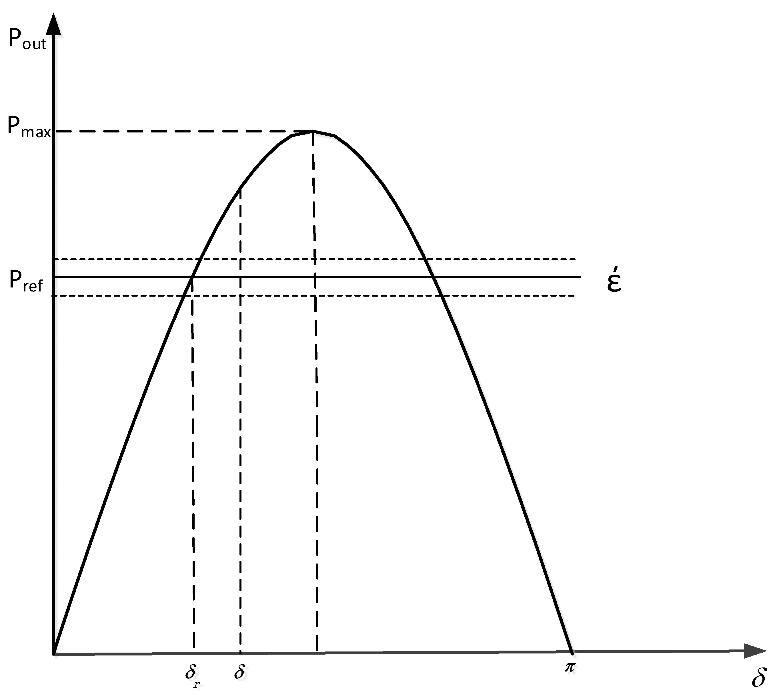
The angular frequency of a grid is taken as a reference angular frequency of the dq-axis. The power curve is presented in Figure 8. ‘’ is the power angle at which a reference power is providing to the system. is the maximum available power. is a power margin, power is considering stable within its limit.
4. VSG Interconnection with a Grid—Case 1
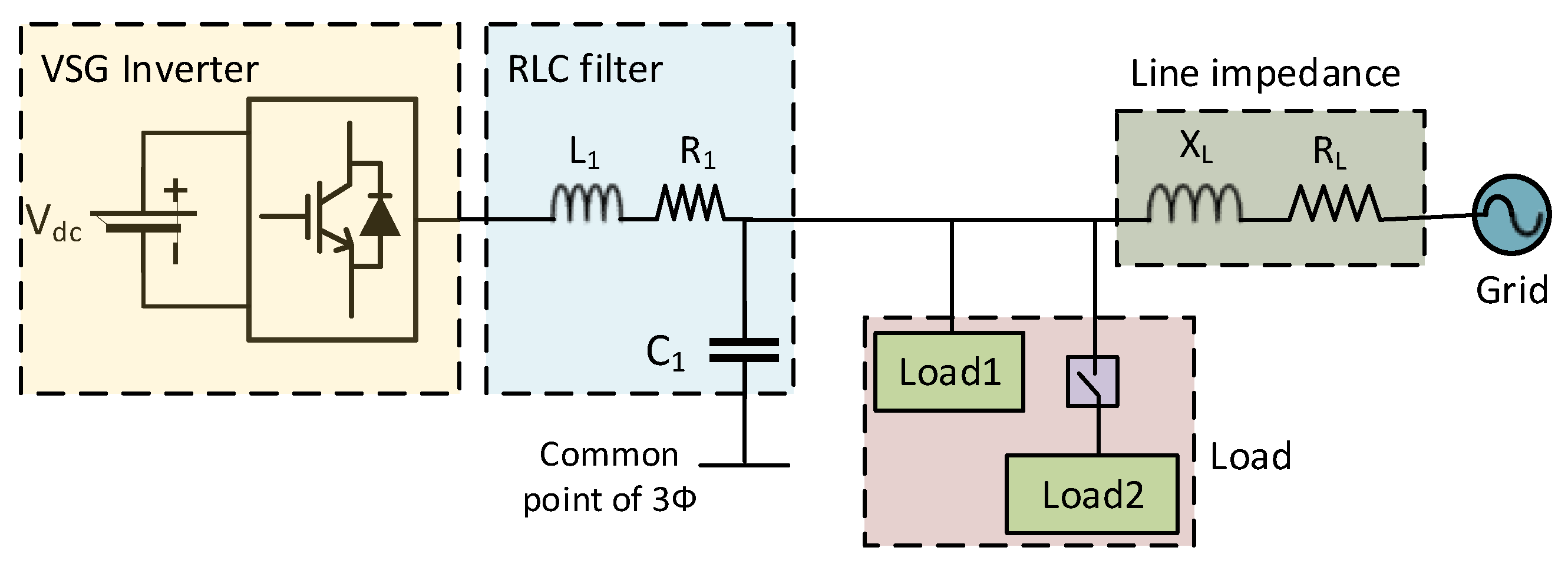
The system is designed for the VSG operating with renewable source and it is connected with a load and a grid in Figure 9. As the VSG is getting power through the renewable source, so it is necessary to deliver the maximum power through it. The load of 16 kW is connected near the VSG, the load is intentionally unevenly distributed among the VSG and the grid such that the VSG is providing power at its full capacity of 15,000 W, whereas the grid is contributing only 1000 W to the load. The additional load of 6 kW is added to the system at 0.6 s; after the system approaches stability. The disturbance caused due to the addition of this load is considered hereafter.
The emergency control is implemented on the VSG inverter to support the system during disturbance. The experiments are performed to show the behavior of the proposed bouncy control. The VSG is operating at its full load of 15 kW. The other parameters are presented in Table 2.
Impact of Gain in VSG System
This research focuses on the improvement of VSG stability under abnormal condition; by implementing emergency power control. The experiment is performed on a VSG-connected grid mode system to find out the impact of accelerating and decelerating emergency gain in the time of stabilization. A case of adding the load is considered to create instability in a system. The emergency accelerating gain is set to 1, while the power trend is carried out after applying different decelerating gain. The increase in Gde is shows improvement in the transition time.
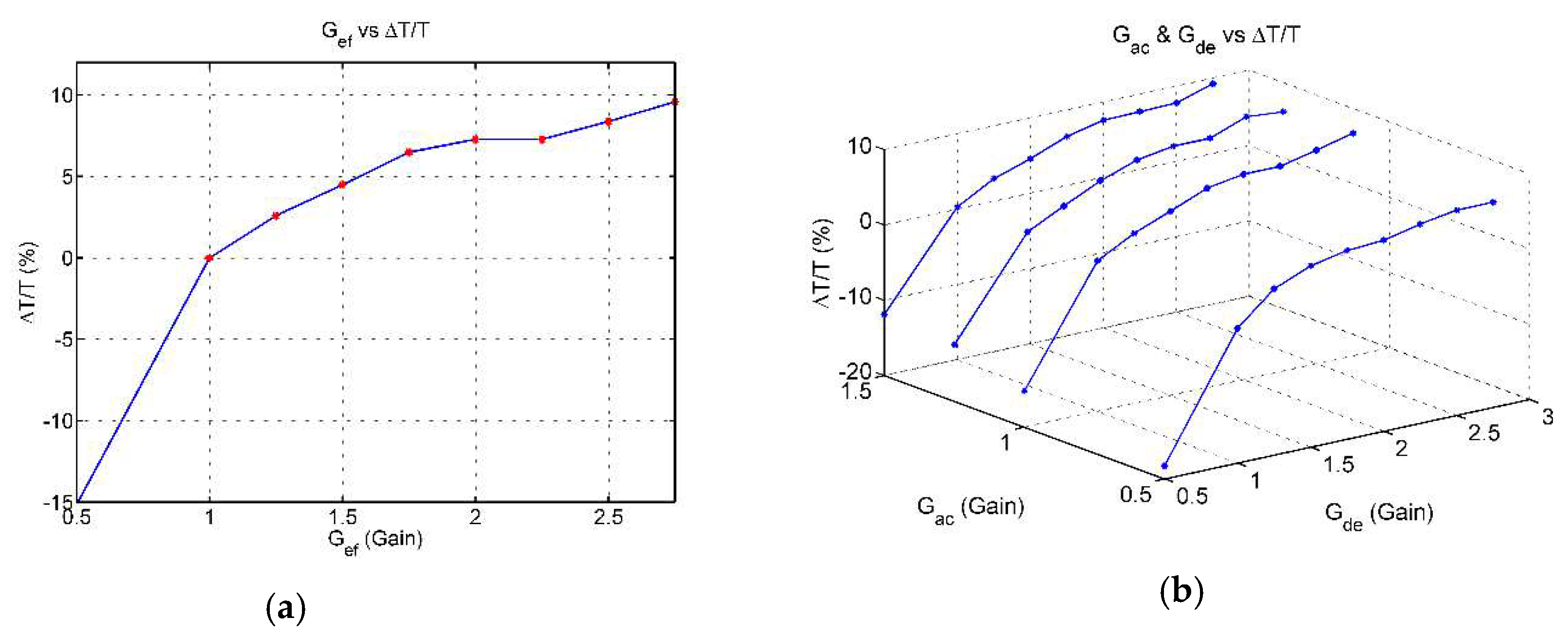
To elaborate the effect of and on a system, the graphs are plotted between the variation in gains and the ratio of change in settling time (). In Figure 10a, the two-dimensional graph between and , the rising curve shows the improvement in transition time on increasing . The experiment is carried out with the gains between 0.5–3. When the gain ‘ is set to 0.5, it is showing around 16% lapse in stabilizing time, while 2.5 and 2.75 are showing 9.6% and 10% improvement in transition time. Therefore, it is justified to choose the decelerating gain between 2.5–3 for the best performance of VSG during disturbance. In Figure 10b, the three-dimensional graph between and with . It can be observed through graph that has a negligible effect on transition time, but it is only effective and causing delay in transition time when the gain is <1.
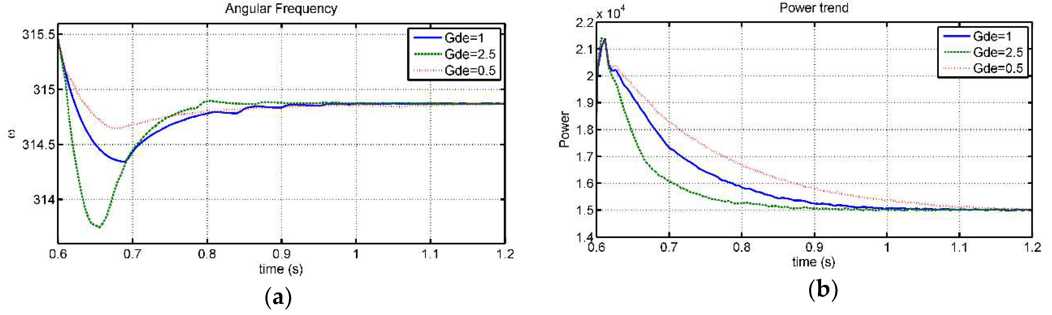
In this case, we are considering the significance of bouncy control. The bouncy control is adjusting the gain of power difference on the basis of change in power and the derivative of power. Implementing this control shows improvement in stability of the system. The Lyapunov stability analysis is done by using the energy function [18,25]. The trends of angular frequency generated through a proposed control from different gains during the time of disturbance are shown in Figure 11a. It can be noticed that the stabilization time of angular frequency from ‘ = 2.5’ is better than ‘ = 1’ (actual system), however, it causes the extreme frequency drop of 313.75 Hz/s (314.28 Hz/s in the actual system). It can be concluded that it is a tradeoff between time and maximum undershoot. The value of gain can be selected according to the angular frequency limit. In a case, when we want minimal dip in angular frequency, we can compromise on time by taking lower decelerating gain. When ‘ = 0.5’, it shows the least angular frequency dip of 314.64 Hz/s. It can be observed from Figure 11b that the power is stabilized earlier after disturbance when the gain is ‘ = 2.5’ in proposed control. It can also be seen through the power graph that the overshoot is same as before as the accelerating gain is not changing, only the transition time is improving. When the gain is lower than 1, the settling time increases. Hence, lower gain is beneficial for frequency stabilization, but it slows down the power response of the VSG.
It is worth noticing that the slower power response of VSG causes less influence on a grid for a limited time, which makes the VSG less effective toward any disturbance when it reaches its rated power. So, the VSG becomes robust, and it forces other sources of grid to contribute at that time.
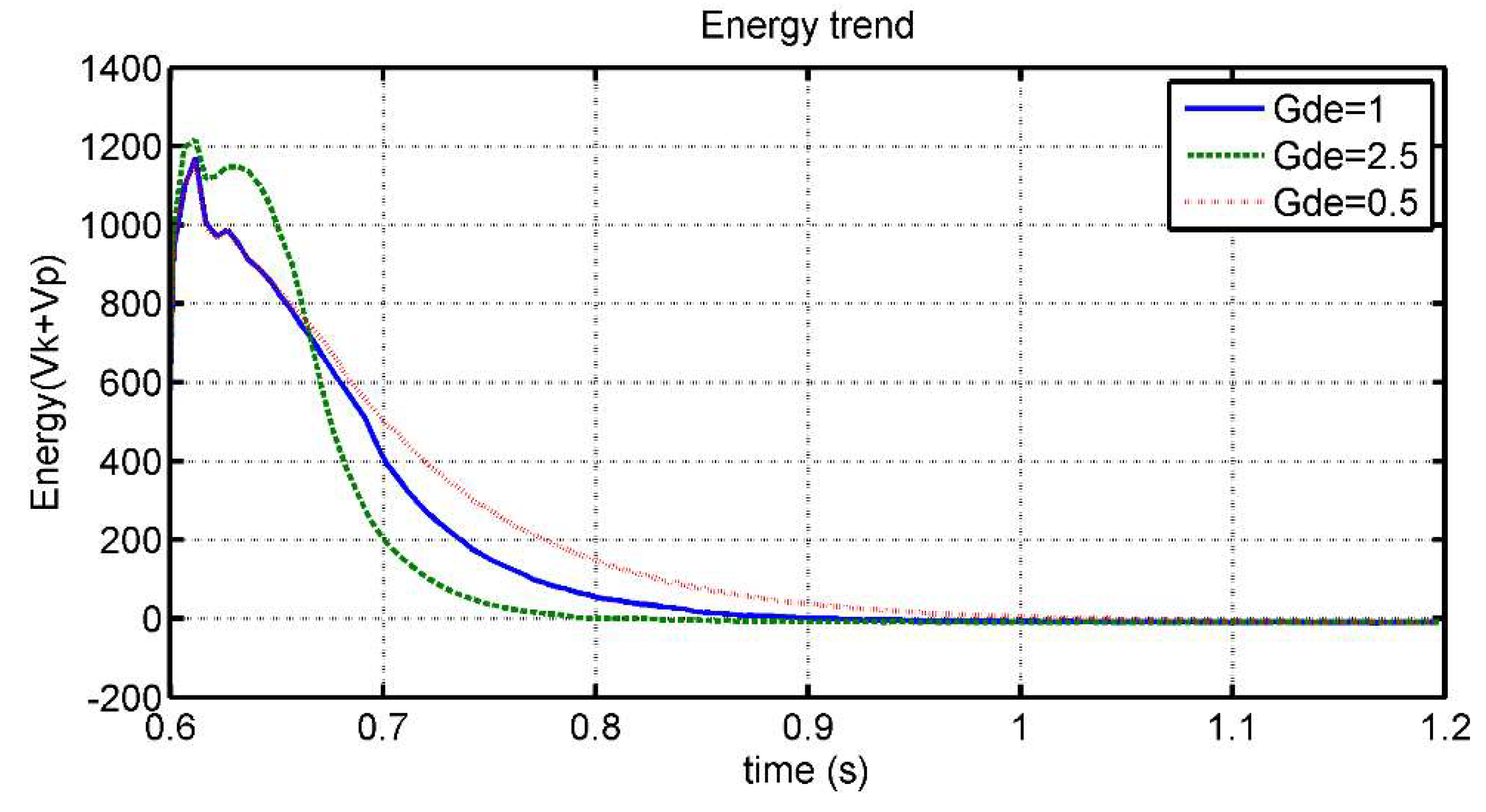
The energy graph to find the Lyapunov stability analysis in shown in Figure 12. The energy function used to find the fitness value of a system is a function of synchronous generator used by many researchers. The motive of using a synchronous generator’s energy function is obvious, as the VSG is its replica control. Hence, it is convenient to treat the VSG as a synchronous generator. It is clearly visible through graph that the system is returning to stable point by using proposed control. It shows that the kinetic energy is increased at the time of restoration of stability. On the contrary, the energy of proposed control is higher in the start for approximately 0.05 s, but its stew rate is higher, an therefore it achieves the steady state quickly.
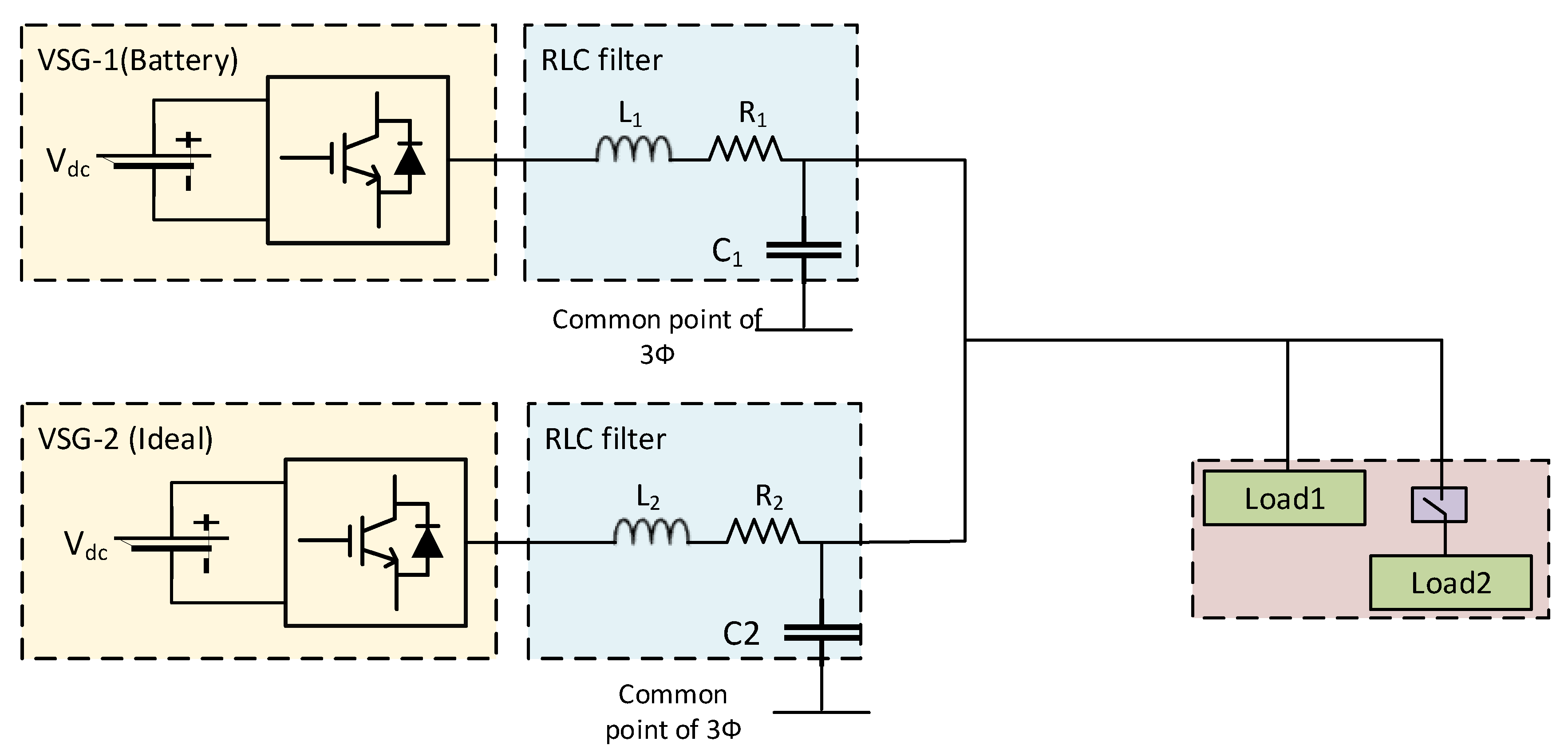
5. Multiple VSGs System (Island Microgrid)—Case 2
The bouncy control is implemented in a microgrid. The experiments are performed on a microgrid connected with two VSGs of the same power 15 kW, but different droop coefficient in Figure 13. The research on a microgrid of multiple VSGs system has been done by our research group in [30,31] PWM frequency for inverters is set to 5 kHz and values of resistance inductor capacitor (RLC) filters are calculated accordingly. The system is designed to generate three-phase AC voltage. The input direct current (DC) voltage is set to 800 V, while it is generating 380 V phase-phase-rms voltage at frequency of 50 Hz. The simulation is started with a load of 15,000 W and additional load of 15 kW is adding at 0.5 s.
Table 3 shows the parameters selected for the two VSGs. The droop coefficient of VSG1 is set to 10; four times less than the value set for VSG2. The different values are set to share different power from two VSGs utilizing more power of VSG1 when the load is less.
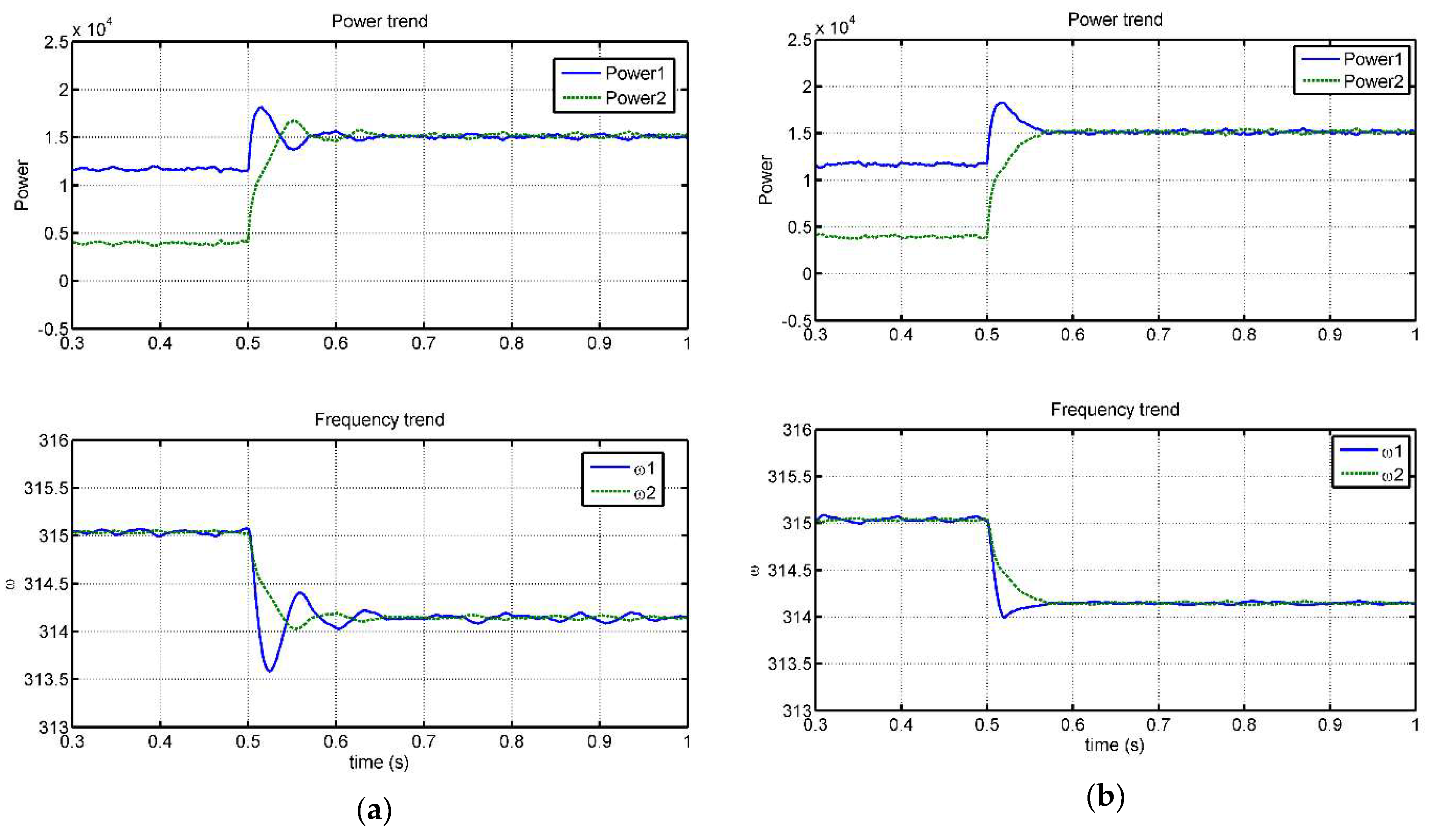
5.1. Loading/Unloading Analysis
At the time of addition of load, the VSG2 takes over the control to stabilize the system. Initially, when the load is 15 kW, the VSG1 and VSG2 are contributing 12 kW and 3 kW, respectively. As the load increases to 30 kW at 0.5 s, VSG1 contributes 3 kW to an additional load, whereas VSG2 supplies 12 kW. Overall, both VSGs start operating at full capacity of 15 kW. The transition of power and frequency due to the addition of load in the initial system (without emergency control) is shown in Figure 14a. The system shows instability in both parameters under observation (P, ω) and taking substantial time in settling as shown in Figure 14a. The angular frequency of VSG1 drops down to 313.6 Hz/s and settles at around 0.65 s.
The power and frequency graphs of a system; operating with bouncy control, are shown in Figure 14b. The bouncy control is introduced in VSG1 such that power error is operating at 50% sensitivity at the time of acceleration and 10% at the time of deceleration. The difference between accelerating and decelerating gain (sensitivity) are set closer. If the difference would be higher, then the VSG could show a variation in frequency while stabilizing. The controller is limiting the effect of a disturbance on VSG1 and forcing VSG2 to stabilize the system. The angular frequency drops down to 314 Hz/s and stabilizes at about 0.56 s. In this way, VSG1 becomes robust which in turn makes a microgrid strong. It can be observed that the bouncing in Figure 14a has significantly been reduced in Figure 14b. Moreover, the angular frequency of VSG1 drops down to around 313.5 Hz/s in Figure 14a, which is now improved to great extent (not showing undershoot in angular frequency).
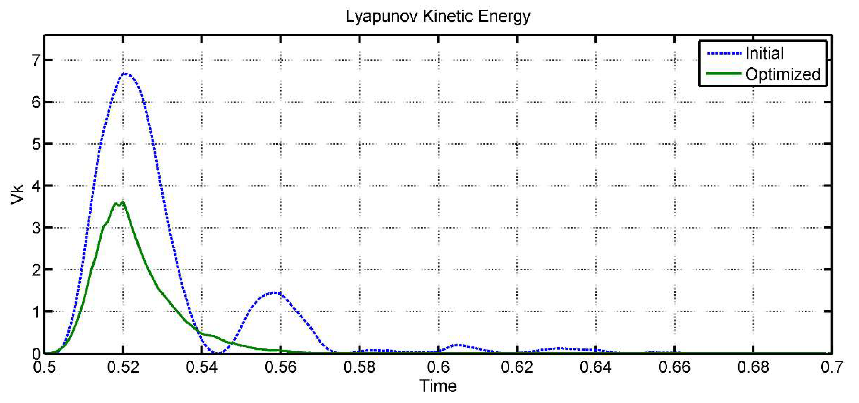
Lyapunov stability analysis is carried-out at VSG1 inverter control. The kinetic energy of Lyapunov function is associated with the angular frequency, so in this case, Equation (10) is being considered because the stability of VSG is majorly dependent on the angular frequency. It can be seen from Figure 15 that the peak energy of an initial system is almost double that of the optimized system which has bouncy control. Initial system is showing more oscillations and taking longer time to stabilize at around 0.65 s, whereas the optimized system is not showing oscillations; however it is showing relatively slower transient time at the start, but its overall stabilizing time is better than initial system i.e., 0.565 s. This control is limiting the instability of a system and suppressing the frequency oscillations.
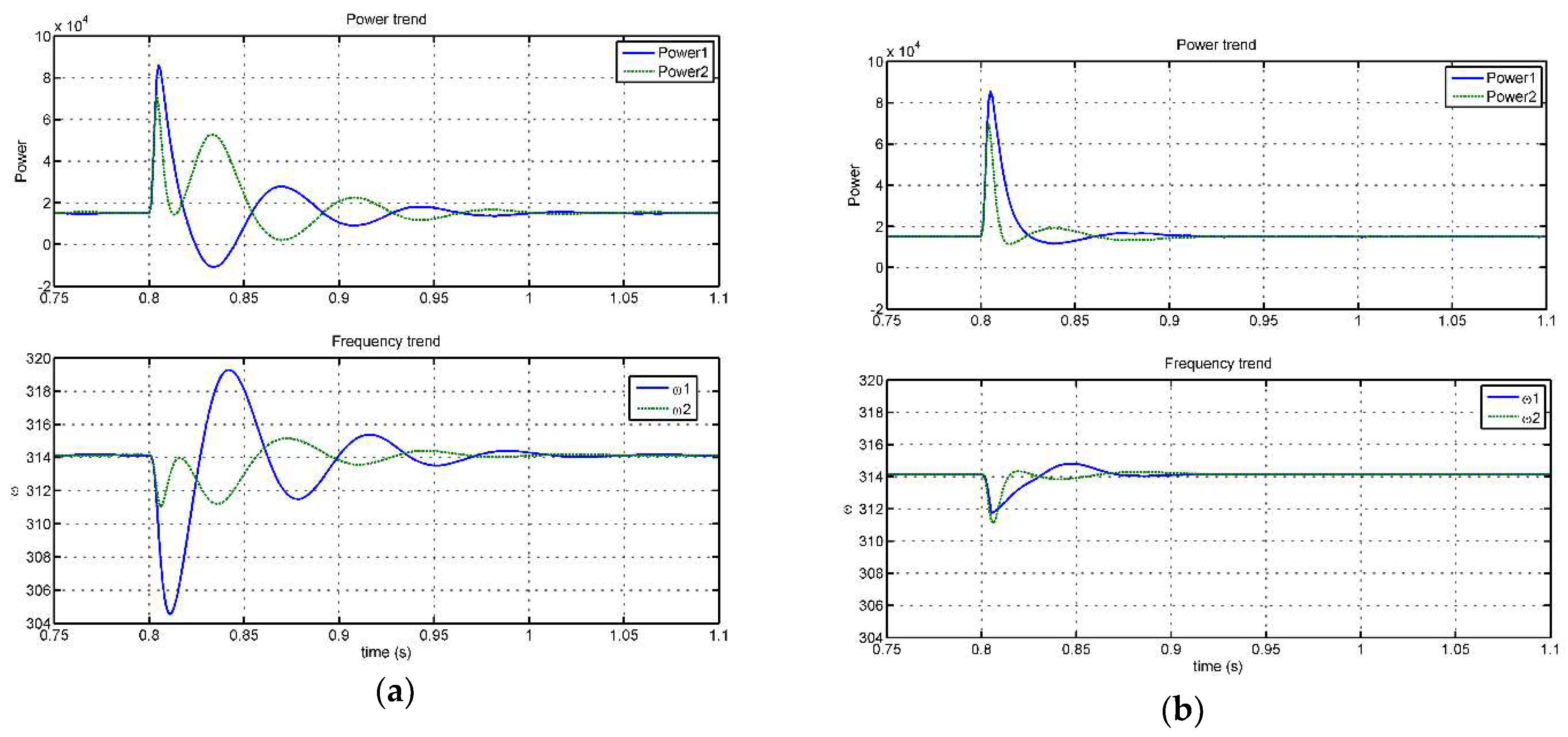
5.2. Fault Analysis
Three phase to ground fault is applied at 0.8 s for 0.01 seconds. The effects of initial and proposed control on recovery from the fault are analyzed as shown in Figure 16. The power and angular frequency oscillation is alleviated at around 0.9 s by using the proposed controller compared to 1 s by the initial controller. The proposed method can stabilize the system faster after the fault, by increasing the damping effect using emergency gain. It can be observed from Figure 16 that the power transient is initially showing a same trend for both controllers, because the proposed controller takes some time to respond, whereas a significant improvement can be seen in angular frequency of VSG-1. The undershoot of angular frequency has been reduced because the bouncy control is reducing the derivative of change in angular frequency by implementing emergency gain <1 in Equation (6), consequently, the oscillations are reduced and the system is brought back to the equilibrium state faster. The results show that the proposed controller is not only effective under a minor disturbance like loading or unloading, but it is also effective for limiting a fault-related disturbance. The limitation of this control method is a power sensing delay. It is observed from fault analysis, the peak power of the proposed controller during fault is same as the initial controller. However, there is a significant improvement in the frequency undershoot and the time to reach steady state.
6. Conclusions
In this paper, the emergency control of a virtual synchronous generator is introduced. A technique of bouncy control is implemented to improve the stability of a system by increasing or reducing the sensitivity of a system during recovery time. After using the proposed control, it is observed that the VSG is showing better response after a disturbance. The parameter ‘’ in bouncy control can make a system robust according to the system’s requirement. The criteria of selecting gain solely depends on the system’s strength. When the system has not enough strength to bear the disturbance, the small value of is used; that delays transition time while ensuring the minimal disturbance in VSG frequency. In another case, when the system is stronger, then the higher value of decelerating gain improves the stabilizing time. This controller makes the weakest source of a microgrid stronger by limiting its dependence on a load and a grid for a limited time that in turn gives a signal to other sources to contribute during that time. Hence, the overall system strengthens. The results are deliberated through power and frequency graphs. VSG stability is investigated through simulation-based Lyapunov stability analysis by executing energy function to verify the effectiveness of a control. The results show a markedly improved response. The stability can further be improved by increasing the power response of other VSG-controlled sources when its operating power is less than the rated power at the time of loading/unloading. The bouncy control can be used in any system, as it has a capability to make the system more robust. The coordination of multiple VSGs connected in parallel, particularly the island microgrid, can be greatly enhanced by using the bouncy control technique.
Author Contributions
Each author contributed extensively to the preparation of this manuscript. A.R. and X.Y. designed and developed the main research work, including designing and the controller, simulation model, analysis of the obtained results and writing original draft. H.R. proposed the lyapunov stability analysis method. H.G. and M.A. provided some useful suggestions in the construction of paper. All the authors revised and approved the publication.
Funding
This paper was supported by the Hebei Natural Science Funding (E2018502134); Liaoning Power Grid Corporation’s 2018 Science and Technology Project “Research on the Reactive Power and Voltage Optimization Strategy and Evaluation Index Considering Source and Load Fluctuation Characteristics”.
Acknowledgments
The author, A.R., would like to thank China Scholarship Council (CSC) for providing the funding during his PhD studies and Goldwind Science and Technology, Co. Ltd. for arranging the internship in their company.
Conflicts of Interest
The authors declare no conflict of interest
References
- Zhong, Q.C. Power-electronics-enabled autonomous power systems: Architecture and technical routes. IEEE Trans. Ind. Electron. 2017, 64, 5907–5918. [Google Scholar] [CrossRef]
- Jia, L.; Miura, Y.; Ise, T. Dynamic characteristics and stability comparisons between virtual synchronous generator and droop control in inverter-based distributed generators. In Proceedings of the 2014 International Power Electronics Conference (IPEC-Hiroshima 2014 - ECCE ASIA), Hiroshima, Japan, 18–21 May 2014. [Google Scholar]
- Guan, M.; Pan, W.; Zhang, J.; Hao, Q.; Cheng, J.; Zheng, X. Synchronous generator emulation control strategy for voltage source converter (vsc) stations. IEEE Trans. Power Syst. 2015, 30, 3093–3101. [Google Scholar] [CrossRef]
- Guerrero, J.M.; Vasquez, J.C.; Matas, J.; de Vicuna, L.G.; Castilla, M. Hierarchical control of droop-controlled ac and dc microgrids—a general approach toward standardization. IEEE Trans. Ind. Electr. 2011, 58, 158–172. [Google Scholar] [CrossRef]
- Hashmi, K.; Muhammad, M.K.; Jiang, H.; Muhammad, U.S.; Salman, H.; Muhammad, T.F.; Tang, H. A virtual micro-islanding-based control paradigm for renewable microgrids. Electronics 2018, 7, 105. [Google Scholar] [CrossRef]
- Bevrani, H.; Watanabe, M.Y. Mitani, Power System Monitoring and Control. Electron. Power 1981, 27. [Google Scholar] [CrossRef]
- Brabandere, K.D.; Bruno, B.; van den Keybus, J.; Woyte, A.; Driesen, J.; Belmans, R. A Voltage and Frequency Droop Control. Method for Parallel Inverters. IEEE Trans. Ind. Electron. 2007, 22, 1107–1115. [Google Scholar]
- Nikkhajoei, H.; Lasseter, R.H. Distributed Generation Interface to the CERTS Microgrid. IEEE Trans. Power Deliv. 2009, 24, 1598–1608. [Google Scholar] [CrossRef]
- Vandoorn, T.L.; Meersman, B.; De Kooning, J.D.M. Analogy Between Conventional Grid Control and Islanded Microgrid Control Based on a Global DC-Link Voltage Droop. IEEE Trans. Power Deliv. 2012, 27, 1405–1414. [Google Scholar] [CrossRef] [Green Version]
- Chandorkar, M.C.; Divan, D.M.; Adapa, R. Control of parallel connected inverters in standalone ac supply systems. IEEE Trans. Ind. Appl. 1993, 29, 136–143. [Google Scholar] [CrossRef]
- Driesen, J.; Visscher, K. Virtual synchronous generators. In Proceedings of the 2008 IEEE Power and Energy Society General Meeting-Conversion and Delivery of Electrical Energy in the 21st Century, Pittsburgh, PA, USA, 20–24 July 2008. [Google Scholar]
- Hirase, Y.; Noro, O.; Yoshimura, E.; Nakagawa, H.; Sakimoto, K.; Shindo, Y. Virtual synchronous generator control with double decoupled synchronous reference frame for single-phase inverter. In Proceedings of the 2014 International Power Electronics Conference (IPEC-Hiroshima 2014-ECCE ASIA), Hiroshima, Japan; 18–21 May 2014. [Google Scholar]
- Chen, Y.; Hesse, R.; Turschner, D.; Beck, H.-P. Improving the grid power quality using virtual synchronous machines. In Proceedings of the 2011 International Conference on Power Engineering, Energy and Electrical Drives, Malaga, Spain, 11–13 May 2011. [Google Scholar]
- Beck, H.-P.; Hesse, R. Virtual synchronous machine. In Proceedings of the 2007 9th International Conference on Electrical Power Quality and Utilisation, Barcelona, Spain, 9–11 October 2007. [Google Scholar]
- Zhong, Q.-C.; Weiss, G. Synchronverters: Inverters that mimic synchronous generators. IEEE Trans. Ind. Electron. 2011, 58, 1259–1267. [Google Scholar] [CrossRef]
- Liu, J.; Miura, Y.; Bevrani, H.; Ise, T. Enhanced virtual synchronous generator control for parallel inverters in microgrids. IEEE Trans. Smart Grid 2016, 1–10. [Google Scholar] [CrossRef]
- Ma, Y.; Lin, Z.; Yu, R.; Zhao, S. Research on improved VSG control algorithm bsed on capacity-limited energy storage system. Energies 2018, 11, 677. [Google Scholar] [CrossRef]
- Alipoor, J.; Miura, Y.; Ise, T. Power system stabilization using virtual synchronous generator with alternating moment of inertia. IEEE J. Emergg Top. Power Electron. 2015, 3, 451–458. [Google Scholar] [CrossRef]
- Cheng, C.; Zeng, Z.; Yang, H. Wireless parallel control of three-phase inverters based on virtual synchronous generator theory. In Proceedings of the 17th International Conference on Electrical Machines and Systems (ICEMS), Hangzhou, China, 22–25 October 2014. [Google Scholar]
- Shintai, T.; Miura, Y.; Ise, T. Oscillation Damping of a Distributed Generator Using a Virtual Synchronous Generator. IEEE Trans. Power Deliv. 2014, 29, 668–676. [Google Scholar] [CrossRef]
- Paquette, A.D.; Reno, M.J.; Harley, R.G. Sharing Transient Loads: Causes of Unequal Transient Load Sharing in Islanded Microgrid Operation. IEEE Ind. Appl. Mag. 2014, 20, 23–34. [Google Scholar] [CrossRef]
- Fan, W.; Yan, X.; Hua, T. Adaptive parameter control strategy of VSG for improving system transient stability. In Proceedings of the Future Energy Electronics Conference and ECCE Asia (IFEEC 2017-ECCE Asia), 2017 IEEE 3rd International, Kaohsiung, Taiwan, 3–7 June 2017. [Google Scholar]
- Yu, B. An improved frequency measurement method from the digital PLL structure for single-phase grid-connected PV applications. Electronics 2018, 7, 150. [Google Scholar] [CrossRef]
- Li, M.; Huang, W.; Tai, N.; Yu, M. Lyapunov-Based Large Signal. Stability Assessment for VSG Controlled Inverter-Interfaced Distributed Generators. Energies 2018, 11, 2273. [Google Scholar] [CrossRef]
- Machowski, J.; Gubina, F.; Omahen, P. Power system transient stability studies by Lyapunov method using coherency based aggregation. In Proceedings of the Power systems and power plant control proceedings of the IFAC symposium, Beijing, China, 12–15 August 1986. [Google Scholar]
- Yan, X.; Zhang, X.; Zhang, B.; Ma, Y.; Wu, M. Research on distributed PV storage virtual synchronous generator system and its static frequency characteristic analysis. Appl. Sci. 2018, 8, 532. [Google Scholar] [CrossRef]
- Zhang, B.; Yan, Y.; Li, D.; Zhang, X.; Han, J.; Xiao, X. Stable Operation and Small-Signal. Analysis of Multiple Parallel DG Inverters Based on a Virtual Synchronous Generator Scheme. Energies 2018, 11, 203. [Google Scholar] [CrossRef]
- Elsayad, M.A.; Sarhan, G.; Abdin, A.M.; Mohamed, H.S. Power Angle Control of Virtual Synchronous Generator. J. Electr. Eng. 2017, 17. Available online: http://www.jee.ro/covers/editions.php?act=art&art=WG1471637795W57b76923d7215 (accessed on 15 September 2018).
- Aazim, R.; Liu, C.; Haaris, R.; Mansoor, A. Rapid generation of control parameters of Multi-Infeed system through online simulation. Ingeniería e Investigación 2017, 37, 67–73. [Google Scholar] [CrossRef]
- Zhang, B.; Yan, X.; Altahir, S.Y. Control design and small-signal modeling of multi-parallel virtual synchronous generators. In Proceedings of the Compatibility, Power Electronics and Power Engineering (CPE-POWERENG), 2017 11th IEEE International Conference, Russia, Moscow, 20–22 September 2017. [Google Scholar]
- Altahir, S.Y.; Yan, X.; Gadaalla, A.S. New Control. Scheme for Virtual Synchronous Generators of Different Capacities. In Proceedings of the Energy Internet (ICEI), IEEE International Conference, Beijing, China, 17–21 April 2017. [Google Scholar]
Figure 1.
Transition to island microgrid.

Figure 2.
Angular frequency and active power control of a virtual synchronous generator (VSG).

Figure 3.
Voltage and reactive power control of VSG.

Figure 4.
Overall control of grid-connected VSG.

Figure 5.
Emergency control of VSG.

Figure 6.
Flowchart of bouncy control.

Figure 7.
Interconnection of VSG with a grid.

Figure 8.
Power curve of VSG.

Figure 9.
Single VSG inverter connecting with a load and a grid.

Figure 10.
The relation of gain to transition time ratio: (a) gain vs ΔT/Ts*, (b) Gac and Gde vs ΔT/Ts*.
Figure 10.
The relation of gain to transition time ratio: (a) gain vs ΔT/Ts*, (b) Gac and Gde vs ΔT/Ts*.

Figure 11.
The trends of measured angular frequency and active power on different decelerating gains: (a) angular frequency trend, (b) active power trend.
Figure 11.
The trends of measured angular frequency and active power on different decelerating gains: (a) angular frequency trend, (b) active power trend.

Figure 12.
The trend of the energy function of Lyapunov stability.

Figure 13.
Multiple VSGs connected in parallel (island microgrid).

Figure 14.
The result of the frequency and power curves. (a) Initial curves, (b) optimized curves.

Figure 15.
Lyapunov kinetic energy trend of VSG-1.

Figure 16.
The result of the frequency and power curves under a fault condition. (a) Initial curves, (b) optimized curves.
Figure 16.
The result of the frequency and power curves under a fault condition. (a) Initial curves, (b) optimized curves.


Table 1.
Bouncy control of gain selector.
| ΔP (P-Pref) | d(P)/dt | Slope | |
|---|---|---|---|
| ΔP> 0 | d(P)/dt<0 | Decelerating | |
| ΔP> 0 | d(P)/dt>0 | Accelerating | |
| ΔP< 0 | d(P)/dt<0 | Accelerating | 1 |
| ΔP< 0 | d(P)/dt>0 | Decelerating | 1 |
Table 2.
Parameter of a system for case 1.
| Parameters | Values | Parameters | Values |
|---|---|---|---|
| Sbase | 15 kW | fpwm | 5000 Hz |
| V* | 380 V | VL-N | 220 V |
| ω | 2π × 50 Hz/s | Gde | 0.5 & 2.5 |
| D | 10 | Gac | 1 |
| Load2 | 6 kW | L1 | 1.5 mH |
| fn | 50 Hz | C1 | 150 μF |
| Vdc | 800 V | J | 0.1 |
| n | 0.016 | R1 | 0.05 Ω |
| XL | 0.3mΩ | RL | 0.1 Ω |
Table 3.
Parameter of a system.
| Parameters | Values | Parameters | Values |
|---|---|---|---|
| Sbase- | 15 kW | fpwm | 5000 Hz |
| V* | 380 V | VL-N | 220 V |
| ω | 2π x 50 Hz/s | Gde | 10% |
| fn | 50 Hz | Gac | 50% |
| D(VSG-1) | 10 | R1 | 0.05 Ω |
| D(VSG-2) | 40 | L1 | 2.38 mH |
| Load2 | 15 kW | C1 | 170 µF |
| Load1 | 15 kW | R2 | 0.05 Ω |
| Vdc | 800 V | L2 | 2.38 mH |
| n | 0.010 | C2 | 170 µF |
| J1 | 0.1 | J2 | 0.1 |
© 2018 by the authors. Licensee MDPI, Basel, Switzerland. This article is an open access article distributed under the terms and conditions of the Creative Commons Attribution (CC BY) license (http://creativecommons.org/licenses/by/4.0/).
Share and Cite
MDPI and ACS Style
Rasool, A.; Yan, X.; Rasool, H.; Guo, H.; Asif, M. VSG Stability and Coordination Enhancement under Emergency Condition. Electronics 2018, 7, 202. https://doi.org/10.3390/electronics7090202
AMA Style
Rasool A, Yan X, Rasool H, Guo H, Asif M. VSG Stability and Coordination Enhancement under Emergency Condition. Electronics. 2018; 7(9):202. https://doi.org/10.3390/electronics7090202
Chicago/Turabian StyleRasool, Aazim, Xiangwu Yan, Haaris Rasool, Hongxia Guo, and Mansoor Asif. 2018. "VSG Stability and Coordination Enhancement under Emergency Condition" Electronics 7, no. 9: 202. https://doi.org/10.3390/electronics7090202
Note that from the first issue of 2016, this journal uses article numbers instead of page numbers. See further details here.