1. Introduction
The Compton wavelength gives the minimum radius within which the mass of a particle may be localized due to relativistic quantum effects, neglecting the particle’s self-gravity, while the Schwarzschild radius gives the maximum radius within which the mass of a black hole may be localized due to classical relativistic gravity, neglecting quantum effects. In a mass-radius diagram, the two lines intersect near the Planck point , where denotes the Planck mass and the Planck length, so that relativistic-quantum-gravitational effects become significant in this region. In addition, the equivalence of the Compton and Schwarzschild radii close to the Planck scales suggests that a final theory of quantum gravity (QG) should yield a unified description of fundamental particles and black holes. Nonetheless, how such a unification could be achieved may be considered an outstanding problem for both elementary particle physics, and the physics of black holes, even in the absence of a final theory.
Since canonical non-gravitational QM and quantum field theories (QFTs) are based on the concept of wave-particle duality, encapsulated in the de Broglie relations, these may break down close to . However, it is unclear what (if any) physical interpretation can be given to quantum particles with energies , since these correspond to “matter waves” with sub-Planckian wavelengths and time periods (), according to canonical quantum dispersion relations. On the other hand, “particles” with rest masses have sub-Planckian Compton wavelengths, , but super-Planckian Schwarzschild radii, , and may be interpreted as black holes. We therefore propose corrections to the standard de Broglie relations, which are valid in the semi-Newtonian limit, allowing them to be extended into the region .
Here, the semi-Newtonian theory is defined as the Newtonian limit of general relativity, in which space and time are absolute but there exists a cosmic speed limit , which must be imposed “by hand” on the quantum sector. Though, from the viewpoint of a final theory, this is clearly inadequate, it has the advantage of allowing us to describe key phenomenological features of spherically symmetric systems on both halves on the mass-radius diagram, and , within a unified ontological framework. In other words, using the same set of assumptions about the nature of space and time, the finite speed of light, and the form of the quantum dispersion relations, we recover well-known features of both canonical QM and classical gravity. These assumptions give rise to both a modified Schrödinger equation and a modified expression for the Compton wavelength. Both reduce to the standard forms for , as required for consistency, but, crucially, also allow us to recover the standard expression for the Schwarzschild radius for , using standard “quantum” arguments. Thus, we interpret the additional terms in the modified de Broglie relations, which involve all three fundamental constants, G, c and ℏ, as representing the self-gravitation of the wave packet in the semi-Newtonian background.
The structure of this paper is as follows. In
Section 2, we review the basic arguments for the “quantum” nature of non-relativistic point-particles and relativistic fields, focussing on the equivalence of wave-particle duality, as expressed via the canonical dispersion relations, and formal quantization schemes. In
Section 3.1, we briefly review Newtonian gravity and general relativity, with special emphasis on their application to spherically symmetric bodies (i.e., particles and black holes). The gravitational implications of the the semi-Newtonian approximation are discussed in
Section 3.2.
Section 3.3 considers two previous attempts to incorporate quantum effects into gravitational theories, the Schrödinger-Newton equation and Loop Quantum Gravity (LQG). Their relations to the extended de Broglie theory, and to the problem of obtaining a unified description of fundamental particles and black holes, are also discussed. In
Section 3.4, the quantum mechanical implications of the semi-Newtonian approximation are considered and the conceptual framework for the extended de Broglie theory is defined. The Ansatz for the extended relations is motivated by considering the asymptotic black hole regime in
Section 4.1 and the full relations are presented in
Section 4.2. In
Section 5, we determine the equations of motion (EOM) for the quantum state and the associated Hamiltonian and momentum operators, in both the particle and black hole regimes. The implications of the extended theory for the Hawking temperature are discussed in
Section 6, and alternative unification schemes for black holes and fundamental particles, based on Generalized Uncertainty Principle (GUP) phenomenology, are considered in
Section 7, with special emphasis on how these relate to the ideas discussed in
Section 2,
Section 3,
Section 4,
Section 5 and
Section 6. A brief summary our our main results is given in
Section 8. For reference, the four postulates of canonical QM are listed in the
Appendix.
Thus, the results presented in
Section 2 and
Section 3 are mostly pedagogical, while those presented in
Section 4,
Section 5 and
Section 6 are based primarily on results obtained in [
1], in which the extended de Broglie theory was first introduced. However, the purpose of the present work is not simply to review the results of previous studies, but to propose a provisional answer to the questions posed in the title, “Which quantum theory must be reconciled with gravity? (And what does it mean for black holes?)”, which may be considered important open questions in black hole physics. For this reason, the material presented in
Section 2 and
Section 3 is chosen to highlight the steps required to obtain a unified ontology for the description of black holes and fundamental particles. Since this
necessarily entails important modifications to our existing notions of what makes a theory “quantum”, it leads naturally to the extended de Broglie theory as a
provisional scheme for unification in the semi-Newtonian limit. Throughout, we explore the relation between this theory and existing models of modified quantum theory—relativistic, non-relativistic and semi-relativistic—motivated by gravitational considerations. In each case, we attempt to clarify the theoretical assumptions underpinning different approaches and to identify which (if any) of the physical assumptions on which different models are based may be in contradiction with one another. In particular, special emphasis is given to particle-black hole unification schemes arising in the context of GUP phenomenology, which are considered in detail in
Section 7.
2. What Makes a Theory “Quantum”?
The essence of quantum theory is wave-particle duality. Though, philosophically, a somewhat slippery concept [
2], it is encapsulated mathematically in a very precise form via the de Broglie relations [
3]
In 1924, de Broglie’s great insight was to relate the constants of motion of a classical point particle, energy
E and momentum
, with properties hitherto associated only with waves; frequency
f and wavelength
λ, or, equivalently, angular frequency
and wave number
. This was made possible by Planck’s earlier discovery of new fundamental constant with dimensions of action,
, which proved necessary to explain the observed spectrum of black body radiation. The quantization of absorbed and emitted radiation, according to Equation (2.1), was able to account for the suppression of high-energy modes that otherwise result in an “ultraviolet catastrophe” [
4].
The breakthrough leading, ultimately, to the development of modern quantum mechanics (QM) and quantum field theory (QFT) came when de Broglie proposed that the relations (2.1) were applicable to all forms of matter and radiation. Thus, the foundation of any quantum theory is the quantum dispersion relation, which is obtained by substituting (2.1) into the classical relation between E and . In general, this may be relativistic or non-relativistic and may apply to objects with zero or nonzero rest mass. Typically, the latter are considered “particles” in the classical theory and acquire wave-like characteristics via quantization, whereas the former are considered classically as “waves”, which acquire particle-like properties via (2.1). The equation of motion (EOM) for the quantum state must satisfy the dispersion relation obtained by combining the classical energy-momentum relation with the de Broglie relations and be invariant under the symmetries of the corresponding classical theory.
For massive particles, the quantum dispersion relation involves ℏ and will also include c, the speed of light, if the theory is relativistic. Roughly speaking, we may say that a theory describing massive particles is quantum (meaning it incorporates wave-particle duality) and non-relativistic if its dispersion relation contains, ℏ but not c, and if the resulting EOM are invariant under rotations, translations in time and space, and local Gallilean boosts. Likewise, a theory of massive particles is quantum and relativistic if its dispersion relation contains both ℏ and c, and if the resulting EOM are invariant under the action of the Poincáre group, comprising rotations, translations and local Lorentz boosts.
2.1. Wave-Particle Duality in Newtonian Space—Without Newtonian Gravity
The non-relativistic energy-momentum relation is
where
represents an external classical potential, not generated by the particle itself. The quantum dispersion relation is, therefore,
By assuming that a single “matter wave” mode, corresponding to a single value of the classical momentum
, is given by
, and that a general quantum state
is given by a superposition of modes, the next fundamental breakthrough was made by Schrödinger, who obtained the EOM for a non-relativistic quantum system:
For a given V, this equation is unique and, hence, is the only EOM consistent with Equations (2.1) and (2.2). The operator is called the Hamiltonian and its eigenvalues represent the possible results of measurements of the system’s energy.
In the position space representation, the results of position measurements are given by the classical position vector, so that the operators corresponding to classical canonical coordinates are given by
with eigenfuctions
The equivalents of Equations (2.5) and (2.6) in the momentum space representation are obtained by applying the transformation
, so that the position and momentum operators obey the canonical commutation relations,
in either representation. In general, consistency requires that these hold in
any representation, so that (2.7) may be taken as a definition: any pair of operators satisfying the canonical commutation relations are valid representations of
and
. It is a fundamental postulate of canonical QM that operators representing other dynamical variables bear the same functional relation to these as do the corresponding classical quantities to the classical position and momentum [
3].
In the Schrödinger picture, operators representing physical observables are time-independent, whereas the quantum state
ψ is time-dependent, according to
Equivalently, in the Heisenberg picture, operators are time-dependent and states time-independent, so that
and the quantum EOM becomes
Equation (2.10) takes exactly the same form as the Hamilton-Jacobi equation in classical non-relativistic mechanics [
5] under the transformation
where
is the classical Poisson bracket for the functions
,
. (The Schrödinger equation may also be related to Hamilton’s equation via the transformation
, where
is the action.) In classical mechanics, the Poisson bracket for the canonical coordinates is
so that applying the transformation
yields (2.7). These results suggest a general
quantization scheme, defined by the following association between classical quantities and the Hermitian operators representing the corresponding QM observables [
6]:
Such an abstract scheme seems far removed from our initial considerations regarding the dual wave/particle nature of quantum states, but follows logically from the definition of wave-particle duality encapsulated in the de Broglie relations (2.1). The principle of superposition, applied to de Broglie waves, also implies the equivalence of the wave function
ψ, in real space, and the wave vector
, in a vector space that forms the state space of the theory. Thus, a general quantum state
may be expressed as a superposition of eigenfunctions of an arbitrary operator
, which form an arbitrary set of basis vectors in the corresponding Hilbert space [
3,
6,
7]. This, in turn, is key to the interpretation of QM as a probabilistic theory, and the entire formalism of canonical QM can be defined in terms of four basic Postulates that relate its mathematical structure to the outcomes of physical measurements [
7]. (For reference, these are listed in the
Appendix.) An immediate consequence is the existence of the General Uncertainty Principle, for a pair of arbitrary operators,
where
is the commutator of
and
,
is the anti-commutator of
and
, and
is called the uncertainty and
the expectation value of
. Equation (2.16) follows directly from the Hilbert space structure of canonical QM via the Schwarz inequality and, setting
and
, we obtain the famous Heisenberg Uncertainty Principle (HUP):
Furthermore, it may be shown that operators representing classically conserved quantities may be identified (up to factors of
ℏ) with the generators of the associated symmetry group. In classical physics, the state space is a manifold and the invariance of an arbitrary state under a given isometry leads to existence of a conserved charge
Q via Noether’s theorem [
8]. In quantum mechanics, the state space is a vector space and the invariance of an arbitrary state under the same isometry gives rise to the canonical commutation relation involving
[
7].
The discussion above gives a brief account of the logical development of the formalism of canonical non-relativistic QM. For our current purposes, the key point is that, no matter how abstract this formalism appears, its fundamental physical root is the association of particle and wave properties according to (2.1). The precise form of the dispersion relation (2.3), EOM (2.4), commutation relations (2.16), and state space (Hilbert space) structure, follow from the way in which the de Broglie relations are combined with the energy-momentum relation for a point-particle in Newtonian mechanics (2.2). Crucially, this approach ignores the effect of the particle’s self-gravity, even in the Newtonian limit.
2.2. Wave-Particle Duality in Minkowski Space—Without General Relativity
In the relativistic case, the classical energy-momentum relation for a
free particle is
Combining this with (2.1), the quantum dispersion relation is
where
and
is the Compton wavelength. This is the length-scale that can be naturally associated with the particle’s rest mass using the constants
h and
c and may be interpreted as the minimum possible radius of a quantum “particle” of mass
m. (The quantity
is known as the reduced Compton wavelength.) In this case, the corresonding EOM is
not unique, and depends on several factors, including:
The explicit form in which the quantum dispersion relation is written, i.e., as on the left-hand or right-hand side of Equation (2.20).
The gauge symmetries—in addition to the Poincáre symmetry of the Minkowski space background—under which the action of the corresponding classical theory is invariant.
A fundamental difference between this and the non-relativistic case is the existence of two solution branches, which seem to give rise to particles with both positive and negative energy. Furthermore, although the two forms of the energy-momentum relation given in (2.19) are classically equivalent, this equivalence does not extend to the corresponding quantum EOM, obtained via the substitutions , . In other words, the two forms of the dispersion relation given on the left-hand and right-hand sides of Equation (2.20) are quantum mechanically inequivalent.
An example of an EOM satisfying the left-hand (“squared”) form of the dispersion relation is the Klein-Gordon Equation [
9],
which may be generalized to describe a wave function moving in a potential
by adding the term
. Equation (2.22) obeys both Poincáre symmetry and the local
gauge symmetry of the complex scalar
ψ, which gives rise to a conserved electric current. It describes spinless, electrically charged, relativistic quantum particles, but is
not the EOM for a fully self-consistent theory of a quantum one-particle state. Though the mathematical subtleties are complex, the physical reason for this is simple: no such theory exists. In fully self-consistent theories (QFTs), negative energy states given by the right-hand side of (2.19) may be reinterpreted as positive energy particles under charge inversion (
), so that relativistic quantum theories predict the existence of anti-matter. States with
then lead to the the production of particle–anti-particle pairs, giving rise to multi-particle states that conserve electric charge [
9].
It is straightforward to show that the classical inequality
corresponds to
in the quantum picture, so that pair-production occurs when the size of a local field oscillation becomes smaller than the Compton wavelength. This gives rise to an effective cut-off for the spread of the wave packet in the non-relativistic theory,
, so that the HUP (2.18) implies
Hence, while the de Broglie wavelength of an object marks the length-scale at which non-relativistic quantum effects become important for its description, and the classical concept of a particle gives way to the wave packet, the Compton wavelength marks the point at which relativistic quantum effects become significant and the concept of a single wave packet corresponding to a state in which particle number remains fixed breaks down. This acts as an effective minimum width because, for de Broglie modes with , we must switch to a field description in which particle creation occurs in place of further spatial localization.
By contrast with Equation (2.22), the right-hand (“square root”) form of the quantum dispersion relation gives rise,
uniquely, to the Dirac equation, from which the original prediction of anti-matter was derived [
3,
6,
9]. This may be written in a manifestly Lorentz invariant form as
where
are space-time indices and
denotes a set of
matrices
where
is the
identity matrix and
are the Pauli matrices [
3,
9]. The Dirac equation describes spin-
, electrically charged, relativistic quantum particles. Crucially, it also enables us to explain the (otherwise mysterious) property of quantum mechanical spin as a necessary consequence of the union of quantum mechanics and special relativity.
It is straightforward to show that “squaring” the Dirac Equation (2.24) gives the Klein-Gordon Equation (2.22) and that Taylor expanding this—using an appropriate definition of the “square root” of a differential operator—yields the Schrödinger Equation (2.4). In fully consistent QFTs, the Klein-Gordon equation also reemerges as the EOM governing the components of
all free (i.e., non-interacting) quantum fields. The solutions of the free field EOM are used to build the state space—in this case, a Fock space [
9]—of the theory, since these form a basis that spans the space. Hence, while integer spin particles may obey
any EOM that is consistent with the “squared” form of the quantum dispersion relation, together with the other requirements of the theory, such as gauge invariance, etc., particles with half-integer spin always obey the Dirac equation, or its generalization to include interactions with electromagnetic field [
3,
9]. However, since only
two quantum mechanically inequivalent forms of the dispersion relation exist, there are only
two types of quantum relativistic particle: bosons and fermions.
In the field theory approach, the classical field variables become quantum operators, so that, for example, a scalar field
and its canonical momentum
satisfy the relation [
9]
This is equivalent to the map
where
is the classical Poisson bracket. Thus, Equations like (2.25) represent the field theory analogue of the canonical quantization of point particles, (2.15).
The discussion in this subsection gives a brief account of the logical development of relativistic QM and a very brief introduction to some of the basic concepts of QFT. We have seen that anti-matter, bosons and fermions, the existence of the Compton wavelength and pair-production arise as necessary consequences of any theory that successfully incorporates both wave-particle duality—encapsulated in the de Broglie relations (2.1)—and local Lorentz invariance. Though the field replaces the particle as the fundamental object to be “quantized”, and multiple excitations are interpreted as multi-particle states [
9], the time-evolution of each excitation remains consistent with the point-particle dispersion relation (2.20).
For our current purposes the key point is that, no matter how complex or abstract the mathematical formulation of realistic QFTs—including the gauge theories of the Standard Model of particle physics—become, their basic architecture must be compatible with the dispersion relation (2.20), which follows directly from combining the de Broglie relations with the energy-momentum relation for a point-particle in special relativity. Again, this approach ignores the effect of the particle’s self-gravity, which, in the relativistic regime, must be described by Einstein’s theory of general relativity.
4. Extended de Broglie Relations
The Planck mass and length scales are obtained via dimensional analysis using the fundamental constants
G,
c and
ℏ:
(Strictly, these are the reduced Planck scales, but we will refer to them simply as the Planck scales from here on.)
is believed to be the shortest resolvable distance due to quantum gravity effects, corresponding to irremovable quantum fluctuations in the metric [
24]. It is therefore unclear what (if any) meaning can be attributed to de Broglie waves with
. In fact, the non-relativistic energy-momentum relation (2.2) implies that the angular frequency and wave number of the de Broglie waves reach the Planck values
where
is the Planck time, for free particles with energy, momentum and mass given by
and
, respectively. Since a further increase in energy would imply a de Broglie wavelength smaller than the Planck length, it is unclear how quantum particles behave for
.
However, ignoring numerical factors of order unity, both
and
also admit intuitive physical interpretations as the mass and radius, respectively, of an object that is simultaneously a particle
and a black hole. In other words, for a “particle” of mass
, the standard formulae for
and
give
. We note that this involves extrapolating the standard results of relativistic (non-gravitational) quantum theory and relativistic (non-quantum) gravity to their extreme limit. In the standard scenario, a log-log plot of mass vs radius—hereafter referred to simply as the
diagram—is separated into two disjoint halves, with the Compton radius of quantum-relativistic (non-gravitational) particles on the left (
) and the Schwarzschild radius of relativistic-gravitational (non-quantum) black holes on the right (
). In this plot, the two lines are symmetric under reflection in the line
(where
), which corresponds to the transformation
. (This symmetry is discussed further in
Section 4.2.) But, since both the standard formulae for
and
may be recovered in the semi-Newtonian approximation, this raises the intriguing possibility that a modified form of canonical QM, based on a dispersion relation involving
G,
c and
ℏ, could yield a unified description of particles and black holes that unites
and
into a single line. In this scenario, “particles” with
become black holes, and the modified dispersion relation is required to prevent
in this region of the
diagram.
Though it may be argued that the Newtonian formula is not valid close to the Planck scales, due to both relativistic and gravitational effects, this is not necessarily the case. In non-gravitational theories, relativistic effects are important for particles whose kinetic energy higher is than their rest mass energy, . However, a particle (i.e., a small, spherically symmetric body) can have Planck scale energy if it has Planck scale rest mass, even if it is moving non-relativistically. In the following analysis, we consider the rest frame of quantum particles with rest masses extending into the regime , for which the the standard non-relativistic analysis is expected to hold, except for modifications induced by gravity (rather than relativistic velocities). This is equivalent to applying the semi-Newtonian approximation on both the left-hand and right-hand sides of the diagram.
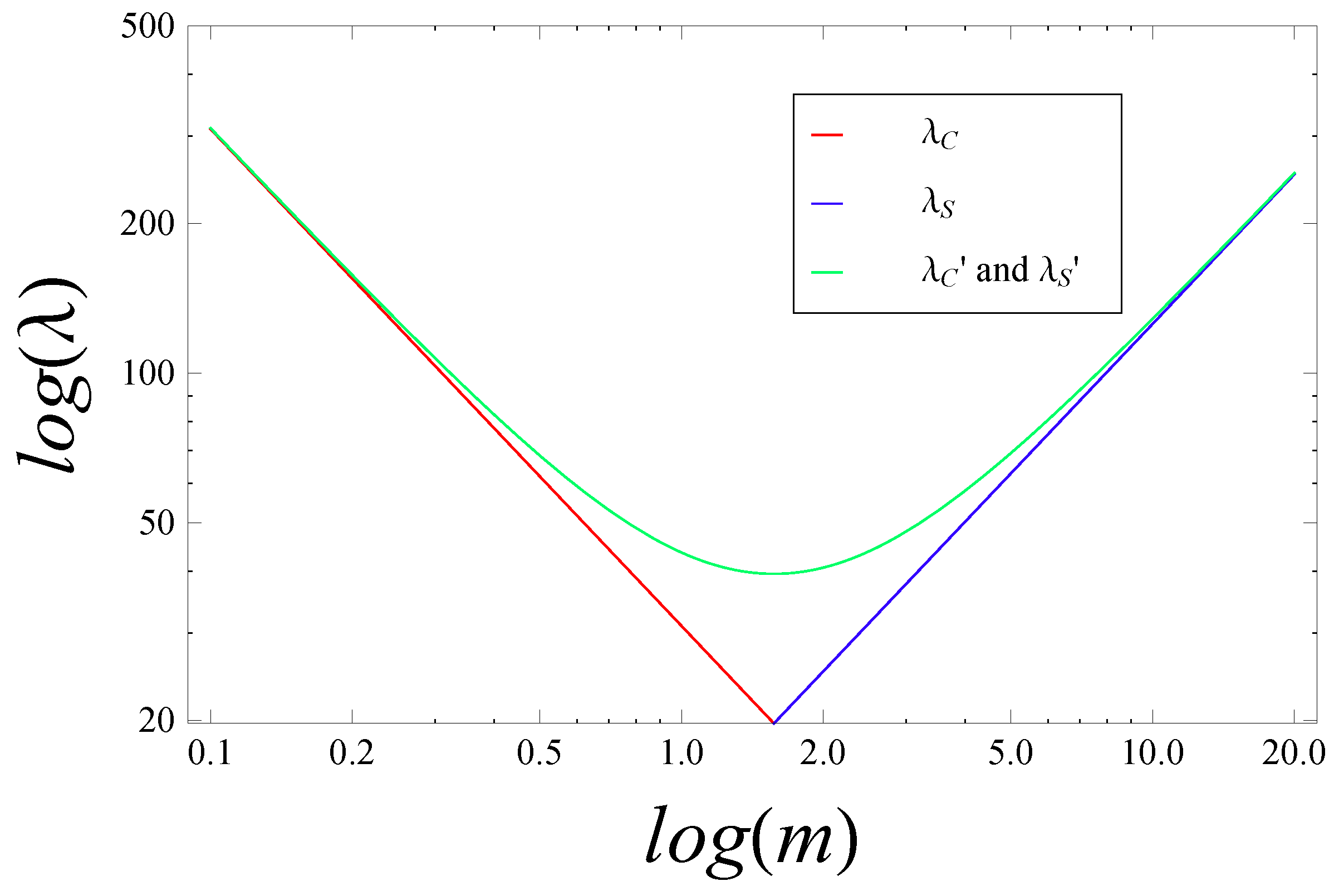
Figure 1 shows the Compton and Schwarzschild lines—here denoted
and
for notational consistency—as asymptotes in the
and
regimes, respectively. The line
represents a possible interpolation between the two regions, in which
and
are unified into a single curve. Since the Compton wavelength may also be “derived” from the HUP in canonical QM by applying the semi-Newtonian approximation, as discussed in
Section 3.4, a unification of this form is known as the black hole uncertainty principle (BHUP) correspondence [
25,
26], as well as the Comtpon-Schwarzschild correspondence [
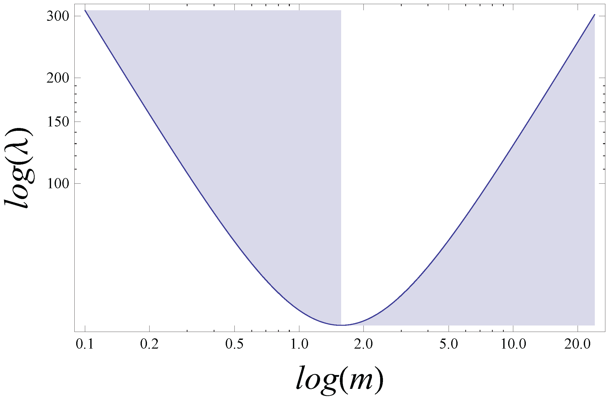
1]. Crucially, we again note that any would-be unified description of particles and black holes must account for the change in the physical nature of the radius
at
, from minimum to maximum spatial extent of the wave packet. This is depicted visually in
Figure 2. In the language of semi-Newtonian QM, the shaded region on the left-hand side of
Figure 2 is associated with the “≥” inequality from the HUP. It is therefore reasonable to expect that the shaded region on the right should be associated with the inequality “≤” in a modified uncertainty relation, giving rise to a different kind of positional uncertainty for black holes. The minimum of the curve
is then associated with equality “=” in which the modified Compton and Schwarzschild radii are equal. This state is unique, with
. (Both
Figure 1 and
Figure 2 are taken from [
1].)
Finally, we note that, in the semi-Newtonian picture, the existence of a minimum radius for the wave packet for implies a UV cut-off for in the usual Fourier expansion of . Likewise, the existence of a maximum radius for implies an IR cut-off in for the wave functions black holes. (That these cut-offs are not fundamental, but instead mark the point at which the semi-Newtonian approximation breaks down, and relativistic effects must be more fully accounted for, need not concern us.) Therefore, if a unified description can be based on a modified quantum dispersion relation, we expect such limits to arise naturally from the relations themselves.
4.1. De Broglie Relations for Black Holes—The Limit
An arbitrary generalization of the usual (one-dimensional) de Broglie relations may be written as
where
and
are arbitrary functions of the angular frequency and wave number, respectively. (For the sake of simplicity, we restrict ourselves to one-dimension, which may also be interpreted as an analysis of spherically symmetric systems.) Let us now suppose that, in the limit
, the generalized de Broglie relations (4.3) take the form
where
is a dimensionless constant. Combining (2.2) (with
) and (4.4), gives the dispersion relation
Assuming that the momentum operator eigenfunctions take the usual form (2.6), the EOM for the quantum state is of Schrödinger type:
which corresponds to modified Hamilton and momentum operators,
and
. The differential part of
takes the standard form, but the multiplying factor differs from the canonical one; the first corresponds to the functional form of the dispersion relation, while the second sets the phenomenologically important length scale for the
regime. We note that this is proportional to
m and is of the same order of magnitude as
, whereas the canonical de Broglie relations yield a natural length scale proportional to
, of the order of
. Assuming that the position operator may be defined as usual, we have
so that the commutator is
The proposed asymptotic form of the extended de Broglie relations (4.4) disturbs the mathematical structure of canonical QM only so far as the momentum operator is multiplied by a constant factor. This modifies the Hamiltonian and momentum operators (and functions of these), together with the commutation relations, but does not affect the underlying Hilbert space structure of the theory. Postulate 4 is changed, but only trivially [
7]. The underlying mathematical formalism is the same as in canonical QM, so that the new theory is well defined in the limit
.
The physical motivation for suggesting the asymptotic form (4.4) is the natural emergence of the Schwarzschild radius as a phenomenologically significant length scale. The modified uncertainty relation gives
For
, we use (2.18), together with the semi-Newtonian approximation, to make the identifications (2.23). By contrast, using (4.9), together with the semi-Newtonian approximation for
, gives
Substituting (4.10) into (4.9), and ignoring numerical factors of order unity, gives , in accordance with our original assumption about the validity of Equation (4.9) in this range. Thus, the identifications (4.10) are consistent with the assumption .
4.2. De Broglie Relations for All Energies
We now propose a physically viable Ansatz for the theory of extended de Broglie relations, which is able to provide a unified description of particles and back holes in the semi-Newtonian approximation. This is intended as a toy model, since deviations from canonical QM behaviour due to gravitational effects have yet to be detected experimentally [
18,
19], and current observations offer no clue regarding the precise mathematical form of the quantum dispersion relation close to the Planck point. In principle, any curve
that asymptotes to both
and
in the appropriate regimes remains phenomenologically viable at the present time.
In this section, we show that, for de Broglie relations that hold for all energies, and take appropriate asymptotic forms for
and
, the quantum EOM is
not, in general, of Schrödinger type. Deviations from Schrödinger-type evolution are most pronounced for
, though the EOM simplify to (2.4) and (4.6) in the small and large mass limits, respectively. Nonetheless, both unitarity and the Hilbert space structure of the canonical theory are preserved throughout the entire mass range. Once again, only Postulate 4 of [
7] must be amended, this time less trivially, while the mathematical structure embodied in Postulates 1, 2 and 3 is unchanged.
The “simplest” form of the functions
and
in Equation (4.3), able to satisfy the physical requirements outlined in
Section 3.4, are:
Though “simplicity” remains a subjective judgement, here we take it to mean that the new functions contain only terms in ω and or k and , in the limit, reflecting the symmetry of the diagram, with only the minimum number of additional free parameters—in this case, the single numerical constant . We note that the continuity of E, p, and , at , , implies . However, since we require continuity of all physical observables at , and β must be fixed to ensure this, we leave it as a free parameter for now.
For
, combining Equations (4.11) and (4.12) with (2.3), gives
which reduces to
for
and
, as required. In general, however, (4.13) may be solved to give
two solution branches,
The reality of both branches requires
and the inequality is saturated for
The reality of these limits then implies
The inequality (4.15) is satisfied for two
disjoint ranges:
Defining
, the lower limit on the value of the wavenumber
corresponds to an upper limit on the wavelength
while the upper limit
corresponds to a lower limit
, so that (4.18) is equivalent to
For
, Equation (4.16) can be expanded to first order, giving
where
, which is equivalent to
We note that the first range of wavelengths given by Equations (4.18) and (4.19) is compatible with the existence of an “outer” radius, which acts as a minimum obervable width for the particle, whereas the second range is compatible with the existence of an “inner" radius, within which sub-Planckian de Broglie modes become trapped, but which remains unobservable. Though it is unclear whether this range is physically meaningful, we note that, formally extending the diagram to implies and for . In this region, acts like an (inner) unobservable radius, which is disjoint from the (outer) observable radius, .
Interestingly, since
, Equation (4.21) gives rise to a minimum length uncertainty relation (MLUR) closely resembling the one originally derived, using heuristic arguments, by Salecker and Wigner [
27] (see also [
28] for recent developments) and later considered by Ng and Vam Dam [
29]:
, where
d is the distance “probed” using a QM measuring device [
30]. For
, the predictions of the extended de Broglie theory coincide with this relation. However, note that, here, we use the notation
, rather than
, to indicate that the “uncertainty” obtained in [
27] differs from the canonical definition given in Equation (2.16). In summary, for
, the extended de Broglie theory implies
and
, where
and
differ as described in [
27,
28,
29,
30].
For
, the counterparts of Equations (4.13)–(4.16) may be obtained by performing the substitution
and the reality conditions on
yield
Again, two discontinuous wavelength ranges are permitted, according to Equation (4.19), but the new limits are given by
These are equivalent to those given in Equation (4.21) under the interchange , up to numerical factors of order unity. This is compatible with the existence of an observable outer radius and an unobservable inner radius .
From Equations (4.17) and (4.23), we see that
is required to ensure the continuity of physical quantities at close to the Planck point. We then have
where
is defined in Equation (4.23), giving
,
and
for
. The continuity of
at
and
at
is ensured and the reality conditions justify our initial assumptions about the division between
and
. Note that the original, approximate, conditions given in Equation (4.11) have now been replaced by the more precise expressions
and
in Equation (4.25).
The solutions obtained above exhibit various dualities: Each branch of the quantum dispersion relation for particles (now defined as spherically symmetric objects with rest masses
) maps to its equivalent for black holes (with rest masses
), under
This is equivalent to a reflection about the line
in the log-log plot of the
plane, at fixed
k. For fixed
m, the self-duality
maps the upper and lower branches of the solution
into one another in the
plane, and
transforms the upper and lower limits on the wave number into one another.
Using the standard definitions of
and
, Equation (4.27) also induces the transformation
, which is equivalent to
. However, since
gives the order of magnitude length scale at which pair production rates become significant, the exact numerical factor used to define it is to some degree arbitrary, whereas the definition of
comes from an exact solution of the EFEs. We are therefore free to redefine
, such that
The new definition gives
so that the duality transformation (4.27) induces
The new definition (4.30) also ensures
at
, so that we may directly associate the divide between
and
in Equations (4.25) and (4.26) with the transition between particles and black holes. For either definition, (2.21) or (4.30), the equivalents of Equations (4.13) and (4.16) for the black hole regime may be obtained (up to factors of order unity multiplying the relevant terms), via the substitution
. The asymptotic regimes of
are then given by
where we choose
for
and
for
. For weakly gravitating particles,
and
, whereas, for black holes,
and
. Both give
.
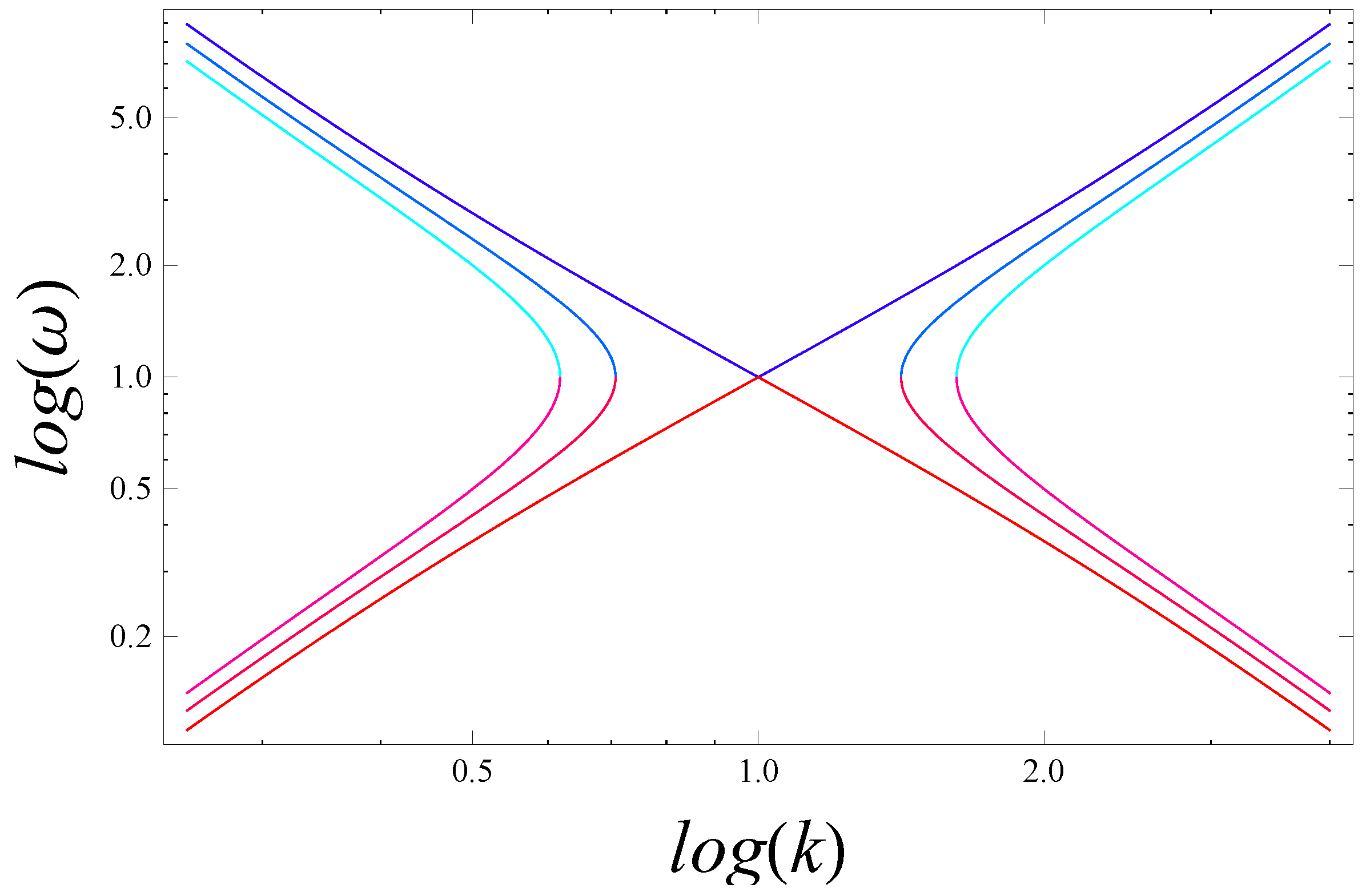
To summarize: Formally, there exist two inequivalent dispersion relations, in each mass range and , corresponding to the separate branches , though the physical interpretation of the branch is unclear, as this corresponds to de Broglie waves with sub-Planckian wavelengths. The super-Planckian branch depends on both k and m, as in canonical QM, but, in the modified theory, there exist limiting values of k, which are also functions of the rest mass. This may be contrasted with the canonical non-relativistic theory, in which all modes may contribute, with some nonzero amplitude, to a given wave packet expansion.
All four solution branches,
for both
and
, are plotted in
Figure 3. However, due to the duality (4.27), we have that
, and the curves corresponding to particles with
are overlaid by the curves corresponding to black holes with masses
. Each curve in the first set, labelled by the mass
m, is overlaid by a curve in the second set, labelled by
, and each quadrant contains
both “particle” and “black hole” solutions. The lower-left, lower-right, upper-left and upper-right quadrants corresponds to the four independent regimes,
,
;
,
;
,
and
,
, respectively. Therefore, only the lower left-hand quadrant is
definitely physical. It describes both quantum particles and quantum black holes with super-Planckian radii. The canonical QM dispersion relation,
, corresponds to the asymptotic regime in the bottom left-hand corner of the diagram.
If the upper half-plane of
Figure 3. is regarded as physical, the upper right-hand quadrant gives the dispersion relation for “sub-Planckian” black holes—that is, black holes with
,
, conjectured to exist in LQG [
31]—or, equivalently, the dispersion relation for “sub-Planckian” particles—that is, particles with
,
. If the latter exist, they may correspond to the point-like matter distributions at the centre of normal (super-Planckian) black holes, thereby preventing the formation of classical singularities. The upper left-hand and lower right-hand quadrants correspond to mixed regimes, where objects are associated with either sub-Planckian time periods and super-Planckian wavelengths, or vice-versa. We note that all four solution branches “touch” in the critical case,
,
,
, which corresponds to a
unique quantum state in the semi-Newtonian picture. The limits
are shown in
Figure 4. (Both
Figure 3 and
Figure 4 are taken from [
1].)
6. Implications for the Hawking Temperature
The Hawking temperature [
33,
34] for black holes may also be obtained heuristically in the semi-Newtonian approximation of canonical QM. Assuming an upper limit for
, associated with the Schwarzschild radius, we obtain a corresponding lower limit on
via the HUP (2.18), giving
may be identified with the momentum uncertainty of a particle emitted during Hawking radiation [
25,
26], and the associated temperature
is defined via
where
is the Planck temperature and
χ is a constant. Agreement with the Hawking temperature requires
, so that
In this scenario, we note that, since is associated with a lower limit on the momentum uncertainty, it represents the minimum temperature that can be associated with the mass m of the black hole. In other words, were an observer to localise m on some scale , for example, by crossing the event horizon, we would expect the temperature associated with m, in their frame, to be greater than .
As shown in
Section 2.2, we may also obtain the standard expression for the Compton wavelength (up to numerical factors of order unity) by associating this with the lower limit on the size of the wave packet
. The corresponding upper limit on the momentum uncertainty
is associated with the particle’s rest mass (2.23). This defines the Compton line on the
diagram, and the numerical factor may be chosen to ensure that the intersect with the Schwarzschild line occurs at
(4.30). This allows us to associate the two halves of the diagram with the extended de Broglie relations for particles and black holes, respectively, given in Equations (4.25) and (4.26).
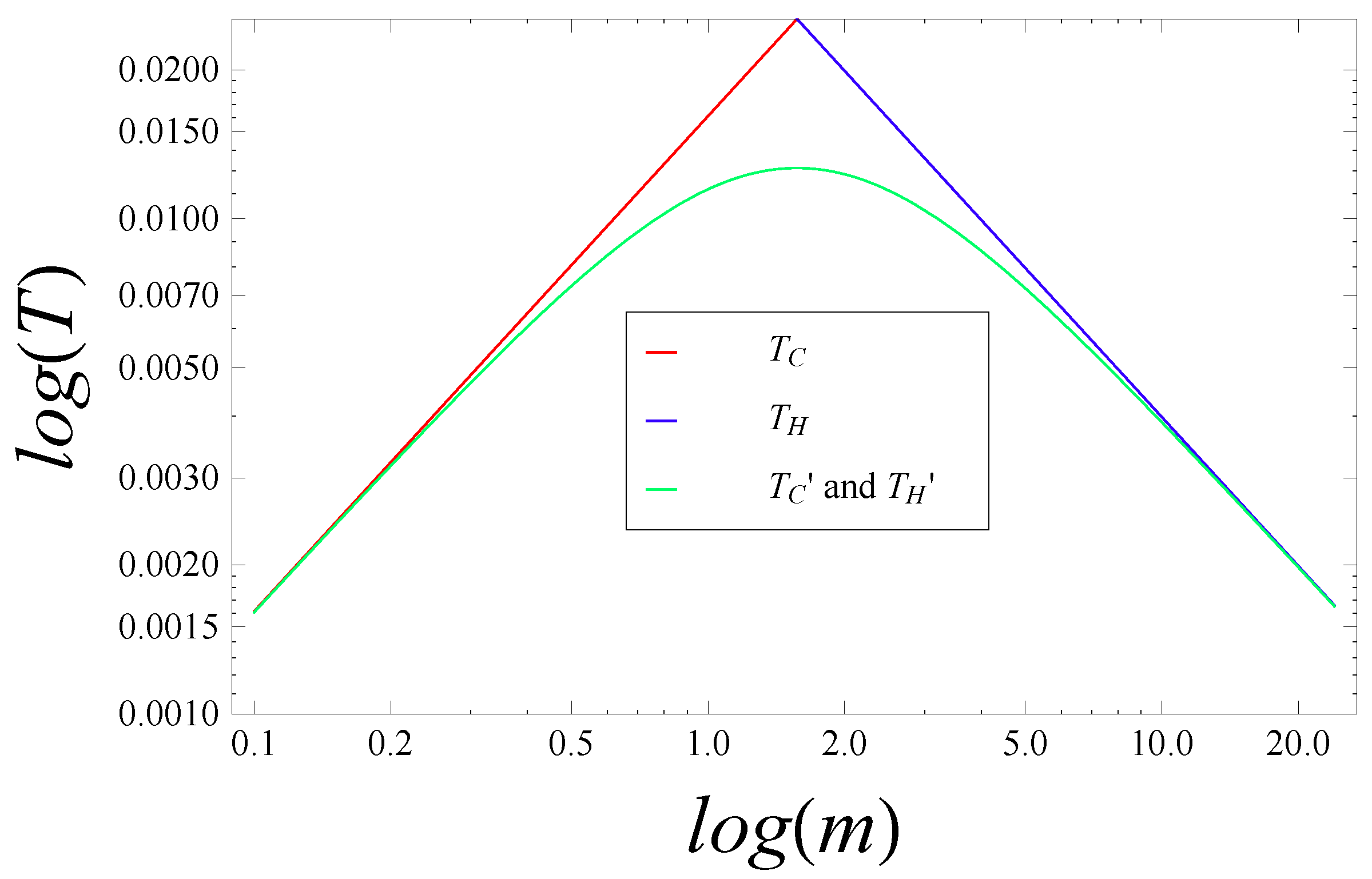
We then define the “Compton temperature” as
where setting
ensures that
at
. This may also be regarded as the natural temperature associated with the rest mass of the particle. By our previous logic, since
is associated with the upper limit on the momentum uncertainty, it represents the
maximum temperature that can be associated with the particle mass
m. This matches our intuition, since particles with real temperatures
, corresponding to wave packets with
, have sufficient kinetic energy to pair produce. Additional increases in the total energy of the system then result in pair production rather than increased temperature. Conversely, wave packets with
are naturally associated with temperatures
, which correspond to kinetic energy uncertainties
.
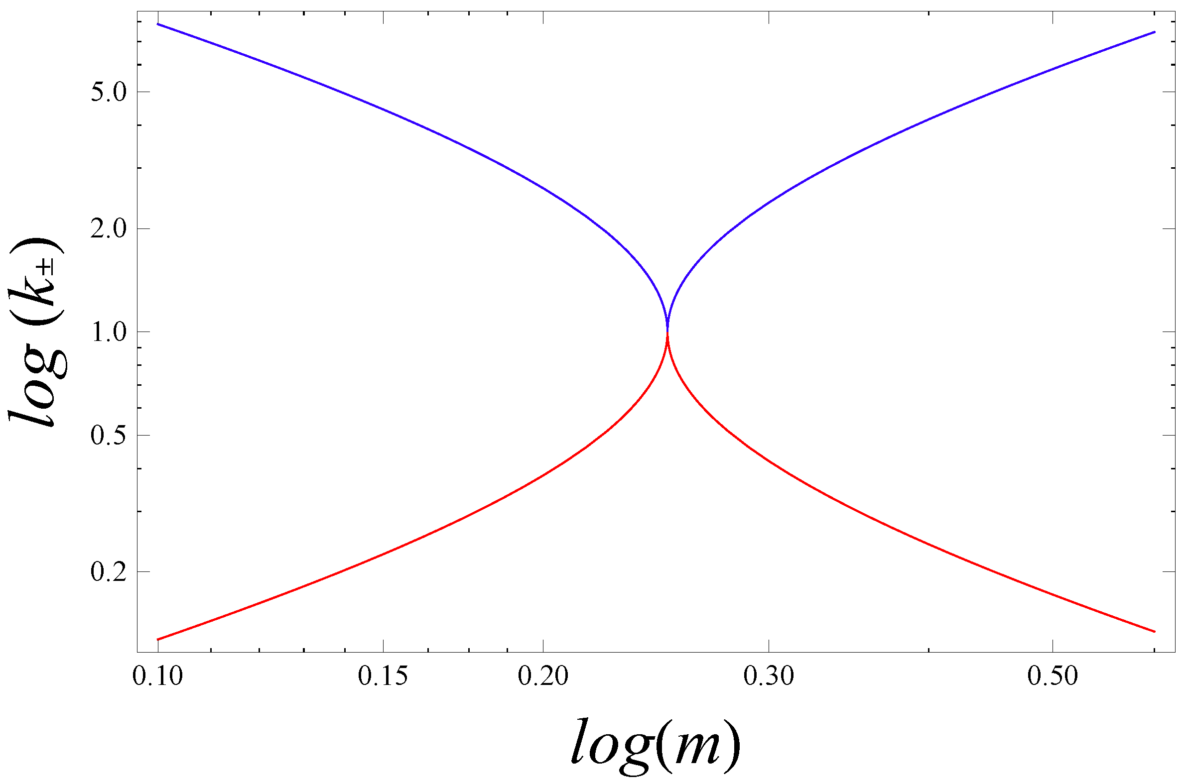
and
are plotted as red and blue lines, respectively, in
Figure 5, which is also taken from [
1]. The green curve
represents a smooth interpolation between the two, which is associated with a unified Compton-Schwarzschild line,
, via
, by analogy with the semi-Newtonian “derivations” of
and
in the asymptotic regions, given above. Just as the physical nature of the radius changes at the critical mass,
, as illustrated explicitly in
Figure 2, so does the physical nature of the temperature. The left-hand and right-hand halves of the green curve in
Figure 5 may be associated with upper and lower limits on
T, respectively, so that the
diagram analogue of
Figure 2 would appear inverted, with shaded and unshaded regions interchanged.
7. Unification of Black Holes and Fundamental Particles from GUP Phenomenology and Its Relation to Extended de Broglie Relations
As discussed in
Section 2.2, substituting the commutator
into the general uncertainty principle (2.16) yields the famous Heisenberg uncertainty principle (HUP)
, which arises as a fundamental consequence of the Hilbert space structure of canonical QM. Although
and
do
not refer to any unavoidable “noise” , “error” or “disturbance” introduced to the system by the act of measurement, it is well known that one can understand this result
heuristically as reflecting the momentum transferred to the particle by a probing photon [
3]. Hence, in order to distinguish between quantities representing genuine noise, induced by the measurement process, and the standard deviations of repeated
perfect, projective, Von Neumann-type measurements, which do not disturb the state
prior to wave function collapse [
7], we use the notation
for the former and
for the latter. (Strictly speaking, any disturbance to the state of the system caused by an act of measurement may also be
-dependent, but we adopt Heisenberg’s original notation, in which the state-dependent nature of the disturbance is not explicit.) In this notation, the formulation of the standard uncertainty principle based on the “Heisenberg microscope” thought experiment may be written as
We note that such a statement must be viewed as a postulate with no rigorous foundation in the underlying mathematical structure of quantum theory. Indeed, as a postulate, it has recently shown to be manifestly false, both theoretically [
35,
36] and experimentally [
37,
38,
39,
40]. However, the heuristic “derivation” of Equation (7.1) may be found in many older texts, alongside the more rigorous derivation of Equation (2.16) from basic mathematical principles. Unfortunately, it is not always made clear that the quantities involved in each expression are different, as clarified by the recent pioneering work of Ozawa [
35,
36]. An excellent discussion regarding the various possible meanings and (often confused) interpretations of symbols like “
” is given in [
41].
The clarifications given above are of key importance when discussing quantum phenomenology based on the Generalised Uncertainty Principle (GUP). This term refers, generically, to
any extension of the the standard HUP (7.1), whether based on fundamental modifications of the mathematical formalism of canonical QM, or simply on heuristic results. It must not be confused with the term “general uncertainty principle” used to describe Equation (2.16), though the terminology adopted in different parts of the literature is confusing [
7].
Many GUP proposals are motivated by attempts to incorporate gravitational effects into existing interpretations of quantum uncertainty. Many also give rise to a minimum length, interpreted as a quantum gravitational effect, and are known as minimum length uncertainty relations (MLURs). (For recent reviews of GUP phenomenology, see [
42,
43]; for reviews of minimum length scenarios in quantum gravity, see [
30,
44].) One of the earliest and most interesting examples of a quantum gravity inspired GUP was proposed by Adler and Santiago [
45],
where
α is a constant of order
. This is based on an extension of the Heisenberg microscope thought experiment, incorporating the effect of the gravitational interaction between the particle and the photon probe, which gives rise to the additional term on the right-hand side. A GUP of this form was originally proposed in the context of string theory [
46], as it implies the existence of a minimum length,
, which may be identified with the fundamental string scale.
From (7.2), it is clear that using the standard identification for the momentum uncertainty
implies
, where
represents a modified Compton wavelength of the form
Thus, for
, the first (Compton) term dominates, whereas, for
, the second (Schwarzschild) term gives the leading order contribution to the total uncertainty. In the this way, a GUP of the form (7.2) may enable a unified description of fundamental particles and black holes based on a modified quantum theory. A GUP-based unification of this this kind, suggested in [
25], is termed the black hole uncertainty principle (BHUP) correspondence. However, several theoretical and conceptual issues arise in the context of such a proposal, which we now address.
First, if we wish to give rigorous mathematical definitions of the terms
and
appearing in Equation (7.2) (i.e., to “promote” them to quantities analogous to
and
, which follow directly from the mathematical formalism of the underlying quantum theory (2.16)), it is clear that we must modify either the Hilbert space structure of canonical QM and/or the commutator
. The former is highly non-trivial, while the latter is equivalent to leaving the state space structure unchanged but modifying the dispersion relations and the EOM for the state vector. This, in turn, may be achieved in several different ways: (i) by maintaining the standard de Broglie relations but modifying the classical energy-momentum relation; (ii) by maintaining the classical energy-momentum relation but modifying the de Broglie relations; and (iii) by modifying both. One approach, based on (ii), gives rise to the modified commutator [
47]
which corresponds to the individual operators
Substituting (7.4) into (2.16) and setting
, so that
, yields a GUP of the form
which is obviously equivalently to (7.2), up to numerical factors of order unity, but which may be derived from first principles. Crucially, the approximation
is valid for spherically symmetric systems, in which it is also reasonable to make the identification
. (In fact, it may be argued that identifying the momentum uncertainty with the rest mass is valid
only in the rest frame of the system, under conditions of spherical symmetry.) Hence, the modified commutator (7.4) is
potentially capable of yielding a unified Compton-Schwarzschild line of the form (7.3) under the identification
, but, for reasons we now address, such an identification is not possible for arbitrary
m.
In [
47], the modified dispersion relations giving rise to Equations (7.4) AND (7.6) are
where the approximations on the right-hand sides of Equations (7.7) are valid for
and
, respectively. If these hold for every de Broglie mode in a single spherically symmetric wave packet, then
. Hence, this identification is incapable of providing a unified description of particles and black holes, as it does not allow for the extension of the modified Compton wavelength
(7.3) into the right-hand side of the
diagram.
However, other considerations suggest an alternative identification between
and the rest mass of a spherically symmetric system for
. Consider a black hole decaying via Hawking radiation: The average magnitude of the momentum of a particle emitted from a black hole of mass
is
, where
is the effective particle mass (even if the particle is a photon). Therefore,
is the total momentum uncertainty; this may also be seen by associating the positional uncertainty of the emitted particle with the black hole radius,
, in the standard HUP, or in the leading order term of the GUP (7.2) for particles with
. Since momentum conservation implies that the recoil of the black hole, due to a
single emission, must be equal in magnitude (but opposite in sign) to the momentum of the outgoing particle, it follows that
. Thus, for general spherically symmetric systems of mass
m – subject to the HUP or a GUP of the form (7.2)—we may associate
An interesting feature of the GUP proposed by Adler and Santiago (7.2) is that it is invariant under the transformation , so that the change in how is associated with the rest mass of the system, occurring at , still enables the construction of a unified Compton-Schwarzschild line of the form (7.3).
We also note that the modified commutator and dispersion relations proposed in [
47] do not alter the fundamental Newtonian nature of space and time (subject to the cosmic speed limit
), since they leave the fundamental commutator between the
and
operators unchanged,
where
What has changed is, instead, is the the intrinsic relation between
p and
k, i.e., the functional form of
. Thus, in this case, the generators of infitesimal translations in the Gallilean symmetry group may still be identified with the
operators; translation invariance gives rise to conserved Noether charges for
classical systems, the components of the classical momentum
,
and to a set of nontrivial commutators (7.9) for quantum systems. However, the hermitian operators
are no longer directly proportional to the de Broglie wave number operators
, due to the more complex form of the modified de Broglie relations (7.9). As with the extended de Broglie relations presented in
Section 4,
Section 5 and
Section 6, these remain the essence of the non-trivial modifications to the quantum sector. (Similar arguments apply regarding time translational symmetry, the frequency operator
, and the classical energy
E, though subject to the caveat that time
t is parameter,
not an operator, in both canonical QM and the modified theories presented here.)
Hence, considering the GUP, together with momentum conservation arguments that give rise to the approximate identifications (7.8) in the two mass regimes, is phenomenologically equivalent to using the HUP together with the associations
which are assumed to be valid for
all m. This makes sense, intuitively, since it relates the positional and momentum uncertainty of quantum-gravitational system to the ADM mass [
31,
48]. We also note that Equation (7.11) gives rise to a unified Compton-Schwarzschild line that is (at least)
qualitatively similar to the effective mass-dependence of
, introduced via the extended de Broglie theory given in
Section 4,
Section 5 and
Section 6. In the latter, however, the rest mass is directly associated with the minimum uncertainty of a
modified momentum operator
(4.10). The arguments presented here suggest that this
cannot be identified with the physical recoil of the black hole during the Hawking emission of a fundamental particle.
Another crucial difference between the two approaches is that the modified de Broglie relations proposed in [
47], Equations (7.7), predict an
almost unique quantum state for
all black holes, since
for
and
for
. This is a direct result of the fundamental asymmetry between the form of the relations (7.7) for
and
. By contrast, the extended de Broglie theory presented in
Section 4,
Section 5 and
Section 6 explicitly incorporates the symmetry between fundamental particles and black holes present in the
diagram, via the extensions of the relations themselves. In this scenario, the unique quantum state
corresponds to the unique physical state for which Schwarzschild radius is equal to the Compton wavelength.
A related point concerns the fact that
all forms of modified quantum mechanics proposed thus far in the literature—be they based directly on GUP phenomenology or on modified de Broglie relations—give rise to uncertainty relations of the form
, even when these are extended to systems with super-Planckian rest mass. This is the mathematical expression of the assumption that the radius of a black hole is, in some sense, physically equivalent to the radius of fundamental particle, i.e., that it may be considered as a minimum, rather than as a maximum limit on rest mass localisation. Were
ψ to represent (in some limit) the wave function associated with the mass in the interior of a black hole, it may be argued that a modified quantum theory giving rise to a positional uncertainty of the form
is required. It would be interesting to consider how such a theory could be reconciled with the “horizon wave function” model, proposed by Casadio et al. (see, for example [
49,
50,
51,
52]), as even an effective wave function model of a black hole may require
both components.
8. Conclusions
We have shown that, by taking the semi-Newtonian approximation, in which space and time remain absolute but a cosmic speed limit is imposed “by hand”, we can recover essential phenomenological features of both relativistic quantum theory and relativistic gravity from their non-relativistic counterparts. Applying this approximation to the basic mathematical structure of canonical QM yields the formula for the Compton wavelength, via the uncertainty principle, while applying it to Newtonian gravity yields the Schwarzschild radius, via the formula for the escape velocity. On a plot of mass versus radius, these lines meet at the Planck point, suggesting that the final theory of quantum gravity should yield a unified description of fundamental particles and black holes. In the absence of such a theory, we propose a naïve unification, based on recognition of the fact that both sets of objects may be adequately described in the semi-Newtonian regime.
Since the canonical QM dispersion relations break down for Planck mass objects, our new theory is based on modified de Broglie relations, which, when substituted into the classical energy-momentum relation, yield quantum dispersion relations that hold for systems of arbitrary mass. These, in turn, give rise to modified EOM, Hamiltonian, momentum and time-evolution operators, in both the particle and black hole sectors. In each sector, the time-evolution is non-canonical, but unitary, and the particle evolution reduces to canonical form in the asymptotic limit. The new dispersion relations depend on all three fundamental constants, G, c and ℏ, and their chosen form gives rise to a new mass-dependence in the phenomenologically significant length scale of the theory. This reduces to the Compton radius for extreme low-mass objects, but corresponds to the Schwarzschild radius in the opposite extreme. We therefore interpret the additional terms in the modified dispersion relations as representing the self-gravity of the quantum wave packet in the semi-Newtonian picture.
In addition, our work suggests a natural definition for the “Compton temperature” of a fundamental particle. This bears the same relation to the Compton wavelength as does the Hawking temperature of a black hole to its Schwarzschild radius, and may be interpreted as the temperature associated with the particle’s rest mass. In the extended de Broglie theory, the two lines, plotted as functions of mass on a log-log plot, define asymptotes to a unified temperature curve, which interpolates between the particle and black hole regions. In this formulation, a Planck mass object is represented by a unique quantum state, whose de Broglie wavelength, Compton wavelength and Schwarzschild radius are equal to the Planck length, and whose temperature is equal to the Planck temperature.
To summarize: The pedagogical discussions in
Section 2 and
Section 3 aim to clarify the physical assumptions and mathematical foundations on which the extended de Broglie theory is based, while
Section 4,
Section 5 and
Section 6 consider its detailed predictions. The discussion in
Section 7 sets the theory proposed in
Section 4,
Section 5 and
Section 6 in the context of the existing literature on modified quantum theories, which attempt to incorporate gravitational effects. Though we make no claims for the quantitative validity of this theory, originally proposed in [
1], it is hoped that the considerations raised therein, and in the (expanded) discussion presented here, will help stimulate debate on the important open questions in black hole physics: “Which quantum theory must be reconciled with gravity? (And what does it mean for black holes?)”.

