On the Effect of the Cosmological Expansion on the Gravitational Lensing by a Point Mass

Abstract

We analyse the effect of the cosmological expansion on the deflection of light caused by a point mass, adopting the McVittie metric as the geometrical description of a point-like lens embedded in an expanding universe. In the case of a generic, non-constant Hubble parameter, H, we derive and approximately solve the null geodesic equations, finding an expression for the bending angle δ, which we expand in powers of the mass-to-closest approach distance ratio and of the impact parameter-to-lens distance ratio. It turns out that the leading order of the aforementioned expansion is the same as the one calculated for the Schwarzschild metric and that cosmological corrections contribute to δ only at sub-dominant orders. We explicitly calculate these cosmological corrections for the case of the H constant and find that they provide a correction of order 10⁻¹¹ on the lens mass estimate.

1. Introduction

The effect of the cosmological constant Λ (and thus, by extension, of cosmology) on the bending of light is an issue which has raised interest since a pioneering work by Rindler and Ishak in 2007 [1]. The common intuition is that Λ cannot have any local effect on the deflection of light because it is homogeneously distributed in the universe, thus not forming lumps which may act as lenses. Moreover, General Relativity (GR) is assumed as the fundamental theory of gravity, and the Kottler metric is considered [2] (We use throughout this paper $G=c=1$ units):

$$d{s}^2=f(r)d{t}^2-f^{-1}(r)d{r}^2-r^{2}d{\Omega }^2,$$

(1)

where $d{\Omega }^2=d{\theta }^2+{sin}^2\theta d{\varphi }^2$ and:

$$f(r)\equiv 1-\frac{2M}{r}-\frac{\Lambda r^2}{3},$$

(2)

as the description of a point mass M embedded in a de Sitter space. It turns out that Λ does not appear in the null geodesic trajectory equation, cf. e.g., Equation (17) of Ref. [3]. Indeed:

$$\frac{d^{2}u}{d{\varphi }^2}+u=3M{u}^2,$$

(3)

where $u=1/r$ is the inverse of the radial distance from the lens. Therefore, one may conclude that Λ does not affect the bending of light, which is then entirely due to the presence of the point mass M.

On the other hand, in Ref. [1], the authors point out that the bending angle cannot be calculated as the angle between the asymptotic directions of the light ray, since these do not exist. Indeed, from Equation (2), one sees that $r\le \sqrt{3/\Lambda }$, i.e., a cosmological horizon exists. In other words, the effect of Λ enters into the boundary conditions that we choose when solving Equation (3).

Thus, the authors of Ref. [1] find that Λ enters the definition of the deflection angle in the following way (cf. their Equation (17)):

$${\psi }_0\approx \frac{2M}{R}\left(1-\frac{2M^2}{R^2}-\frac{\Lambda R^4}{24M^2}\right),$$

(4)

where R is the closest approach distance. Twice ${\psi }_0$ is the deflection angle. Therefore, one identifies the well-known Schwarzschild contribution $4M/R$, weighed by Λ, which tends to thwart the deflection.

After Ref. [1], many authors confirmed with their calculations that Λ does enter the formula for the deflection angle, although sometimes in a way different from the one in Equation (4). See e.g., Refs. [4,5,6,7,8,9,10,11,12].

On the other hand, there are a few works that do not agree with the above-mentioned results (see e.g., [13,14,15,16]). The main criticism is that the Hubble flow is not properly taken into account, i.e., the relative motion among source, lens and observer is neglected. In particular, the authors of Ref. [15] argue that the Λ contribution in Equation (4) is cancelled by the aberration effect due to the cosmological relative motion. Another interesting remark made in Ref. [15] is that the contribution of Λ to the deflection angle does not vanish for $M\to 0$ in Equation (4). In this respect, consider also e.g., Equation (25) of Ref. [10]:

$$\delta =\frac{4M}{b}-Mb\left(\frac{1}{r_S^2}+\frac{1}{r_O^2}\right)+\frac{2Mb\Lambda }{3}-\frac{b\Lambda }{6}(r_S+r_O)-\frac{b^3\Lambda }{12}\left(\frac{1}{r_S}+\frac{1}{r_O}\right)+\frac{M{b}^3\Lambda }{6}\left(\frac{1}{r_S^2}+\frac{1}{r_O^2}\right)+\cdots .$$

(5)

Here, b is the impact parameter and $r_S$ and $r_O$ are the radial distances from the lens to the source and to the observer, respectively. Taking the limit $M\to 0$ in the above equation does not imply $\delta \to 0$.

This seems to be odd since we do not expect lensing without a lens. However, this is the result that one obtains when the Hubble flow is not taken into account. Indeed, the author of Ref. [16] constructs “by hand” cosmological observers in the Kottler metric and finds that Λ has no observable effect on the deflection of light.

Therefore, according to the results of Refs. [13,14,15,16], the standard approach to gravitational lensing does not need modifications. For the sake of clarity, the standard approach to gravitational lensing consists of using the result on the deflection angle obtained from the Schwarzschild metric (which models the lens) together with the cosmological angular diameter distances calculated from the Friedmann–Lemaître-Robertson–Walker (FLRW) metric. See e.g., Ref. [17].

In Ref. [18], we also tackled the investigation of whether a cosmological constant might affect the gravitational lensing by adopting the McVittie metric [19] as the description of the lens. The McVittie metric is an exact spherically symmetric solution of Einstein equations in presence of a point mass and a cosmic perfect fluid. See e.g., Refs. [20,21,22,23,24,25,26,27,28] for mathematical investigations of the geometrical properties of McVittie metric. In Ref. [18], we considered a constant Hubble factor, thus the geometry involved is the very Kottler one considered by most of the authors cited in this paper, but written in a different reference frame. Our results corroborate those of Refs. [13,14,15,16].

In the present paper, we generalise the results of Ref. [18] to the case of a generic time-dependent H. See also Ref. [29]. This is necessary in order to make contact with the current standard model of cosmology, the ΛCDM model, in which pressure-less matter prevents H to be a constant. In particular, Friedmann equation for the spatially-flat ΛCDM model reads:

$$\frac{H^2}{H_0^2}={\Omega }_{\mathrm{m}}{a}^{-3}+{\Omega }_{\Lambda },$$

(6)

where $H_0$ is the Hubble constant, a is the scale factor, ${\Omega }_{\mathrm{m}}$ is the present density parameter of pressure-less matter and ${\Omega }_{\Lambda }=1-{\Omega }_{\mathrm{m}}$ is the present density parameter of the cosmological constant. The time-derivative of H can be easily computed as:

$$\frac{\dot{H}}{H_0^2}=-\frac{3}{2}{\Omega }_{\mathrm{m}}{a}^{-3}.$$

(7)

Since ${\Omega }_{\mathrm{m}}\approx 0.3$, one can see that ${\dot{H}}_0$ and $H_0^2$ are of the same order at present time. Moreover, $|\dot{H}|\ge H^2$ for $1+z\ge \sqrt[3]{2{\Omega }_{\Lambda }/{\Omega }_{\mathrm{m}}}$. This gives a redshift $z>1.67$. Many of the observed sources and lenses have redshifts larger than this limit (see e.g., the CASTLES survey, https://www.cfa.harvard.edu/castles/); therefore, the above calculation shows that assuming H constant is a very bad approximation and if one plans to make contact with observation, it is necessary to go beyond the static case of the Kottler metric. The McVittie metric with a generic, non-constant H provides an opportunity to do this.

Very recently, the deflection of light in a cosmological context with a generic $H(t)$ has been considered in Ref. [30]. The main result is the following, cf. Equation (11) of Ref. [30]:

$$\Delta \tilde{\phi }=\frac{4{\tilde{M}}_{\text{MSH}}}{\tilde{R}}-2H^2{\tilde{R}}^2,$$

(8)

where ${\tilde{M}}_{\text{MSH}}$ is the Misner–Sharp–Hernandez mass [31,32] contained in a radius $\tilde{R}=a(t)r$. Hence, it turns out that the effect of cosmology on the gravitational lensing depends on whether one takes into account the total contribution (local plus cosmological) to the mass or just the local one. However, in both cases, ${\tilde{M}}_{\text{MSH}}$ can be decomposed in the local m contribution plus the cosmological one, which is cancelled by the $-2H^2{\tilde{R}}^2$ in the above Equation (8). Thus, it appears that the net result is that the cosmic fluid does not contribute directly to the gravitational lensing.

As a final remark, we must stress that the McVittie metric is an oversimplified model of an actual lens, which has a more complicated structure than that of a point. However, the results of our investigation may shed an important light and give valuable insights for future research that takes into account a more complex structure of the lens. As far as we know, lenses with structures different from a point have been considered only by Ref. [10].

The present paper is structured as follows. In Section 2, we present the McVittie metric and its principal features. In Section 3, we obtain the null geodesic equations and calculate the deflection angle. In Section 4, we focus on the case of a constant H and calculate exactly the subdominant contribution to the deflection angle, estimating a relative correction on the mass determination of about 10⁻¹¹, due to the Hubble flow. In Section 5, we present our conclusions. Throughout the paper, we use $G=c=1$ units.

2. The McVittie Metric

The McVittie metric [19] can be written in the following form:

$$d{s}^2=-{\left(\frac{1-\mu }{1+\mu }\right)}^{2}d{t}^2+{(1+\mu )}^{4}a{(t)}^2(d{\rho }^2+{\rho }^{2}d{\Omega }^2),$$

(9)

where $a(t)$ is the scale factor, $d{\Omega }^2=d{\theta }^2+{sin}^2\theta d{\varphi }^2$ and

$$\mu \equiv \frac{M}{2a(t)\rho },$$

(10)

where M is the mass of the point. One can check that for $a=$ constant, the Schwarzschild metric in isotropic coordinates is recovered, whereas for $M=0$, the FLRW metric is recovered.

When $\mu \ll 1$, the McVittie metric (9) can be approximated by:

$$d{s}^2=-\left(1-4\mu \right)d{t}^2+(1+4\mu )a{(t)}^2(d{\rho }^2+{\rho }^{2}d{\Omega }^2),$$

(11)

i.e., it takes the form of a perturbed FLRW metric in the Newtonian gauge with gravitational potential $2\mu$. Since there is only a single gravitational potential, then no anisotropic pressure is present [17,33].

Since null geodesics are conformally invariant, the scale factor $a(t)$ can be written as a conformal factor in front of Equation (11), replacing the cosmic time with the conformal time. The time dependence of the photon trajectory appears then only in μ which, from Equation (10), represents an effective mass decreasing inversely proportional to the cosmic expansion. We are going to show that most of the deflection takes place at the closest approach distance to the lens. Therefore, we can already estimate that at this moment the effective mass of the lens would be $M/a_L$, where $a_L$ is the scale factor evaluated at the moment of closest approach. Therefore, the bending angle shall be proportional to $M/a_L$, and this is indeed our result from Equation (47).

Note also that the gravitational potential $2\mu =M/(a\rho )$ resembles the Newtonian one but with an effective mass that reduces with time or a gravitational radius that increases with time. On the other hand, we know from cosmological linear perturbation theory that, in the matter-dominated epoch, the gravitational potential is time-independent. Therefore, the McVittie metric cannot offer a realistic model of a gravitational lens.

Calculating the Einstein tensor from the McVittie line element (9), one gets:

$${G^t}_t=3H^2,{G^r}_r={G^{\theta }}_{\theta }={G^{\varphi }}_{\varphi }=3H^2+\frac{2\dot{H}(1+\mu )}{1-\mu },$$

(12)

from which one deduces that the pressure of the cosmological medium has the following form:

$$P=-\frac{1}{8\pi }\left[3H^2+\frac{2\dot{H}(1+\mu )}{1-\mu }\right],$$

(13)

i.e., it is not homogeneous and diverging when $\mu =1$. If $H=$ constant, then there is no divergence and the pressure is also a constant. This is the case of the Schwarzschild–de Sitter space, described by the Kottler metric [2]. When $\dot{H}\ne 0$, far away from the point mass, i.e., for $\mu \ll 1$, one gets the usual result of cosmology:

$$P=-\frac{1}{8\pi }\left(3H^2+2\dot{H}\right)+\mathcal{O}(\mu )=-\rho -\frac{\dot{H}}{4\pi }+\mathcal{O}(\mu ),$$

(14)

i.e., the acceleration equation. Isotropy is preserved since ${G^r}_r={G^{\theta }}_{\theta }={G^{\varphi }}_{\varphi }$, i.e., there is no anisotropic pressure, as we already mentioned.

Following Faraoni [28], but also Park [13], the McVittie metric (9) can be reformulated in terms of the areal radius

$$R=a\rho {(1+\mu )}^2,$$

(15)

and gets the following form:

$$d{s}^2=-\left(1-\frac{2M}{R}-H^2{R}^2\right)d{t}^2+\frac{d{R}^2}{1-\frac{2M}{R}}-\frac{2HR}{\sqrt{1-\frac{2M}{R}}}dtdR+R^{2}d{\Omega }^2.$$

(16)

Changing the time coordinate to

$$F(r,t)dT=dt+\frac{HR}{\sqrt{1-\frac{2M}{R}}(1-\frac{2M}{R}-H^2{R}^2)}dR,$$

(17)

the above line element (16) can be finally cast as

$$\begin{array}{c}\hfill d{s}^2=-\left(1-\frac{2M}{R}-H^2{R}^2\right)F^{2}d{T}^2+\frac{d{R}^2}{1-\frac{2M}{R}-H^2{R}^2}+R^{2}d{\Omega }^2.\end{array}$$

(18)

If H is constant, then F can be set to unity and we recover the Kottler metric. Using Equation (18) and calculating the Misner–Sharp–Hernandez mass [31,32] of a sphere of proper radius R, one finds [28]:

$$m_{\text{MSH}}=M+\frac{H^2{R}^3}{2}=M+\frac{4\pi }{3}\rho R^3,$$

(19)

which contains the time-independent contribution M from the point mass plus the mass of the cosmic fluid contained in the sphere. Therefore, M has indeed the physical meaning of the mass of the point. In the Kottler case, one can also define a Komar integral, or Komar mass, and verify that it is indeed equal to M [34].

3. The Bending of Light in the McVittie Metric

We now revisit the calculation for the bending angle performed in Ref. [18], but take into account a general non-constant Hubble factor $H(t)$. We perform the calculations in two different ways: the one in this section is also used in Ref. [18] and is based on the approach usually adopted to study weak lensing (see e.g., Ref. [33,35]). In this approach, the origin of the coordinate system is occupied by the observer. The second way is the one in which the lens is put at the origin of the coordinate system and it is employed in Appendix A.

We adopt μ as perturbative parameter and work at the first order approximation in μ. The observed angle of a lensed source is of the order of the arc second, which corresponds to ${\theta }_O\approx {10}^{-6}$ radians. See e.g., the CASTLES survey lens database (https://www.cfa.harvard.edu/castles/). At least for Einstein ring systems, the bending angle is of order $\delta \approx {10}^{-6}$, i.e., it is of the same order as the observed deflection angle. However, at the same time, the bending angle is of the same order of μ. Therefore, we draw the conclusion that $\mu \approx {10}^{-6}$ and the truncation error, when working at first order in μ, is $\mathcal{O}({10}^{-12})$.

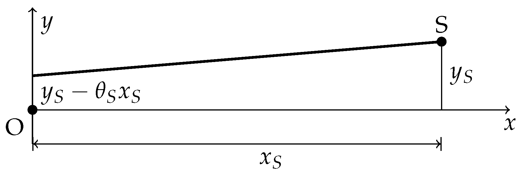
The geometry of the lensing process is depicted in Figure 1. In this scheme, the observer stays at the origin of the spatial coordinate system and x is the comoving coordinate along the observer-lens axis.

The observer has spatial position $(0,0,0)$ and the lens has spatial position $(x_L,0,0)$. The McVittie metric (9) written in Cartesian spatial coordinates is the following:

$$d{s}^2=-{\left(\frac{1-\mu }{1+\mu }\right)}^{2}d{t}^2+{(1+\mu )}^{4}a{(t)}^2{\delta }_{ij}d{x}^{i}d{x}^j.$$

(20)

Note that the spherical symmetry of the McVittie metric implies rotational symmetry about the observer-lens axis. Therefore, we set $z=0$ without losing generality and the source has thus spatial position $(x_S,y_S,0)$.

Since in metric (9) the lens lays at the origin of the coordinate system, we have to perform a translation along the x axis in the Cartesian coordinates of metric (20), so that μ gets the following form:

$$\mu =\frac{M}{2a(t)\sqrt{{(x-x_L)}^2+y^2+z^2}}.$$

(21)

Introducing an affine parameter λ and the four-momentum $P^{\mu }=d{x}^{\mu }/d\lambda$, we can derive from metric (20) the following relation:

$$g_{\mu \nu }{P}^{\mu }{P}^{\nu }=0\Rightarrow P^0=\frac{1+\mu }{1-\mu }p\sim (1+2\mu )p,$$

(22)

where $p^2=g_{ij}{P}^i{P}^j$ is the proper momentum. The above equation represents the usual gravitational redshift experienced by a photon passing through the potential well generated by the point mass. Note that this potential well is not static since μ is time-dependent.

Now, we calculate the geodesic equations for the photon propagating in the McVittie metric (20):

$$\frac{d^2{x}^{\nu }}{d{\lambda }^2}+{\Gamma }_{\alpha \beta }^{\nu }\frac{d{x}^{\alpha }}{d\lambda }\frac{d{x}^{\beta }}{d\lambda }=0.$$

(23)

The geodesic equation for $\nu =0$ has the following form:

$$\frac{d{P}^0}{d\lambda }=2\dot{\mu }{(P^0)}^2+4{\mu }_{,i}{P}^0{P}^i-p^2[H(1+4\mu )+2\dot{\mu }].$$

(24)

Using Equation (22) and the fact that, from Equation (10), $\dot{\mu }=-H\mu$, one finds:

$$p\frac{dp}{dt}=-H{p}^2+2H\mu p^2+4{\mu }_{,i}{P}^{i}p.$$

(25)

The zeroth-order term $H{p}^2$ represents the usual cosmological redshift term. The spatial geodesics equations have the form:

$$\frac{d{P}^i}{d\lambda }=\frac{4{\delta }^{il}{\mu }_{,l}{p}^2}{a^2}-2Hp{P}^i-4P^i{P}^k{\mu }_{,k}.$$

(26)

We now look for an equation for the quantity $dy/dx\equiv tan\theta$, which represents the slope of the line tangent to the photon trajectory. Note that θ is a physical angle because of the isotropic form of metric (20).

Since we can invert $x(\lambda )$ to $\lambda (x)$, being it a monotonic function, we can rewrite Equation (26) for y and change the variable to x:

$$P^x\frac{d}{dx}\left(P^x\frac{dy}{dx}\right)=4{\mu }_{,y}[{(P^x)}^2+{(P^y)}^2]-2Ha(1+2\mu )\sqrt{{(P^x)}^2+{(P^y)}^2}{P}^x\frac{dy}{dx}-4\frac{dx}{dz}{P}^x[P^y{\mu }_{,y}+P^x{\mu }_{,x}],$$

(27)

where we used the fact that

$$p^2=a^2(1+4\mu )[{(P^x)}^2+{(P^y)}^2].$$

(28)

Expanding the left-hand side and using $P^y/P^x=dy/dx$, we obtain:

$$\frac{d^{2}y}{d{x}^2}+\frac{1}{P^x}\frac{d{P}^x}{dx}\frac{dy}{dx}=4{\mu }_{,y}\left[1+{\left(\frac{dy}{dx}\right)}^2\right]-2Ha(1+2\mu )\sqrt{1+{\left(\frac{dy}{dx}\right)}^2}\frac{dy}{dx}-4\frac{dy}{dx}\left(\frac{dy}{dx}{\mu }_{,y}+{\mu }_{,z}\right).$$

(29)

In order to determine the second term on the left-hand side, we use Equation (26) for x:

$$\begin{array}{c}\hfill \frac{1}{P^x}\frac{d{P}^x}{dx}=4{\mu }_{,x}\left[1+{\left(\frac{dy}{dx}\right)}^2\right]-2Ha(1+2\mu )\sqrt{1+{\left(\frac{dy}{dx}\right)}^2}-4\left(\frac{dy}{dx}{\mu }_{,y}+{\mu }_{,z}\right).\end{array}$$

(30)

Combining the two Equations (29) and (30), we finally find:

$$\frac{d^{2}y}{d{x}^2}=4{\mu }_{,y}\left[1+{\left(\frac{dy}{dx}\right)}^2\right]-4{\mu }_{,x}\left[1+{\left(\frac{dy}{dx}\right)}^2\right]\frac{dy}{dx}.$$

(31)

Let’s discuss a little about the spatial derivative of μ. From Equation (21), we get:

$${\mu }_{,y}=-\mu \frac{y}{\sqrt{{(x-x_L)}^2+y^2}},$$

(32)

and

$${\mu }_{,x}=-\mu \frac{(x-x_L)}{\sqrt{{(x-x_L)}^2+y^2}}.$$

(33)

Notice that, when $\mu =0$, Equation (31) becomes:

$$\frac{d^{2}y}{d{x}^2}=0,$$

(34)

i.e., the zeroth-order trajectory is, as expected, a straight line in comoving coordinates.

We now make a second approximation: we assume $dy/dx=tan\theta$ to be small. From the CASTLES survey we know that the observed angle ${\theta }_O$ is of the order of the arc second, which corresponds to ${\theta }_O\approx {10}^{-6}$ radians. The latter is larger that the actual angular position of the source, say ${\theta }_S$, because of the lensing geometry, see e.g., Figure 2. For this reason, we can assume $dy/dx$ to be small along all the trajectory. Since $dy/dx=tan\theta$, then $dy/dx=\theta +{\theta }^3/3+\cdots$. The truncation error is then of order $\mathcal{O}({\theta }^3)\sim {10}^{-18}$.

We consider Equation (31) up to the lowest order term, i.e.,

$$\frac{d^{2}y}{d{x}^2}=4{\mu }_{,y}+\mathcal{O}(\mu \theta ),$$

(35)

where $\mathcal{O}(\mu \theta )\sim {10}^{-12}$. Using Equation (32) for the derivative ${\mu }_{,y}$, the above equation becomes:

$$\frac{d^{2}y}{d{x}^2}=-\frac{2My}{a(x){[{(x-x_L)}^2+y^2]}^{3/2}}.$$

(36)

Note that a is a function of time, but inverting $x(t)$, we can write a as a function of x. For simplicity, we normalise x, y and $2M$ to $x_L$, thus obtaining:

$$\frac{d^{2}Y}{d{X}^2}=-\alpha \frac{Y}{a(X){[{(X-1)}^2+Y^2]}^{3/2}},$$

(37)

where $Y\equiv y/x_L$, $X\equiv x/x_L$ and $\alpha \equiv 2M/x_L$. The above equation was already found in Ref. [18]. Since $dY/dX=tan\theta$ and $tan\theta \sim \theta$, we can cast the above equation in the following form:

$$\frac{d\theta }{dX}=-\alpha \frac{Y}{a(X){[{(X-1)}^2+Y^2]}^{3/2}}.$$

(38)

We define the bending angle as follows:

$$\delta \equiv {\int }_{{\theta }_S}^{{\theta }_O}d\theta =-\alpha {\int }_{X_S}^0\frac{Y(X)dX}{a(X){[{(X-1)}^2+Y{(X)}^2]}^{3/2}},$$

(39)

i.e., as the variation of the slope of the trajectory between the source and the observer.

We shall solve the above equation keeping the first order in α. The order of magnitude of α can be estimated as follows:

$$\alpha \equiv \frac{2M}{x_L}\approx 2M{H}_0/z_L,$$

(40)

where we assumed a small redshift $z_L$. The above approximation becomes an exact result in the case of a constant Hubble parameter (see e.g., (51)).

Therefore, α is proportional to the ratio between the Schwarzschild radius of the lens and the Hubble radius. This is $H_{0}M\sim {10}^{-12}$ for a galaxy of 10¹⁰ M_⊙ and $H_{0}M\sim {10}^{-9}$ for a cluster of 10³ galaxies each of mass 10¹⁰ M_⊙.

We now devote a small paragraph to the zeroth-order solution.

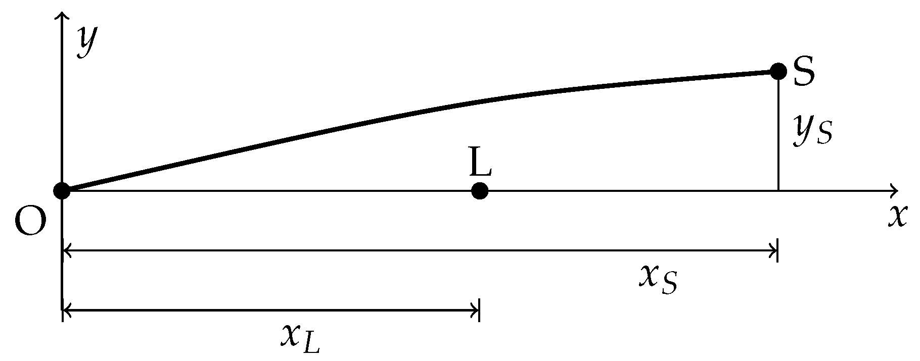
3.1. The Zeroth-Order Solution

The zeroth-order solution (i.e., the one for $\alpha =0$) of Equation (37) is a straight line in comoving coordinates:

$$y={\theta }_S(x-x_S)+y_S,$$

(41)

where ${\theta }_S\ll 1$ is the slope of the trajectory and $(x_S,y_S)$ are the comoving coordinates of the source. See Figure 3.

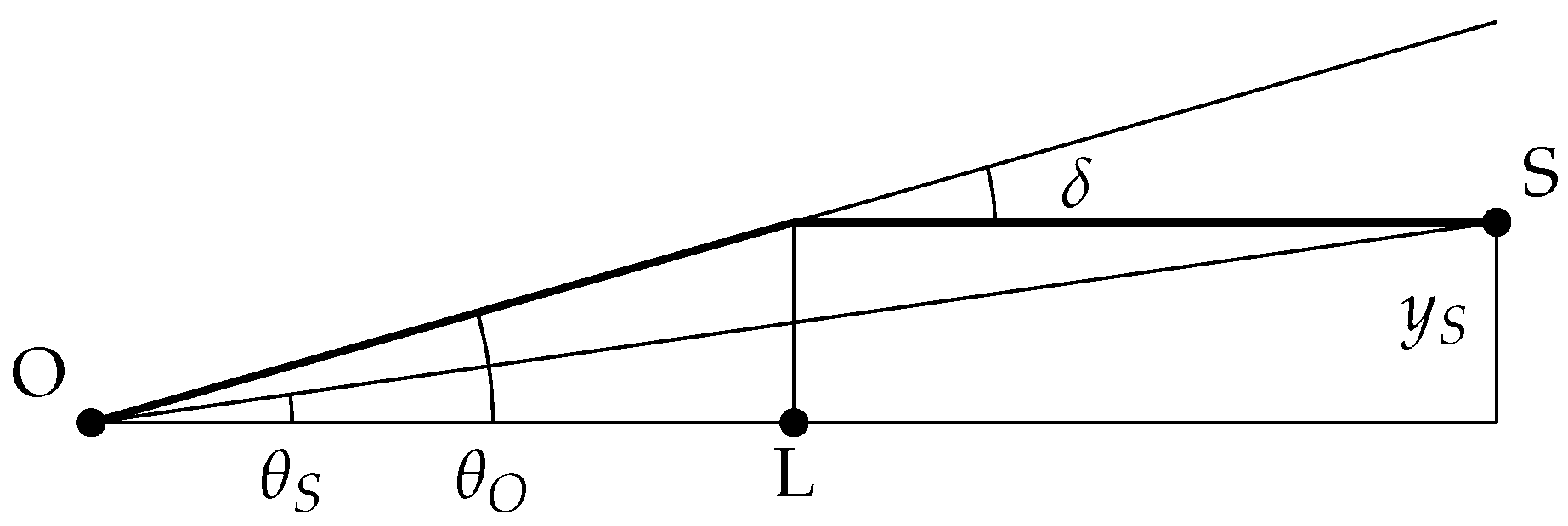
When we pass from comoving to proper distances by multiplying by the scale factor $a(x)$ we obtain:

$$y_p={\theta }_S{x}_p+\frac{a(x_p)}{a_S}(y_{pS}-{\theta }_S{x}_{pS}),$$

(42)

where we used a subscript p to indicate the proper distance. The above is not a straight line trajectory, as also noticed by the authors of Ref. [15]. It is bent because of the $a(x_p)$ factor on the right-hand side, whose effect vanishes only for $y_{pS}={\theta }_S{x}_{pS}$. The latter condition, when substituted in Equation (41), represents the ray which gets to $y=0$ when $x=0$, i.e., the observed ray. See Figure 4.

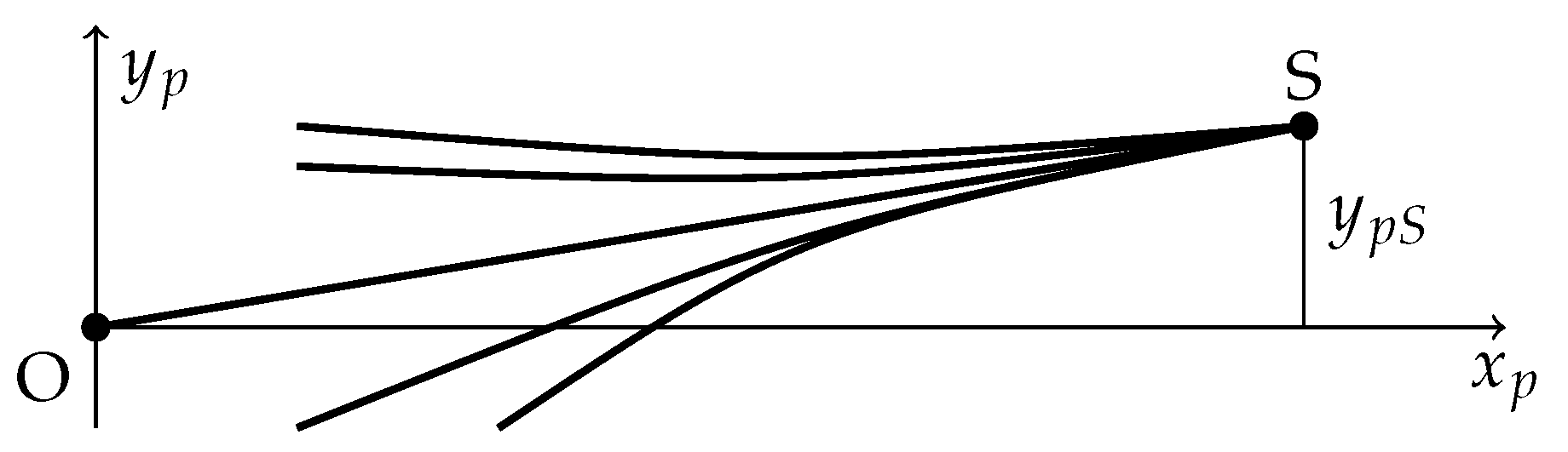
The Hubble flow seems to bend away the trajectories such that we cannot detect any light. This happens isotropically, i.e., no observer could ever detect a bent ray but just the straight one coming directly from the source.

On the other hand, let’s speculate about the following. If a cosmologically bent ray passes sufficiently close to a lens, then its trajectory could be bent back by the gravitational field of the lens, possibly allowing us to detect it. See Figure 5.

This “back-bending” seems to suggest that the bending angle must increase and therefore cosmology must somehow enter the gravitational lensing phenomenon.

3.2. Calculation of the Bending Angle

We now integrate Equation (39) retaining the first order only in α. For this reason, the $Y(X)$ entering the integral is the zeroth-order solution, which we discussed in the previous subsection.

Since we are working at the first order in α, we can assume without losing generality that the zeroth-order trajectory is horizontal, i.e., $Y^{(0)}=Y_S\equiv y_S/x_L$.

The equation for the slope, i.e., Equation (38), becomes

$$\frac{d\theta }{dX}=-\frac{\alpha Y_S}{a(X){[{(X-1)}^2+Y_S^2]}^{3/2}}.$$

(43)

In order to determine $a(X)$, we take advantage of metric (20) and write:

$$d{x}^2=\frac{1-8\mu }{1+{(dy/dx)}^2}\frac{d{t}^2}{a^2},$$

(44)

which is a very complicated integration to perform, since it includes the very trajectory we want to determine. On the other hand, we are staying at the lowest possible order of approximation; therefore:

$$dx=-\frac{dt}{a},$$

(45)

i.e., all the contributions coming from μ and θ of Equation (44) are of negligible order in Equation (43).

Now, write Equation (43) as follows:

$$d\theta =-\frac{\alpha dX}{a(X)Y_S^2{\left[1+\frac{{(X-1)}^2}{Y_S^2}\right]}^{3/2}}.$$

(46)

When ${(X-1)}^2\gg Y_S^2$, the above integration, whatever function a might be of X, is $\mathcal{O}(Y_S)$. On the other hand, when ${(X-1)}^2\ll Y_S^2$, the above integration is $\mathcal{O}(1/Y_S^2)$.

Therefore, the main contribution comes from $X=1$ and spans the interval $1-Y_S<X<1+Y_S$. That is, most of the deflection takes place very close to the lens, as it happens for the case of the Schwarzschild metric. For this reason, we also approximate $a(X)$ with $a_L$, which is the scale factor when $x=x_L$.

Therefore, we end up with the following bending angle:

$$\delta =-\frac{\alpha }{a_L{Y}_S^2}(-2Y_S)=\frac{2\alpha }{a_L{Y}_S}=\frac{4M}{a_L{y}_S}.$$

(47)

The above formula is general, valid for any kind of Hubble flow. We derive it using another method in Appendix A and prove its validity in the case of a dust-dominated universe, for which an exact calculation is possible, in Appendix B.

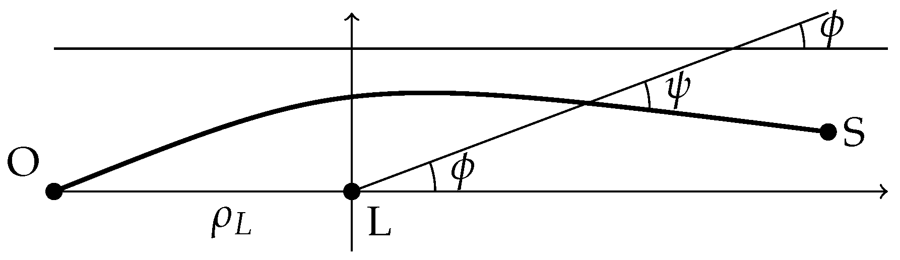
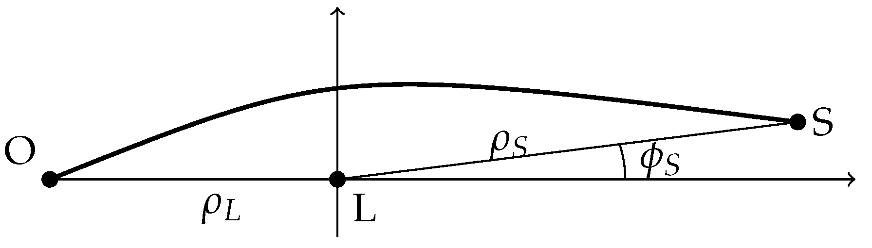
Now we apply Equation (47) in the lens equation. Let us refer to Figure 2. The geometry of this figure is justified by the fact that, as we showed earlier, the bending happens predominantly at the closest approach distance to the lens.

In Figure 2, ${\theta }_S$ is the angular position of the source, so that ${\theta }_S{D}_S$ is the proper transversal position of the source, where $D_S$ is the angular-diameter distance from the observer to the source. The angle ${\theta }_O$ is the angular apparent position of the source, so that ${\theta }_O{D}_S$ is the transversal apparent position of the source.

Therefore, the lens equation in the thin-lens approximation can be written as:

$${\theta }_O{D}_S={\theta }_S{D}_S+\delta D_{LS},$$

(48)

where $D_{LS}$ is the angular-diameter distance between lens and source. Using the result of Equation (47), we get

$${\theta }_O-{\theta }_S=\frac{4M}{a_L{y}_S}\frac{D_{LS}}{D_S}.$$

(49)

In the standard lens equation, one has the closest approach distance to the lens, let’s call it R, in place of $a_L{y}_S$. One then writes $R={\theta }_O{D}_L$ and thus finds the usual formula, see e.g., [17].

Now, since we found that the deflection occurs almost completely at the closest position to the lens, we can approximate $y_S\approx y_L$. Moreover, one also has $y_L={\theta }_O{x}_L$ and $D_L=a_L{x}_L$, from the definition of the angular-diameter distance to the lens. Thus, $a_L{y}_S\approx a_L{\theta }_O{x}_L={\theta }_O{D}_L$, and we recover the usual well-known formula:

$${\theta }_O({\theta }_O-{\theta }_S)=\frac{4M}{D_L}\frac{D_{LS}}{D_S}.$$

(50)

Therefore, we can conclude that cosmology does not modify the bending angle at the leading order of the expansion in powers of μ and θ. The cosmological “drift” discussed earlier for the zeroth-order solution is already taken into account when using angular-diameter distances so that the final result does not change.

However, sub-dominant terms do carry a cosmological signature, as we show in the next section. Here, we address the simple case of a cosmological constant-dominated universe, where analytical calculations are possible.

4. Next-to-Leading Order Contributions to the Bending Angle in the Case of a Cosmological Constant-Dominated Universe

As we saw in Equation (47), the leading contribution in the expansion for the bending angle calculated in the McVittie metric is the same as the one calculated for the Schwarzschild metric. Therefore, it is interesting to check if next-to-leading orders do carry a signature of the cosmological embedding of the point lens. We tackle this issue here in the case of a cosmological constant-dominated universe, for which exact calculations are possible, and leave a more general treatment as a future work.

When $H=H_0=$ constant, one can find an analytic expression for $a(x)$:

$$x={\int }_a^1\frac{d{a}^{\prime }}{H_0{a}^2}=\frac{1}{H_0}\left(\frac{1}{a}-1\right)=\frac{z}{H_0},$$

(51)

where in the last equality we introduced the redshift. The scale factor as function of the comoving distance is thus:

$$\frac{1}{a(x)}=H_{0}x+1=H_{0}X{x}_L+1=z_{L}X+1,$$

(52)

and Equation (43) becomes:

$$\frac{d\theta }{dX}=-\frac{\alpha Y_S(z_{L}X+1)}{{[{(X-1)}^2+Y_S^2]}^{3/2}}.$$

(53)

As we anticipated, this equation can be solved exactly and the bending angle, as we defined it in Equation (39), is the following:

$$\begin{array}{c}\hfill \delta =\frac{\alpha }{Y_S}\left[\frac{1+z_L+z_L{Y}_S^2}{\sqrt{1+Y_S^2}}+\frac{(X_S-1)(1+z_L)-z_L{Y}_S^2}{\sqrt{{(X_S-1)}^2+Y_S^2}}\right].\end{array}$$

(54)

Expanding this solution for a small impact parameter $Y_S$, one gets:

$$\begin{array}{c}\hfill \delta =\frac{2\alpha (1+z_L)}{Y_S}\left[1+Y_S^2\frac{2(z_L-1)+X_S[2+X_S(z_L-1)-4z_L]}{4(z_L+1){(X_S-1)}^2}\right],\end{array}$$

(55)

where we have already truncated $\mathcal{O}(Y_S^4)$ terms and put in evidence the leading order contribution $2\alpha (1+z_L)/Y_S$ (see Equation (47)).

Recovering the physical quantities $Y_S=y_S/x_L$, $X_S=x_S/x_L$, $\alpha =2M/x_L$ and using Equation (51) in order to express x as the redshift, we get:

$$\begin{array}{c}\hfill \delta =\frac{4M(1+z_L)}{y_S}\left[1+\frac{y_S^2}{x_L^2}\frac{2z_L^2(z_L-1)+z_S[2z_L+z_S(z_L-1)-4z_L^2]}{4(z_L+1){(z_S-z_L)}^2}\right].\end{array}$$

(56)

We already showed in the discussion leading to Equation (50) that $y_S\approx {\theta }_O{x}_L$, so that:

$$\begin{array}{c}\hfill \delta =\frac{4M}{{\theta }_O{D}_L}\left[1+{\theta }_O^2\frac{2z_L^2(z_L-1)+z_S[2z_L+z_S(z_L-1)-4z_L^2]}{4(z_L+1){(z_S-z_L)}^2}\right],\end{array}$$

(57)

and in the lens equation:

$$\begin{array}{c}\hfill {\theta }_O({\theta }_O-{\theta }_S)=\frac{4M{D}_{LS}}{D_L{D}_S}\left[1+{\theta }_O^2\frac{2z_L^2(z_L-1)+z_S[2z_L+z_S(z_L-1)-4z_L^2]}{4(z_L+1){(z_S-z_L)}^2}\right].\end{array}$$

(58)

Let’s focus on Einstein ring systems, i.e., ${\theta }_S=0$. We have in this case the mass estimate (it is actually an estimate on the product $H_{0}M$, due to the presence of the angular-diameter distances, see Ref. [17])):

$$\begin{array}{c}\hfill \frac{4M{D}_{LS}}{D_L{D}_S}={\theta }_O^2\left[1-{\theta }_O^2\frac{2z_L^2(z_L-1)+z_S[2z_L+z_S(z_L-1)-4z_L^2]}{4(z_L+1){(z_S-z_L)}^2}\right].\end{array}$$

(59)

The next-to-leading order correction is $\mathcal{O}({\theta }_O^4)$ and depends on the redshifts of the lens and of the source.

Consider, for example, the Einstein ring Q0047-2808 of the CASTLES survey, for which ${\theta }_O={2.7}^{″}$, $z_S=3.60$ and $z_L=0.48$. Substituting these numbers in Equation (59), the correction on the mass estimate is therefore

$$\frac{4M{D}_{LS}}{{\theta }_O^2{D}_L{D}_S}=1+0.12{\theta }_O^2=1+2.03·{10}^{-11}.$$

(60)

This is an extremely small correction which nonetheless depends on cosmology. Note that it is only one order of magnitude larger than the terms $\mathcal{O}({\mu }^2)$ that we have neglected in our calculations.

5. Conclusions

We investigated whether cosmology affects the gravitational lensing caused by a point mass. To this purpose, we used McVittie metric as the description of the point-like lens embedded in an expanding universe. The reason for this choice is to use a metric which properly takes into account the Hubble flow to which source, lens and observer are subject. We considered the general case in which the Hubble factor is a generic function of time and find that no contribution coming from cosmology enters the bending angle at the leading order (see Equation (47)), thus strengthening the results obtained by [13,14,15,16].

We addressed the sub-dominant contributions to the bending angle in the special case of a constant Hubble factor $H=H_0$, for which exact calculations are possible. We found that in this case cosmology does affect the bending of light, through a combination of the lens and source redshifts, given in Equation (58). This correction is of order 10⁻¹¹ for the Einstein ring Q0047-2808.

We conclude that the standard approach to gravitational lensing on cosmological distances, which consists of patching together the results coming from the Schwarzschild metric (which models the lens) and Friedmann–Lemaître-Robertson–Walker (FLRW) metric (which serves to calculate the cosmological angular diameter distances), does not require modifications.

Future developments of this investigation should address the entity subdominant orders of the expansion for the bending angle in a model-independent way. We expect the latter to depend on $H_L$, i.e., the Hubble parameter evaluated at the lens redshift. If these corrections were measurable, they might provide a new cosmological probe for determining the value of the Hubble parameter at different redshifts.

Finally, we must stress that McVittie metric is a particular and oversimplified description of the geometry of a lens, this being a galaxy or a cluster of galaxies. Therefore, another improvement would be that of tackling the analysis of the gravitational lensing and of the bending angle by constructing for the lens a density profile more realistic than a Dirac delta (i.e., the one used here for a point mass). We expect that different lens density profiles would lead to different results in the mass estimates also from the point of view of the cosmological corrections, as shown in Ref. [10] for the case of the Kottler metric.

multiple