
Strategies to Ascertain the Sign of the Spatial Curvature


1
Escola de Ciências e Tecnologia, Universidade Federal do Rio Grande do Norte, Natal 59072-970, Rio Grande do Norte, Brazil
2
Departamento de Física, Universidad Autónoma de Barcelona, Bellaterra, Barcelona 08193, Spain
*
Author to whom correspondence should be addressed.
Universe 2016, 2(4), 27; https://doi.org/10.3390/universe2040027
Submission received: 14 October 2016
/
Revised: 14 November 2016
/
Accepted: 15 November 2016
/
Published: 24 November 2016
(This article belongs to the Special Issue 100 Years of Chronogeometrodynamics: the Status of the Einstein's Theory of Gravitation in Its Centennial Year)
Abstract
:The second law of thermodynamics, in the presence of gravity, is known to hold at small scales, as in the case of black holes and self-gravitating radiation spheres. Using the Friedmann–Lemaître–Robertson–Walker metric and the history of the Hubble factor, we argue that this law also holds at cosmological scales. Based on this, we study the connection between the deceleration parameter and the spatial curvature of the metric, , and set limits on the latter, valid for any homogeneous and isotropic cosmological model. Likewise, we devise strategies to determine the sign of the spatial curvature index k. Finally, assuming the lambda cold dark matter model is correct, we find that the acceleration of the cosmic expansion is increasing today.
1. Introduction
The validity of the second law of thermodynamics for systems dominated by gravity should not be taken for granted. Gravity is a long-ranged interaction while the formulation of the second is based on the observation of ordinary systems, i.e., those dominated by short-ranged interactions. In actual fact, its validity for the former systems was studied only recently, notably in the case of black holes and self-gravitating radiation spheres. In the former case, Bekenstein demonstrated that the black-hole entropy, in addition to the entropy of the black-hole exterior, never decreases [1,2]. In the latter, it was shown that the static stable configurations of a sphere of self-gravitating radiation are those that maximize the radiation entropy [3,4]. Both instances correspond to small scale systems. Although different authors assumed it to be in order to constrain the evolution of cosmological models (see, e.g., [5] and references therein), as far as we know, the validity of the said law at large (i.e., cosmic) scales has not been explored as yet. The main purpose of this work is to fill this gap. Our study analysis rests on the simplest realistic large-scale space-time metric, namely, the Friedmann–Lemaître–Robertson–Walker (FLRW) one alongside a selected set of observational data about the history of cosmic expansion.
Homogeneous and isotropic universe models are usually described by the FLRW metric
coupled to the sources of the gravitational field. This metric relies on the cosmological principle [6,7,8] whose validity, at large scales, has not been contradicted thus far [9] and it looks rather robust [10,11,12]. The curvature index, k, is either , or depending on whether the spatial part of the metric is flat, positively curved (closed), or negatively curved (hyperbolic), respectively.
This constant index, like the scale factor , is not a directly observable quantity. In principle, however, it can be determined through the knowledge of the dimensionless, fractional curvature density, , which is accessible to observation, albeit indirectly. As usual, denotes the Hubble factor. Current measurements of only indicate that its present absolute value is small ( ≲ 10 [13,14]). Note that this constraint was obtained under the assumption that the universe is accurately described by the ΛCDM model. Thus the sign of k remains unknown.
The aim of this research is fourfold: (i) To determine whether the second law of thermodynamics is fulfilled at cosmological scales and; if so, (ii) constrain as much as possible and (iii) determine the sign of k; finally, (iv) to derive a thermodynamic constraint relating the present value of the deceleration and jerk parameters. For the first three objectives, neither a cosmological model nor theory of gravity will be assumed. We shall just use the FLRW metric, the history of the Hubble factor and the second law of thermodynamics. For the fourth objective, we will assume Einstein gravity and the ΛCDM model. As is customary, a subindex zero attached to any quantity means that the latter should be evaluated at present time.
2. Cosmological Consequences of the Second Law
Given the strong connection between gravity and thermodynamics [1,2,15,16,17], it is natural to expect that the universe behaves as a normal thermodynamic system; it therefore must tend to a state of maximum entropy in the long run [18,19].
For comoving observers, FLRW models entail “normal”, “trapped” and “anti-trapped” regions. In the first one, the expansion of outgoing null geodesic congruences, normal to the spatial two-sphere of radius centered at the origin (i.e., at the position of the observer), is positive, and negative for ingoing null geodesic congruences. In the trapped region, both kind of geodesic congruences have negative expansion. By contrast, in the anti-trapped region the expansion of both congruences is positive. The boundary hyper-surface of the space-time anti-trapped region is called the apparent horizon; its radius is . Since the observer has no information about what might be going on beyond the horizon, the latter has an entropy, namely: , where is Planck’s length. For details, see [20]. (Bear in mind that and H have dimensions of length and length, respectively, k of length, and a is dimensionless.)
A rather reasonable assumption concerning the entropy of the observable universe is that it is dominated by the entropy of the cosmic horizon. In the current universe, the entropy of the horizon exceeds that of supermassive black holes, stellar black holes, relic neutrinos and CMB photons by 18, 25, 33 and 33 orders of magnitude, respectively [21]. There are several possible choices for the cosmic horizon: the particle horizon, the event horizon, the apparent horizon and the Hubble horizon. Given that the first one does not exist for accelerating universes and the second only exists if the universe accelerates forever in the future, we take the apparent horizon, which, on the one hand, always exists, both for ever-expanding and ever-contracting universes, and, on the other hand, by contrast to the other mentioned possibilities, the laws of thermodynamics are fulfilled on it [22]. The Hubble horizon is a particular case of the apparent horizon when .
To support the above claim that the entropy of the horizon dominates over the entropy of any form of energy inside the horizon, especially at late times, we shall consider the entropy of pressureless matter. The latter is given by [23], with , being the present number density of matter particles, and
the volume enclosed by the apparent horizon for and (for the flat case, ). For one follows . Hence, when the ratio results proportional to . For one has , hence
Accordingly, in all three cases () the entropy of the horizon overwhelms that of the matter inside it, especially at late times.
Recalling that with the area of the horizon (henceforward we set ), the second law of thermodynamics leads to
where the prime means .
The second inequality tells us that if is or has been positive at any stage of cosmic expansion (excluding, possibly, the pre-Planckian era), then and that, in principle, any sign of k is compatible with . Multiplying the said inequality by produces , which can be recast in terms of the redshift as
Thus, if for all , then both and are consistent with the second law of thermodynamics at large scales. However, given the present ample uncertainties in the observational data regarding the Hubble history, if k were , then the said law could break down at cosmic scales. To explore this, we set in Equation (4) and integrate the resulting expression in the interval to get
Therefore, if this relationship failed for whatever pair of points (, ), with , it should mean that the choice would not be consistent with the second law at the said scales.
We use Equation (5) alongside the 28 experimental data H vs. z, in the interval , with their error bars, compiled by Farook et al. [24] and listed in Table 1 (see also Figure 1) for the reader convenience, to draw Figure 2. The latter suggests that, given the experimental uncertainties, the possibility also appears compatible with the inequality . While wider compilations of are available, we believe this one is preferable because it does not include any obviously correlated data, nor does it contain older, less reliable data, some with much weight from anomalously small error bars.
Equation (4) can alternatively be written as
where is the dimensionless deceleration parameter. The last equation, like (4), imposes an upper bound (that depends on redshift) on . In the radiation dominated era was close to 1; a result that, in spite of having been derived for spatially flat universes described by general relativity, should hold irrespective of the sign of the curvature and the gravity theory employed. Notice that even a mild deviation of at that time would conflict with the observational results about the primordial nucleosynthesis of light elements [25]. This suggests an easily verifiable test on modified gravity theories, namely, that they should be consistent with the bound at the radiation era. However, if general relativity is the right theory of gravity, the first Friedmann equation implies the stronger bound at all epochs. Nevertheless, even if one uses general relativity, Equation (6) might provide a useful bound when .
We can draw further consequences from the thermodynamic bound (6). To this end, we first apply the model independent Gaussian process (GP) introduced by Seikel et al. [34] to smooth the 28 observational data depicted in Figure 1. Figure 3 shows the outcome.
Inspection of the latter suggests that in the redshift range be considered. If this gets confirmed by future data of much higher quality, any sign of the curvature scalar index k will be consistent with the second law of thermodynamics. The following analysis, based on the smoothed data shown in Figure 3, allows the quantification of the gap between and .
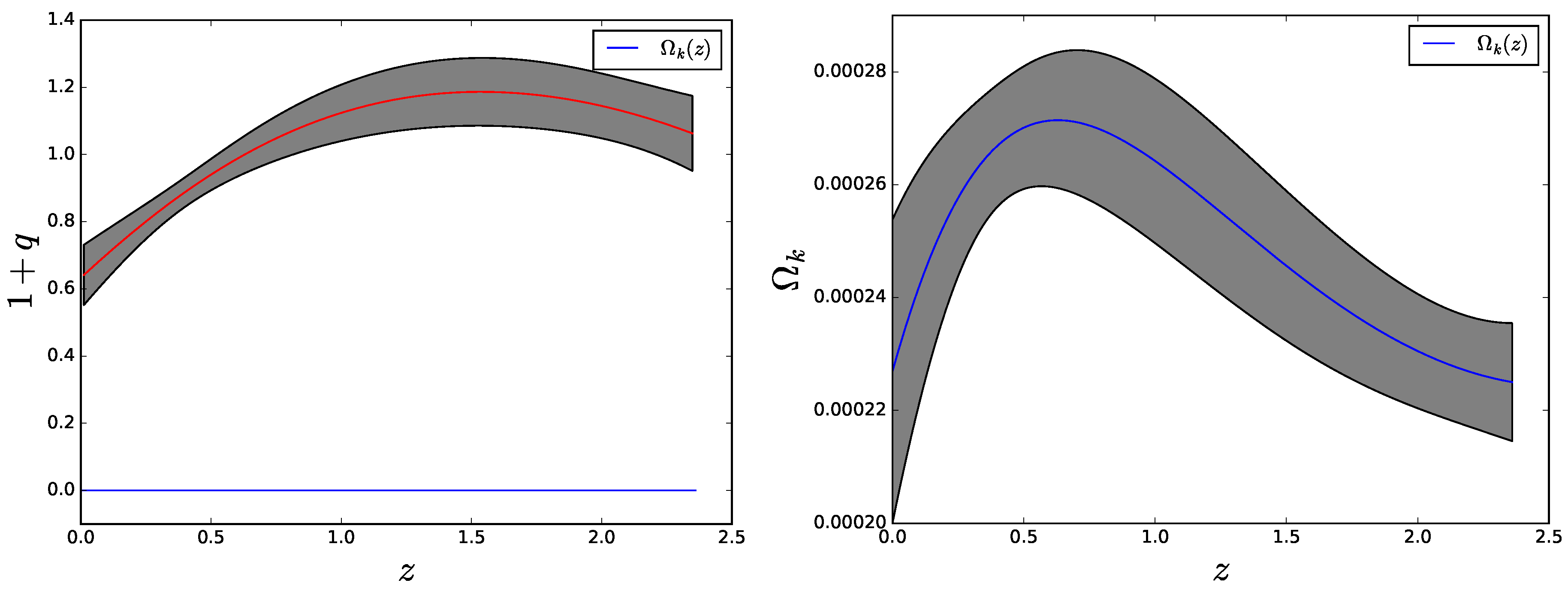
The quantity alongside its , uncertainty is obtained by computing the quantity in the left-hand side of (4) using the smoothed data, and similarly by computing using the same data. Figure 4 and Figure 5 summarize the results for and , respectively. It is apparent that, whatever the sign of k, the second law is fulfilled by a generous margin. Likewise, inspection of the left panels of the aforesaid figures indicates that . Obviously, this upper bound is much more loose than the one obtained in [14] (), but the latter is based on a particular (though so far successful) cosmological model—the ΛCDM—that rests on a number of assumptions, some of which can be justified only a posteriori. By contrast, this other rests just on the FLRW metric and the second law of thermodynamics. Combining the readings on the vertical axes of the right panels of the same figures yields the constraint .
Regrettably, as hinted above, the quality of the available sets of data is not good enough to directly constrain into a small range, much less to discriminate the sign of k. One has to apply some smoothing procedure to the data of the Hubble history (the GP process in our case) to downsize the error bars and thus obtain a tighter constraint. However, one should not be fully confident about the outcome since the said procedure, though efficient, is not exempt of potential shortcomings.
Nevertheless, the situation is expected to improve greatly in the not so distant future thanks to the Sandage–Loeb (SL) test [35,36] based on the Mc-Vittie formula [37]
that governs the drift of the redshift. Here, stands for the redshift of the source (e.g., quasar, globular cluster, HI region, ...). With the use of high precision spectrographs, such as CODEX [38], and extremely large telescopes, as the ELT [39], the SL test will provide us accurate data sets at different redshift intervals. These data will be free of any assumption whatsoever about the spatial curvature, gravity theory or cosmological model.
Observational data in the interval will be provided by the square kilometer array (SKA) radio-telescope [40], likewise the wide radio-sky survey PARKES will scan 21-cm radio-sources [41] as well as the experiment CHIME in the interval [42]. To collect a useful sample of data will take between one and four decades, approximately. Details can be found in References [43,44].
If the data revealed that, in some redshift, interval H decreased with increasing z, it would immediately imply . On the contrary, if H always increased in every z interval, the application of (4) would require more effort, but in any case it will (hopefully) permit one to discern the sign of k.
If the above strategy would fail, for instance if the data would indicate different signs for in separate intervals, it would mean either that the second law of thermodynamics does fail at large scales or that the FLRW metric should not be trusted after all.
3. The Jerk Parameter
By expanding the scale factor in terms of its successive derivatives we can write
where and are the dimensionless jerk and snap parameters, respectively.
Here, we shall focus on the current value of the jerk parameter of a universe dominated by pressureless matter and the cosmological constant (subindexes m and Λ, respectively). Thus far, we did not specialize to any cosmological model nor theory of gravity. In what follows, to constrain the theoretical value of , we adopt general relativity and the ΛCDM model because they are the simplest theory and model, respectively, that comply, at least at the background level, with the observational data [14]. In this model, the Hubble factor, as well as the deceleration and jerk parameters, read in terms of the redshift
where the various , with , and k, stand for the current values of the fractional energy densities.
Bearing in mind the Friedmann constraint we readily get
from Equation (11). Thereby if future accurate measurements show that deviates from unity, we will know that our universe (modulo the FLRW metric and the ΛCDM are correct) is not spatially flat, and the deviation will coincide with minus the present value of the spatial curvature. Unfortunately, current measurements of come along only with great latitude, [45]. However, this wide observational uncertainty gets substantially reduced after combining (12) with Equation (6), specialized to the ΛCDM model. It readily yields . For instance, using the experimental constraint on of Daly et al. [46], , we find (within )
4. Concluding Remarks
The validity of the second law, in the presence of gravity, is well supported at small scales by the thermodynamics of astrophysical-sized collapsed objects, in particular of black holes [1,2], and of self-gravitating radiation spheres [3,4] but, to the best of our knowledge, this law had not been tested at cosmological scales thus far. Here, assuming the correctness of the FLRW metric at large scales and using the history of the Hubble factor—see Equations (4) and (5) and Figure 2—we found that the second law likely holds at these scales as well. However, due to the sizable error bars of the data, the thermodynamic constraint on is rather loose. As we have shown, the situation greatly improves by applying the GP procedure of Reference [34] to these data. Then, —see the right-hand panel of Figure 4 and Figure 5. However, although the procedure rests on very reasonable assumptions, these are hard to test. On the other hand, we could not determine the sign of k. Nevertheless, we suggested that by means of Mc Vittie formula, Equation (7) of the drift of the redshift [37] and the use of advanced telescopes and spectrographs that will be in service soon, it will be possible to obtain accurate data capable of discerning it. Further, in the context of the ΛCDM model, we demonstrated a very simple relationship, Equation (12), between the present value of the jerk parameter and . Finally, we showed that the second law drastically reduces the ample uncertainty about the current value of the jerk and using current constraints on sets a lower bound on it.
Author Contributions
The authors contributed equally to this paper.
Conflicts of Interest
The authors declare no conflict of interest.
References
- Bekenstein, J.D. Generalized second law of thermodynamics in black-hole physics. Phys. Rev. D 1974, 9, 3292–3300. [Google Scholar] [CrossRef]
- Bekenstein, J.D. Statistical Black Hole Thermodynamics. Phys. Rev. D 1975, 12, 3077–3085. [Google Scholar] [CrossRef]
- Sorkin, R.D.; Wald, R.M.; Jiu, Z.Z. Entropy of Self-Gravitating Radiation. Gen. Relativ. Gravit. 1981, 13, 1127–1146. [Google Scholar] [CrossRef]
- Pavón, D.; Landsberg, P.T. Heat capacity of a self-gravitating radiation sphere. Gen. Relativ. Gravit. 1988, 20, 457–461. [Google Scholar] [CrossRef]
- Ferreira, P.C.; Pavón, D. Thermodynamics of nonsingular bouncing universes. Eur. Phys. J. C 2016, 76, 37. [Google Scholar] [CrossRef]
- Robertson, H.P. Kinematics and World-Structure. Astrophys. J. 1935, 82, 284–301. [Google Scholar] [CrossRef]
- Robertson, H.P. Kinematics and World-Structure III. Astrophys. J. 1936, 83, 257–271. [Google Scholar] [CrossRef]
- Walker, A.G. On Milne’s theory of world-structure. Proc. Lond. Math. Soc. 1936, s2-42, 90–127. [Google Scholar] [CrossRef]
- Clarkson, C.; Basset, B.; Lu, T.H.-C. A general test of the Copernican principle Phys. Rev. Lett. 2008, 101, 011301. [Google Scholar] [CrossRef] [PubMed]
- Zhang, P.; Stebbins, A. Confirmation of the Copernican principle through the anisotropic kinetic Sunyaev Zel’dovich effect. Phil. Trans. R. Soc. A 2011, 369, 5138–5145. [Google Scholar] [CrossRef] [PubMed]
- Bentivegna, E.; Bruni, M. Effects of Nonlinear Inhomogeneity on the Cosmic Expansion with Numerical Relativity. Phys. Rev. Lett. 2016, 116, 251302. [Google Scholar] [CrossRef] [PubMed]
- Saadeh, D.; Feeney, S.M.; Pontzen, A.; Peiris, H.V.; McEwen, J.D. How Isotropic is the Universe? Phys. Rev. Lett. 2016, 117, 131302. [Google Scholar] [CrossRef] [PubMed]
- Komatsu, E.; Smith, K.M.; Dunkley, J.; Bennett, C.L.; Gold, B.; Hinshaw, G.; Jarosik, N.; Larson, D.; Nolta, M.R.; Page, L.; et al. Seven-year Wilkinson Microwave Anisotropy Probe (WMAP) Observations: Cosmological Interpretation. Astrophys. J. Suppl. Ser. 2011, 192, 18. [Google Scholar] [CrossRef]
- Ade, P.R.; Aghanim, N.; Armitage-Caplan, C.; Arnaud, M.; Ashdown, M.; Atrio-Barandela, F.; Aumont, J.; Baccigalupi, C.; Banday, A.J.; Barreiro, R.B.; et al. Planck 2013 results. XVI. Cosmological parameters. Astron. Astrophys. 2014, 571, A16. [Google Scholar]
- Hawking, S.W. Black hole explosions? Nature 1974, 248, 30–31. [Google Scholar] [CrossRef]
- Jacobson, T. Thermodynamics of Spacetime: The Einstein Equation of State. Phys. Rev. Lett. 1995, 75, 1260–1263. [Google Scholar] [CrossRef] [PubMed]
- Padmanabhan, T. Gravity and the thermodynamics of horizons. Phys. Rep. 2005, 406, 49–125. [Google Scholar] [CrossRef]
- Radicella, N.; Pavón, D. A thermodynamic motivation for dark energy. Gen. Relativ. Grav. 2012, 44, 685–702. [Google Scholar] [CrossRef]
- Pavón, D.; Radicella, N. Does the entropy of the Universe tend to a maximum? Gen. Relativ. Grav. 2013, 45, 63–68. [Google Scholar] [CrossRef]
- Bak, D.; Rey, S.-J. Cosmic holography. Class. Quantum Grav. 2000, 17, L83. [Google Scholar] [CrossRef]
- Egan, C.; Lineweaver, C.L. A Larger Estimate of the Entropy of the Universe. Astrophys. J. 2010, 710, 1825–1834. [Google Scholar] [CrossRef]
- Wang, B.; Gong, Y.; Abdalla, E. Thermodynamics of an accelerated expanding universe. Phys. Rev. D 2006, 74, 083520. [Google Scholar] [CrossRef]
- Frautschi, S. Entropy in an Expanding Universe. Science 1982, 217, 593–599. [Google Scholar] [CrossRef] [PubMed]
- Farook, O.; Madiyar, F.R.; Crandall, S.; Ratra, B. Hubble Parameter Measurement Constraints on the Redshift of the Deceleration-Acceleration Transition, Dynamical Dark Energy, and Space Curvature. 2016; arXiv:1607.03537. [Google Scholar]
- Cyburt, R.H.; Fields, B.D.; Olive, K.; Yeh, T.H. Big bang nucleosynthesis: Present status. Rev. Mod. Phys. 2016, 88, 015004. [Google Scholar] [CrossRef]
- Simon, J.; Verde, L.; Jiménez, R. Constraints on the redshift dependence of the dark energy potential. Phys. Rev. D 2005, 71, 123001. [Google Scholar] [CrossRef]
- Moresco, M.; Cimatti, A.; Jimenez, R.; Pozzetti, L.; Zamorani, G.; Bolzonella, M.; Dunlop, J.; Lamareille, F.; Mignoli, M.; Pearce, H.; et al. Improved constraints on the expansion rate of the Universe up to z ∼ 1.1 from the spectroscopic evolution of cosmic chronometers. J. Cosmol. Astropart. Phys. 2012, 2012, 006. [Google Scholar] [CrossRef] [PubMed]
- Cuesta, A.J.; Vargas-Magaña, M.; Beutler, F.; Bolton, A.S.; Brownstein, J.R.; Eisenstein, D.J.; Gil-Marín, H.; Ho, S.; McBride, C.K.; Maraston, C.; et al. The clustering of galaxies in the SDSS-III Baryon Oscillation Spectroscopic Survey: Baryon acoustic oscillations in the correlation function of LOWZ and CMASS galaxies in Data Release 12. Mont. Not. R. Astron. Soc. 2016, 457, 1770–1785. [Google Scholar] [CrossRef] [Green Version]
- Blake, C.; Brough, S.; Colless, M.; Contreras, C.; Couch, W.; Croom, S.; Croton, D.; Davis, T.M.; Drinkwater, M.J.; Forster, K.; et al. The WiggleZ Dark Energy Survey: Joint measurements of the expansion and growth history at z < 1. Mon. Not. R. Astron. Soc. 2012, 425, 405–141. [Google Scholar]
- Stern, D.; Jimenez, R.; Verde, L.; Kamionkowski, M.; Adam, S. Cosmic Chronometers: Constraining the Equation of State of Dark Energy. I: H(z) Measurements. J. Cosmol. Astropart. Phys. 2010, 2010, 008. [Google Scholar] [CrossRef]
- Moresco, M. Raising the bar: New constraints on the Hubble parameter with cosmic chronometers at z∼2. Mon. Not. R. Astron. Soc. 2015, 450, L16–L20. [Google Scholar] [CrossRef]
- Delubac, T.; Bautista, J.E.; Busca, N.G.; Rich, J.; Kirkby, D.; Bailey, S.; Font-Ribera, A.; Slosar, A.; Lee, K.-G.; Pieri, M.M.; et al. aryon acoustic oscillations in the Lyα forest of BOSS DR11 quasars. Astron. Astrophys. 2015, 574, A59. [Google Scholar] [CrossRef] [Green Version]
- Font-Ribera, A.; Kirkby, D.; Busca, N.; Miralda-Escudé, J.; Ross, N.P.; Slosar, A.; Rich, J.; Aubourg, E.; Bailey, S.; Bhardwaj, V.; et al. Quasar-Lyman α forest cross-correlation from BOSS DR11: Baryon Acoustic Oscillations. J. Cosmol. Astropart. Phys. 2014, 2014, 027. [Google Scholar] [CrossRef]
- Seikel, M.; Clarkson, C.; Smith, M. Reconstruction of dark energy and expansion dynamics using Gaussian processes. J. Cosmol. Astropart. Phys. 2012, 2012, 036. [Google Scholar] [CrossRef]
- Sandage, A. The Change of Redshift and Apparent Luminosity of Galaxies due to the Deceleration of Selected Expanding Universes. Astrophys. J. 1962, 136, 319–333. [Google Scholar] [CrossRef]
- Loeb, A. The Change of Redshift and Apparent Luminosity of Galaxies due to the Deceleration of Selected Expanding Universes. Astrophys. J. 1998, 499, L111–L114. [Google Scholar] [CrossRef] [Green Version]
- Vittie, G.C.M. Cosmological Theory, 2nd ed.; Wiley: New York, NY, USA, 1949. [Google Scholar]
- Spectrograph CODEX. Available online: http://www.iac.es/proyecto/codex/ (accessed on 22 November 2016).
- The European Extremely Large Telescope. Available online: http://www.eso.org/public/teles-instr/e-elt/ (accessed on 22 November 2016).
- Klockner, H.R.; Obreschkow, D.; Martins, C.; Raccanelli, A.; Champion, D.; Roy, A.; Lobanov, A.; Wagner, J.; Keller, R. Real time cosmology-A direct measure of the expansion rate of the Universe with the SKA. Proc. Sci. 2015, AASKA14, 027. [Google Scholar]
- Parkers 21 cm Multibeam Project. Available online: http://www.atnf.csiro.au/research/multibeam/ (accessed on 22 November 2016).
- The Canadian Hydrogen Intensity Mapping Experiment. Available online: chime.phas.ubc.ca/ (accessed on 22 November 2016).
- Yu, H.R.; Zhang, T.J.; Pen, U.L. Method for Direct Measurement of Cosmic Acceleration by 21-cm Absorption Systems. Phys. Rev. Lett. 2014, 113, 041303. [Google Scholar] [CrossRef] [PubMed]
- Liske, J.; Grazian, A.; Vanzella, E.; Dessauges, M.; Viel, M.; Pasquini, L.; Haehnelt, M.; Cristiani, S.; Pepe, F.; Avila, G.; et al. Cosmic dynamics in the era of Extremely Large Telescopes. Mon. Not. R. Astron. Soc. 2008, 386, 1192–1218. [Google Scholar] [CrossRef]
- Bochner, B.; Pappas, D.; Dong, M. Testing Lambda and the Limits of. Cosmography with the Union2.1. Supernova Compilation. Astrophys. J. 2015, 814, 7. [Google Scholar] [CrossRef]
- Daly, R.; Djorgovski, S.G.; Freeman, K.A.; Mory, M.P.; O’Dea, C.P.; Kharb, P.; Baum, S. Improved Constraints on the Acceleration History of the Universe and the Properties of the Dark Energ. Astrophys. J. 2008, 677, 1–11. [Google Scholar] [CrossRef]
- Perlmutter, S.; Aldering, G.; Della Valle, M.; Deustua, S.; Ellis, R.S.; Fabbro, S.; Fruchter, A.; Goldhaber, G.; Groom, D.E.; Hook, I.M.; et al. Discovery of a supernova explosion at half the age of the Universe. Nature 1998, 391, 51–54. [Google Scholar] [CrossRef] [Green Version]
- Riess, A.G.; Kirshner, R.P.; Schmidt, B.P.; Jha, S.; Challis, P.; Garnavich, P.M.; Esin, A.A.; Carpenter, C.; Grashius, R.; Schild, R.E.; et al. BV RI light curves for 22 type Ia supernovae. Astron. J. 1999, 117, 707–724. [Google Scholar] [CrossRef]
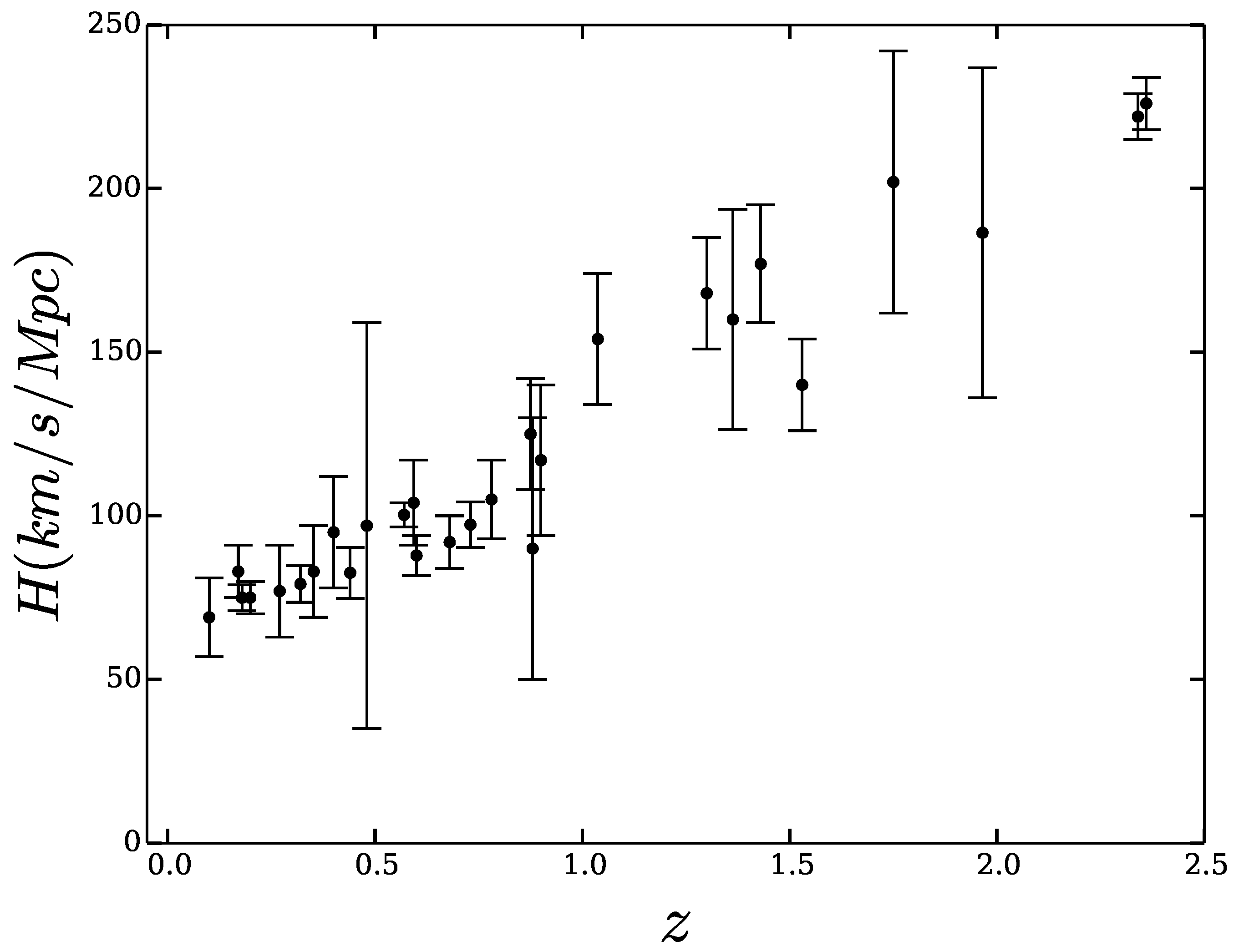
Figure 1.
28 data points with their uncertainty.

Figure 2.
Left-hand side vs. right-hand side of Equation (5) for all possible combinations of the data shown in Table 1. The error bars denote confidence level.
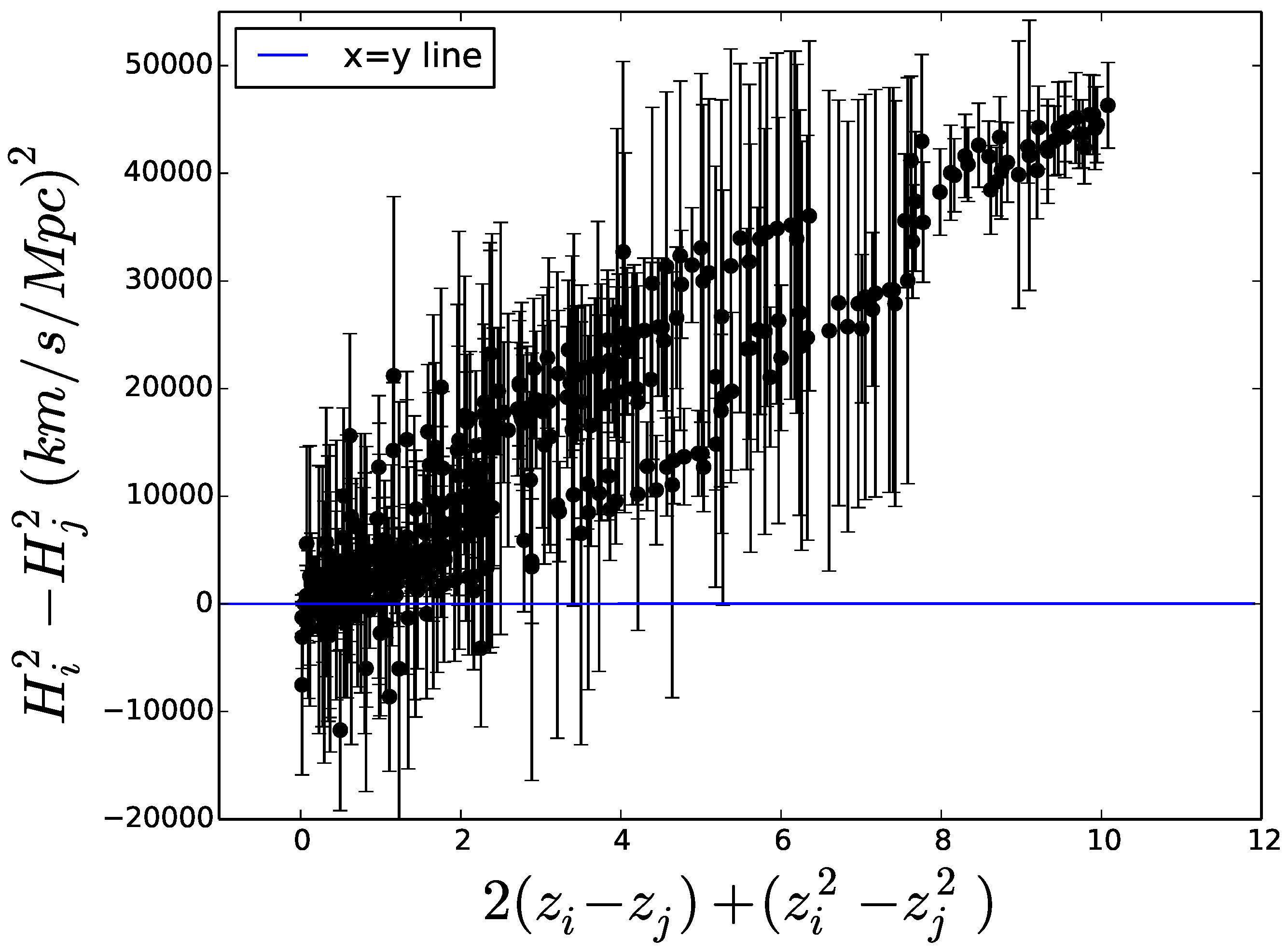
Figure 3.
Gaussian process reconstruction of the history of the Hubble factor from the raw data depicted in Figure 1, as well as here for convenience of the reader. The blue shaded region shows the uncertainty.
Figure 3.
Gaussian process reconstruction of the history of the Hubble factor from the raw data depicted in Figure 1, as well as here for convenience of the reader. The blue shaded region shows the uncertainty.
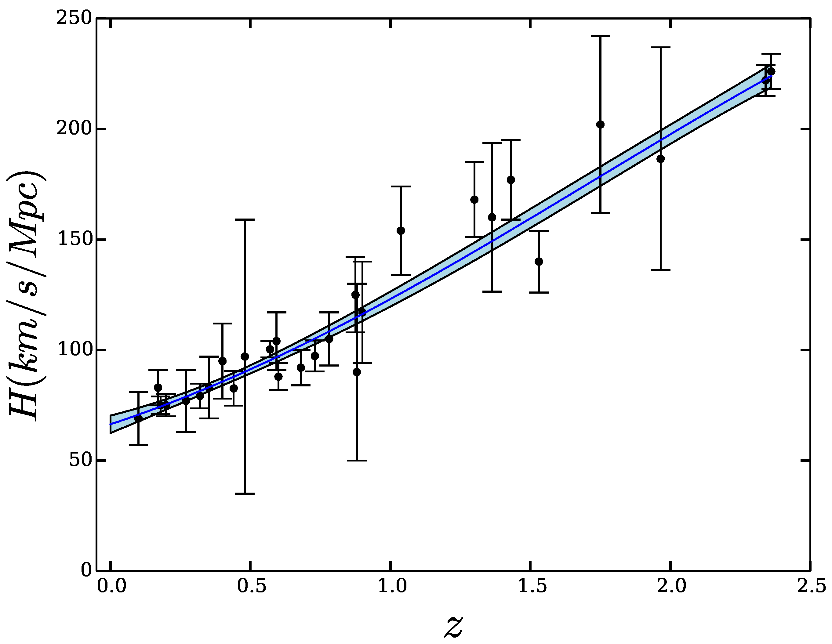
Figure 4.
Left panel: vs. redshift after smoothing the 28 data as depicted in Figure 3. Also shown is for . Clearly, the latter is practically zero. Right panel: Zoom of and its uncertainty interval.
Figure 4.
Left panel: vs. redshift after smoothing the 28 data as depicted in Figure 3. Also shown is for . Clearly, the latter is practically zero. Right panel: Zoom of and its uncertainty interval.
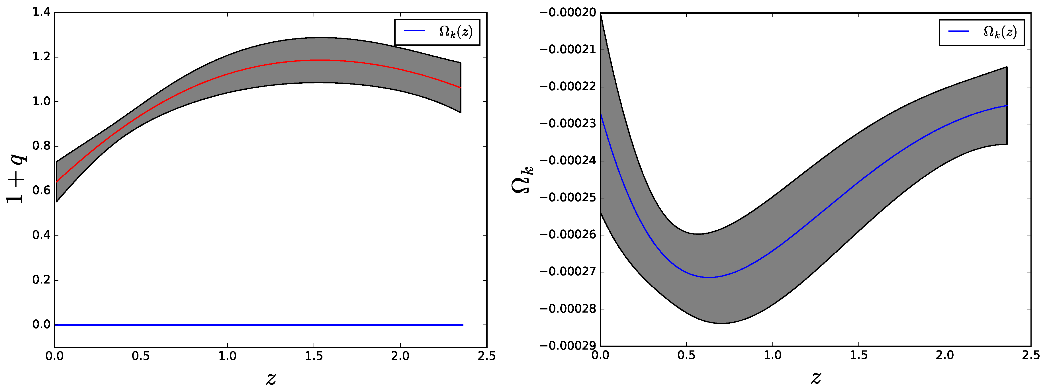
Figure 5.
Same as Figure 4 but for .
Figure 5.
Same as Figure 4 but for .


© 2016 by the authors; licensee MDPI, Basel, Switzerland. This article is an open access article distributed under the terms and conditions of the Creative Commons Attribution (CC-BY) license (http://creativecommons.org/licenses/by/4.0/).
Share and Cite
MDPI and ACS Style
Ferreira, P.C.; Pavón, D. Strategies to Ascertain the Sign of the Spatial Curvature. Universe 2016, 2, 27. https://doi.org/10.3390/universe2040027
AMA Style
Ferreira PC, Pavón D. Strategies to Ascertain the Sign of the Spatial Curvature. Universe. 2016; 2(4):27. https://doi.org/10.3390/universe2040027
Chicago/Turabian StyleFerreira, Pedro C., and Diego Pavón. 2016. "Strategies to Ascertain the Sign of the Spatial Curvature" Universe 2, no. 4: 27. https://doi.org/10.3390/universe2040027
Note that from the first issue of 2016, this journal uses article numbers instead of page numbers. See further details here.