3-Form Cosmology: Phantom Behaviour, Singularities and Interactions

Abstract

The latest cosmological observations by the Planck collaboration (and combined with others) are compatible with a phantom-like behaviour ($w<-1$) for the dark energy equation of state that drives the current acceleration of the Universe. With this mindset, we look into models where dark energy is described by a 3-form field minimally coupled to gravity. When compared to a scalar field, these models have the advantage of more naturally accommodating a cosmological-constant and phantom-like behaviours. We show how the latter happens for a fairly general class of positive-valued potentials, and through a dynamical system approach, we find that in such cases the 3-form field leads the Universe into a Little Sibling of the Big Rip singular event into the future. In this work, we explore the possibility of avoiding such singularity via an interaction in the dark sector between cold dark matter and the 3-form field. For the kind of interactions considered, we deduce a condition for replacing the LSBR by a late time de Sitter phase. For specific examples of interactions that meet this condition, we look for distinctive imprints in the statefinder hierarchy $\{{S_3}^{\left(1\right)};{S_4}^{\left(1\right)}\}$, $\{{S_3}^{\left(1\right)};{S_5}^{\left(1\right)}\}$, and in the growth rate of matter, $ϵ\left(z\right)$, through the composite null diagnostic (CND).

1. Introduction

Although it has been almost two decades since the supernova measurements [1,2] that led to the discovery of the current acceleration of the expansion of the universe, few advances have been made on the nature of the so-called dark energy (DE)—the fluid that drives this acceleration and comprises about 70% of the energy density of the Universe. In fact, the ΛCDM model—which is favoured by most observations—does little to alleviate this issue, offering no answers as to why the value of the cosmological constant Λ is so small when compared to the expected value from quantum field theory (cosmological constant problem) or why the energy densities of DE and of dark matter (DM) are on the same order of magnitude today (coincidence problem). In order to overcome these theoretical shortcomings of ΛCDM, various alternative descriptions of DE were presented along the years, from models with dynamical fields (e.g., quintessence, K-essence, etc.) to modified theories of gravity [3,4,5]. Among these proposals, we encounter the 3-form field [6,7,8,9], which has been the focus of attention in recent years, both in the context of late-time DE and in early inflation [6,7,8,9,10,11,12,13,14,15,16,17,18]. This identification of DE with a 3-form comes somewhat naturally given the well established equivalence between a massless 3-form field and a cosmological constant [19]. Therefore, by considering a 3-form field $A_{\mu \nu \rho }$ minimally coupled to gravity and with an appropriate potential V, we can obtain a richer behaviour for DE and achieve late-time acceleration in a dynamical way. In particular, we find that a 3-form can easily accommodate phantom-like behaviour ($P\le -\rho$), even for positive-valued potentials (in Ref. [20] in is shown that scalar–tensor models can also induce naturally phantom-like behaviour). We remind the reader that this kind of behaviour was found as the best fit for the Planck data when the wCDM model is considered, as the central and mean values satisfy $w<-1$ [5].

In this work, we focus precisely on such kind of potentials. As noted in [18], in many cases where the 3-form presents a phantom-like behaviour, the late-time de Sitter stage can be replaced by a Little Sibling of the Big Rip (LSBR) event in the future [21,22]. This leads to a divergence of the scale factor and the Hubble rate at an infinite cosmic time and to the dissociation of local bounded structures in our Universe at finite cosmic time, though the cosmic time derivatives of the Hubble rate remain finite. This effect was found to be scale-dependent, with the larger structures being destroyed first [21]. In order to avoid this doomsday scenario for the fate of the Universe, we consider an interaction between DM and DE (previous works on DM/3-form interaction include [10,11,12]). Models of interaction between DM and DE have long since been proposed, and an argument of natureless can be made for such interactions: if little is know about the properties of DM and DE, then why would we disregard the possibility that the two fluids that dominate the energy content of the Universe interact [23]?

Using a dynamical system approach, we look to identify the kinds of interactions that can remove the LSBR. While a dynamical systems approach has been employed in systems with 3-form since the early papers of Koivisto and Nunes [6,8,9], the existence of fixed points corresponding to infinite amplitudes of the 3-form field were overlooked in the literature. By using a set of compact variables, we were able to identify and characterise such points for the first time. In particular, we have shown how some of these points are of repulsive nature and therefore correspond to the asymptotic past of the system [18]. Once the appropriate interactions to remove the LSBR were identified, we showed how two graphic methods—the statefinder hierarchy [24] and the composite null diagnostic (CND) [25]—can be used to differentiate and observationally constrain each model. These two methods combine information about the evolution of the system at the level of the background and first order in perturbations to produce a distinctive profile, with the interesting advantage of allowing an easy qualitative analysis of how much the model deviates from ΛCDM.

2. 3-Form Cosmology and the Little Sibling of the Big Rip

In a spatially flat FLRW cosmology, only the space-like components of the 3-form are non-zero. Following [6,7,8,9], we use the parametrization $A_{ijk}=a^3\left(t\right)\chi \left(t\right){ϵ}_{ijk}$, where t is the cosmic time, $a\left(t\right)$ is the scale factor, $\chi \left(t\right)$ is a comoving scalar quantity associated with the amplitude of the 3-form field, and ${ϵ}_{ijk}=+1(-1)$ if $ijk$ is an even (odd) permutation of 123. If we consider the Universe to be filled only by a 3-form, the Friedmann and Raychaudhuri equations read, respectively [6,8,9]:

$$\begin{array}{cccc}\hfill H^2& =\frac{{\kappa }^2}{3}\left[\frac{1}{2}{\left(\dot{\chi }+3H\chi \right)}^2+V\right]=\frac{{\kappa }^2}{3}{\rho }_{\chi },\hfill & \hfill \dot{H}& =-\frac{{\kappa }^2}{2}\chi V_{,\chi }=-\frac{{\kappa }^2}{2}\left({\rho }_{\chi }+P_{\chi }\right),\hfill \end{array}$$

(1)

while the evolution of the field χ is dictated by the equation [6,7,8,9]:

$$\begin{array}{cc}\hfill \ddot{\chi }+3H\dot{\chi }+\left(1-\frac{{\chi }^2}{{\chi }_{\mathrm{c}}^2}\right)V_{,\chi }& =0.\hfill \end{array}$$

(2)

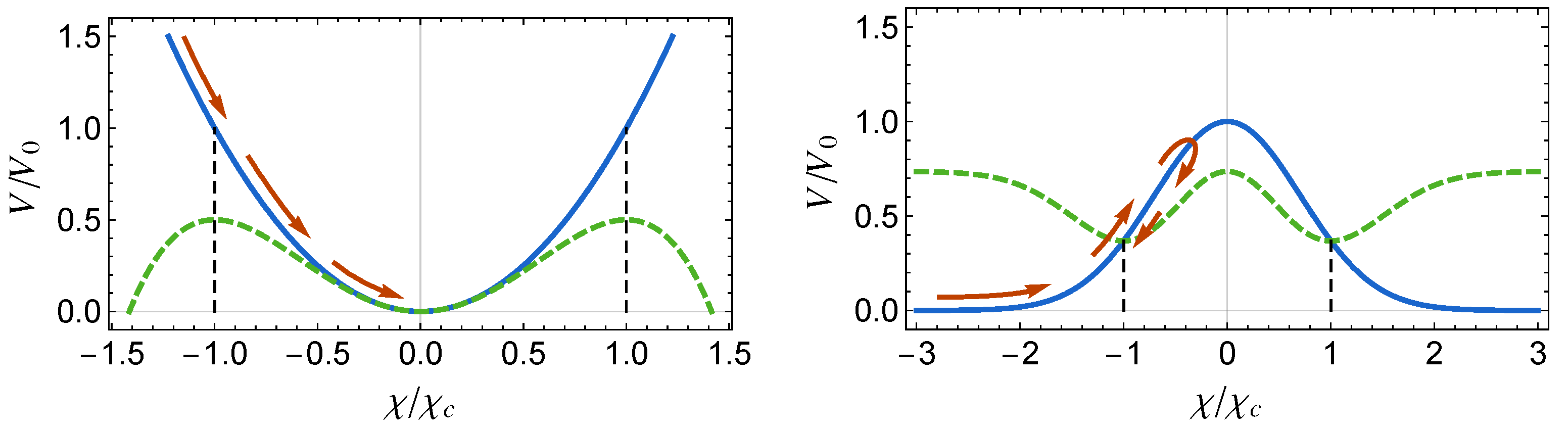
Here, a dot indicates a derivative with respect to the cosmic time, ${\kappa }^2=8\pi G$, where G is the gravitational constant, $H=\dot{a}/a$ is the Hubble rate, ${\rho }_{\chi }$ and $P_{\chi }$ are the energy density and pressure of the 3-form, ${\chi }_{\mathrm{c}}=\sqrt{2/\left(3{\kappa }^2\right)}$ and $V_{,\chi }=dV/d\chi$. Notice that the 3-form mimics a cosmological constant $(P_{\chi }=-{\rho }_{\chi })$ whenever the derivative of the potential vanishes, and presents a phantom-like behaviour $(P_{\chi }<-{\rho }_{\chi })$ when $\chi V_{,\chi }<0$ (i.e., for potentials decreasing with ${\chi }^2$).

The points $\chi =\pm {\chi }_{\mathrm{c}}$ play a critical role in 3-form cosmology, as the Friedmann Equation (1) imposes that—for expanding cosmologies ($H>0$) and positive potentials—the field χ must decay monotonically until it enters the interval $[-{\chi }_{\mathrm{c}},{\chi }_{\mathrm{c}}]$, from which it does not escape [8,9,18]. These points are static solutions of Equation (2), and represent stable (unstable) states of equilibrium of the system whenever $\partial V/\partial {\chi }^2={\left(2\chi \right)}^{-1}\partial V/\partial \chi$ is negative (positive) at $\chi =\pm {\chi }_{\mathrm{c}}$ [18]. This behaviour is illustrated in Figure 1 for two different potentials. In the case where these critical points represent stable equilibrium points, we find that as $\chi \to \pm {\chi }_{\mathrm{c}}$, the field χ saturates the Friedmann Equation (1), driving the Hubble rate to infinity, while the time derivative of the Hubble rate remains finite-valued [18]:

$$\begin{array}{c}\hfill {\dot{H}}_{(\chi \to \pm {\chi }_{\mathrm{c}})}=-\frac{2}{3}{V}_{,{\chi }^2}\left(\pm {\chi }_{\mathrm{c}}\right).\end{array}$$

(3)

Since this divergence of the Hubble rate happens in the asymptotic future, we come to the conclusion that the Universe can evolve towards a Little Sibling of the Big Rip (LSBR) event. This behaviour was first identified in [21], where it was found that while the divergence of H happens at infinite cosmic time, it leads to a dissociation of gravitationally-bound systems at a finite time. We note that the presence of a non-interacting DM component does not alter this fate. In that case, terms proportional to the energy density of DM, ${\rho }_m$, would appear on the right-hand side of Equations (1) and (2). However, as the Universe expands, ${\rho }_m$ decays like $1/a^3$; therefore, the contribution of DM becomes negligible in the far future and the system evolves as if it was not present.

3. Removing the LSBR

While the presence of non-interacting DM does not prevent the Universe from heading to a LSBR event in the future when the critical points $\pm {\chi }_{\mathrm{c}}$ represent stable equilibrium states, it is still possible that such a fate can be prevented by an appropriate interaction between the 3-form and DM. In order to study this possibility, we introduced an interaction term Q in the evolution equations [11,18]:

$$\begin{array}{cccc}\hfill {\dot{\rho }}_m+3H{\rho }_m& =-Q,\hfill & \hfill \ddot{\chi }+3H\dot{\chi }+\left(1-\frac{{\chi }^2}{{\chi }_{\mathrm{c}}^2}\right)V_{,\chi }& =\frac{\chi }{{\chi }_{\mathrm{c}}^2}{\rho }_m+\frac{Q}{\dot{\chi }+3H\chi },\hfill \end{array}$$

(4)

in such a way that the conservation of the total energy density is respected. The sign of Q in (4) indicates whether the energy transfer is from DM to the 3-form field $(Q>0)$ or from the 3-form to DM $(Q<0)$. In order to better understand the effects of such an interaction on the system, we employed a dynamical system approach based on the variables [11,18]

$$\begin{array}{cccccccc}\hfill u& \equiv {\displaystyle \frac{2}{\pi }}arctan\left({\displaystyle \frac{\chi }{{\chi }_{\mathrm{c}}}}\right),\hfill & \hfill y& \equiv {\displaystyle \frac{\dot{\chi }+3H\chi }{3H{\chi }_{\mathrm{c}}}},\hfill & \hfill z& \equiv \sqrt{{\displaystyle \frac{{\kappa }^{2}V}{3H^2}}},\hfill & \hfill s& \equiv \sqrt{{\displaystyle \frac{{\kappa }^2{\rho }_m}{3H^2}}},\hfill \end{array}$$

(5)

which are defined in the intervals $-1\le u\le 1$, $-1\le y\le 1$, $0\le z\le 1$, $0\le s\le 1$ , and respect the Friedmann constraint $y^2+z^2+s^2=1$. The set of evolution equations for the system ($u,y,z$) within the half-cylinder defined by $-1\le u\le 1$, $y^2+z^2\le 1$ and $0\le z\le 1$ is [11,18]:

$$\begin{array}{cc}\hfill u^{\prime }& =\frac{6}{\pi }{cos}^2\left(\frac{\pi u}{2}\right)\left[y-tan\left(\frac{\pi u}{2}\right)\right],\hfill \end{array}$$

(6)

$$\begin{array}{cc}\hfill y^{\prime }& =\frac{1}{2}\left\{3\left[1-y^2-z^2\right]y+\lambda \left(u\right)z^2\left[1-tan\left(\frac{\pi }{2}u\right)y\right]\right\}+\frac{{\kappa }^2}{6y{H}^3}Q,\hfill \end{array}$$

(7)

$$\begin{array}{cc}\hfill z^{\prime }& =\frac{1}{2}z\left\{3\left[1-y^2-z^2\right]-\lambda \left(u\right)\left[y-tan\left(\frac{\pi }{2}u\right)\left(1-z^2\right)\right]\right\}.\hfill \end{array}$$

(8)

Here, $\lambda \equiv -\sqrt{6/{\kappa }^2}{V}_{,\chi }/V$, and a prime indicates a derivative with regards to the logarithm of the scale factor. We considered a generic quadratic interaction and a Gaussian potential:

$$\begin{array}{cccc}\hfill Q& =3H\left({\rho }_m+{\rho }_{\chi }\right)\sum _{i=0}^2{\alpha }_i{\left(\frac{{\rho }_{\chi }}{{\rho }_m+{\rho }_{\chi }}\right)}^i,\hfill & \hfill V& =V_{0}exp\left[-{\displaystyle \frac{2\xi }{9}}{\left(\frac{\chi }{{\chi }_{\mathrm{c}}}\right)}^2\right],\hfill \end{array}$$

(9)

where ${\alpha }_i$ are dimensionless couplings that determine the strength of the interaction and $V_0$ and ξ are positive constants. The interaction term in (9) can be viewed as a generalisation of various interactions frequently considered in the literature, and has the advantage of allowing the closure of the system (6)–(8) as $Q=9H^3/{\kappa }^2{\sum }_{i=0}^2{\alpha }_i{(y^2+z^2)}^i$. At the same time, the Gaussian potential guarantees the desired behaviour for the 3-form in the non-interacting case: the 3-form behaves as an effective cosmological constant in the distant past, while in the future its phantom-like behaviour leads the Universe towards an LSBR event.

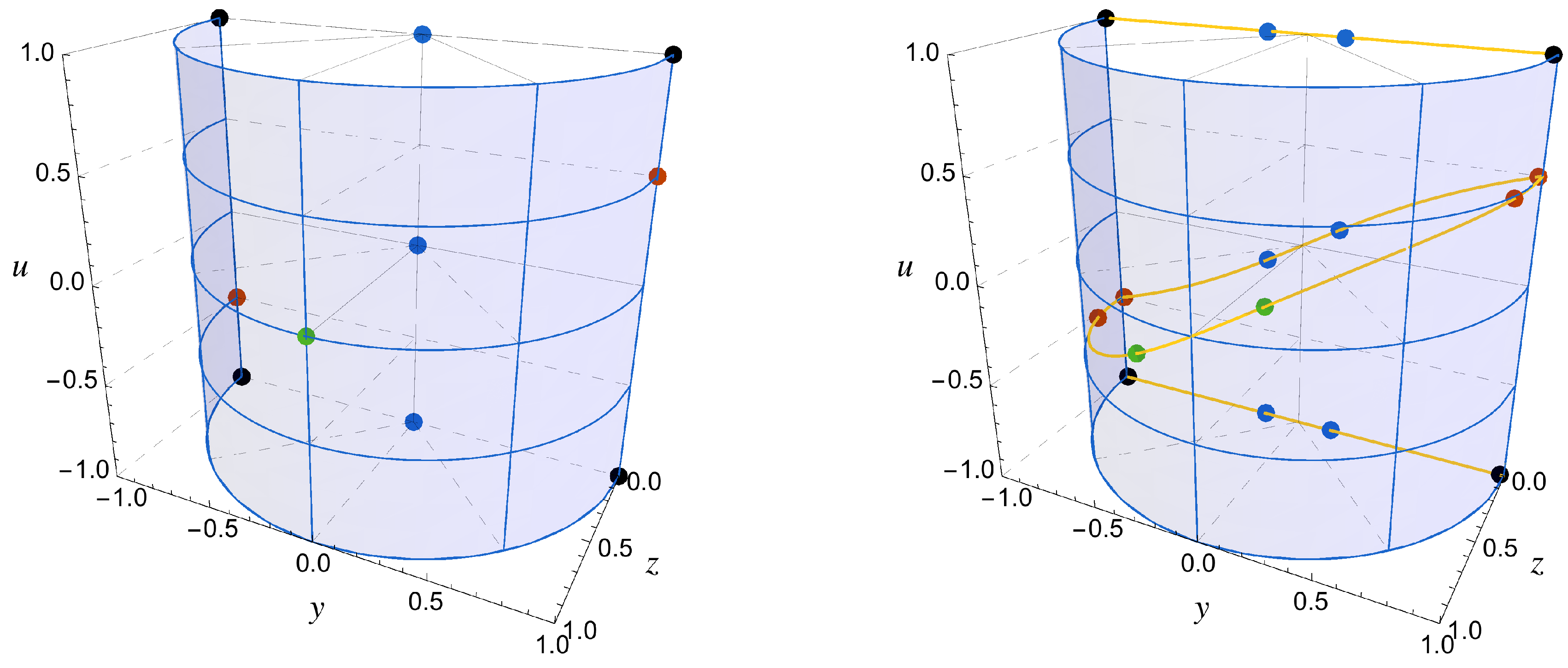
The fixed points of this system, $(u_{fp},y_{fp},z_{fp})$, can be separated into three categories:

• Fixed points verifying $z_{fp}=0$ for finite values of the 3-form field χ ($u_{fp}\ne \pm 1$). This category includes the fixed points that correspond to the future LSBR event: $(\pm 1/2,\pm 1,0)$.
• Fixed points verifying $z_{fp}\ne 0$ for finite values of the 3-form field χ ($u_{fp}\ne \pm 1$). In the non-interacting case, the fixed points of Type II correspond to extrema of the potential in the interval $]-{\chi }_{\mathrm{c}},{\chi }_{\mathrm{c}}[$.
• Fixed points that are characterized by $u=\pm 1$; i.e., infinite values of the 3-form field χ. The fixed points of Type III with a repulsive nature represent the asymptotic past of the system [18]. The position of these fixed points needs to be analysed with care and must take into account the behaviour of V—and therefore of z—as $u\to \pm 1$ [18,26].

In the left panel of Figure 2, we present the fixed points of the system in the absence of interaction: one Type I saddle point at the origin $(0,0,0)$ (blue) corresponding to a matter dominated era; two Type I points at $(\pm 1/2,\pm 1,0)$ which are attractors for the Gaussian potential and therefore correspond to the LSBR event (red); one Type II point at $(0,0,1)$ that corresponds to a potential dominated de Sitter era (green) and which is unstable for the Gaussian potential; two Type III repulsive points at $(\pm 1,0,0)$ that represent the asymptotic past matter era of the system (blue); and four Type III saddle points at $(\pm 1,+1,0)$ and $(\pm 1,1,0)$ (black). In the right panel of the same figure, we present the possible effects that the interaction can have in the position of the fixed points of the system: depending on the combination of the parameters ${\alpha }_i$, each solution can be decomposed in a pair of new fixed points which are slightly shifted from the original position.

It turns out that when there is no interaction, the position of the fixed points is given by an algebraic equation with degenerate roots. When the interaction is switched on, this degeneracy is broken and new fixed points appear. In particular, we find that if the position of the points $(\pm 1/2,\pm 1,0)$ (the red points in Figure 2, left panel) is not affected when the interaction is turned on, then their stability also does not change and the fate of the Universe remains an LSBR event. However, if and when these points are decomposed (as seen on the right panel of Figure 2), we obtain two new scaling solutions with almost complete 3-form domination (${\rho }_m/{\rho }_{\chi }\simeq |{\alpha }_0+{\alpha }_1+{\alpha }_2|\ll 1$): the first one is characterized by $z_{fp}=0$, $P_{tot}/{\rho }_{tot}\gtrsim -1$ and corresponds to a saddle point, therefore being physically uninteresting for the future evolution of the system; the second one represents an attractive de Sitter phase ($P_{tot}=-{\rho }_{tot}$) which replaces the LSBR.

We found that even with small coupling coefficients ($|{\alpha }_i|\ll 1$), an interaction of the type (9) can successfully remove the LSBR unless

$$\begin{array}{c}\hfill {\alpha }_0+{\alpha }_1+{\alpha }_2=0,\end{array}$$

(10)

which implies $Q\propto {\rho }_m^i$, for $i\ge 1$ (cf. Equation (9)). This result can be interpreted in light of the fact that the interactions that are proportional to a power of the energy density of DM do not prevent the complete decay of ${\rho }_m$ in the asymptotic future. Therefore, at late time, the system evolves as if only the 3-form were present and the Universe heads towards an LSBR event. A thorough examination of the effects of the interaction (9) on the position and stability of the fixed points of the system can be found in [18].

4. Distinguishing Interactions

The Inequality (10) defines vast subclass of interactions (9) that can successfully remove the LSBR event as the fate of the Universe in the DM/3-form model of Section 3. In order to distinguish between interactions within that subclass, we employ the statefinder hierarchy [24] and the composite null diagnostic (CND) [25]—two graphic methods constructed to obtain distinctive imprints of the cosmological evolution of a model that closely resembles ΛCDM at the present time.

The statefinder hierarchy is rooted on a cosmographic expansion of the scale factor [27,28,29]. By combining the cosmographic parameters $A_n$, where $A_n\equiv {\left(a{H}^n\right)}^{-1}({\partial }^{n}a/\partial t^n)$ for $n\ge 2$, it is possible to define the statefinder parameters [24]

$$\begin{array}{cccccc}\hfill S_3^{\left(1\right)}=& A_3,\hfill & \hfill S_4^{\left(1\right)}=& A_4+3\left(1-A_2\right),\hfill & \hfill S_5^{\left(1\right)}=& A_5-2\left(4-3A_2\right)\left(1-A_2\right),\hfill \end{array}$$

(11)

so that ${S_n}^{\left(1\right)}{|}_{\Lambda \mathrm{CDM}}=1$ for all n. The statefinder hierarchy method then consists of mapping the trajectory of the system on the planes $\{{S_3}^{\left(1\right)};{S_4}^{\left(1\right)}\}$ and $\{{S_3}^{\left(1\right)};{S_5}^{\left(1\right)}\}$, noting that the distance to the point $\{1;1\}$ provides a measure of how much the model differs from $\Lambda \mathrm{CDM}$ [24].

While the statefinder hierarchy only traces the evolution of FLRW background quantities, the CND [25] makes use of linear perturbation theory to map the evolution of the statefinder parameters against that of the growth factor $ϵ\left(x\right)$

$$\begin{array}{c}\hfill ϵ\left(x\right)\equiv \frac{f\left(x\right)}{f_{\Lambda \mathrm{CDM}}\left(x\right)}.\end{array}$$

(12)

This parameter compares the growth rate of structure $f\left(x\right)\equiv (\partial {\delta }_m/\partial x)/{\delta }_m$ of a model against that of ΛCDM, so that by construction ${ϵ\left(x\right)|}_{\Lambda \mathrm{CDM}}=1$. Here, ${\delta }_m\equiv \delta {\rho }_m/{\rho }_m$ is the matter density contrast and $\delta {\rho }_m$ is the linear perturbation of the energy density of DM [25,30]. By mapping the trajectory of the model on the plane, $\{ϵ;{S_3}^{\left(1\right)}\}$, the CND defines a new profile of the model that complements that of the statefinder hierarchy.

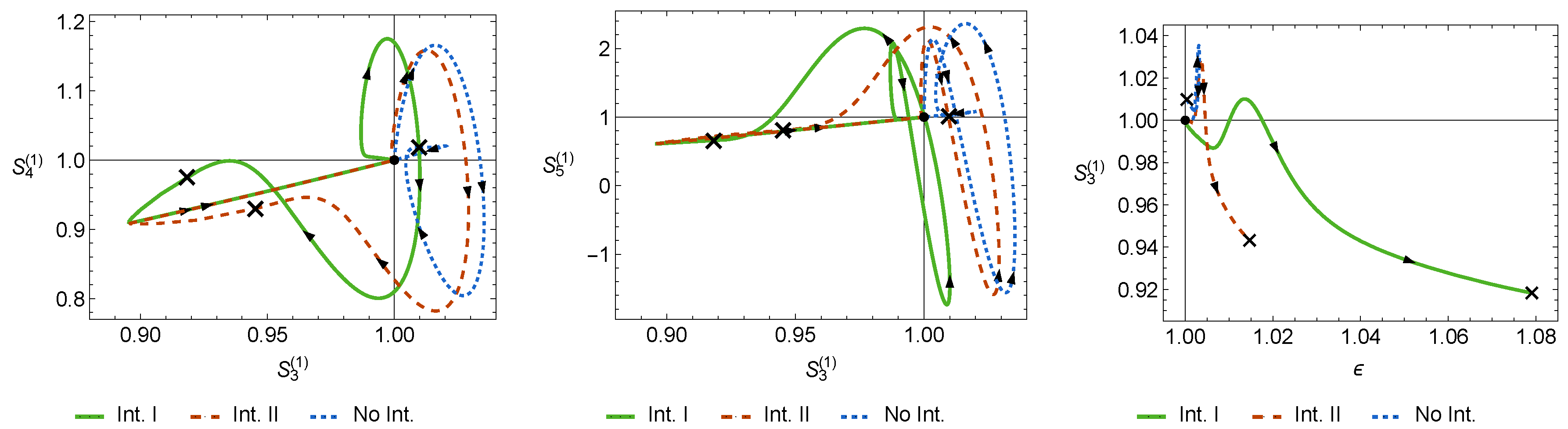
In Figure 3 we present the profiles obtained for the statefinder hierarchy and the CND of two test interactions: $Q_I=3{\alpha }_{\chi }H{\rho }_{\chi }$ and $Q_{II}=3{\alpha }_{\chi \chi }H{\rho }_{\chi }^2/({\rho }_m+{\rho }_{\chi })$ which are able to remove the LSBR in the asymptotic future and compare them with the profiles of the non-interacting model. In all three panels, a “×” symbol represents the value at the present time and the arrows indicate the direction of the time evolution. A clear distinction between the interacting and non-interacting models can be seen in the three panels: in the case of interactions I and II, the statefinder parameter ${S_3}^{\left(1\right)}$ goes well below unity, and an increase in the growth of structure $(ϵ>1)$ is observed before the Universe evolves towards the late de Sitter stage. During most of the evolution of the Universe and until the present time, the profiles of the two interacting cases can be distinguished fairly well, in particular using $\{{S_3}^{\left(1\right)};{S_4}^{\left(1\right)}\}$ and the CND.

The profiles depicted in Figure 3 were obtained by fixing the interaction parameters at ${\alpha }_{\chi }={\alpha }_{\chi \chi }=-0.03$ and the parameter of the potential at $\xi =1$. These values of the interaction parameters were chosen so as to maximise the effects of the interaction while at the same time respecting the constraints obtained in Refs. [31,32], which we took as guidelines. The evolution for each model was computed by setting the same initial conditions for all models well inside the past DM-dominated era and numerically integrating the evolution equations. The initial values of u, y, and z were chosen so that the non-interacting model better mimics ΛCDM at the present time, while ${\delta }_m$ is assumed to grow linearly with the scale factor at the initial moment. In addition, the linear perturbations of matter were obtained assuming that at all times all relevant scales are much smaller than the Hubble horizon, and that the 3-form is smooth; i.e., that its perturbations are so small that they can be disregarded [18]. We note that given these approximations, the results corresponding to $ϵ\left(x\right)$ should be considered as preliminary and with great care. A more complete approach which includes the effects of the DE perturbations and interactions at the perturbative level will be pursued in the near future.

5. Discussion

The minimally coupled massive 3-form model has been proposed in recent years as an alternative to quintessence models to explain the nature of DE [8,9]. In particular, it can naturally accommodate a phantom-like equation of state, which seems favoured by observations [5]. However, for a fairly general class of potentials that provide this behaviour, the 3-form can lead the Universe to a Little Sibling of the Big Rip event in the future (LSBR) [21]. Through a dynamical system approach, we find that the interactions between DM and the 3-form that fall in the category (9) can avoid the LSBR as long as the interaction term is not proportional to a power of the DM energy density; i.e., , with $i\ge 1$. In the case that the LSBR is successfully removed, the end state of the Universe is a de Sitter epoch with scaling behaviour between DM and the 3-form, with an almost complete 3-form domination.

To distinguish between two interactions that can remove the LSBR, we use the statefinder diagnostic $\{{S_3}^{\left(1\right)},{S_4}^{\left(1\right)}\}$, $\{{S_3}^{\left(1\right)},{S_5}^{\left(1\right)}\}$ [24] and the CND $\{ϵ,{S_3}^{\left(1\right)}\}$ [25]. Using two different interactions with similar interaction coefficients ${\alpha }_i$ as test cases, we show that both the statefinder diagnostic and the CND are adequate methods to obtain imprints that can differentiate the interacting and non-interacting models. In particular, an increase of the growth of structure is observed when the interactions are turned on, which is nevertheless within the observational constraints set by the SDSS III data [33].