Article

Cosmological Perturbations in Phantom Dark Energy Models

by
Imanol Albarran
1,2,*,
Mariam Bouhmadi-López
1,2,3,4 and
João Morais
3
1
Departamento de Física, Universidade da Beira Interior, Rua Marquês D’Ávila e Bolama, 6200-001 Covilhã, Portugal
2
Centro de Matemática e Aplicações da, Universidade da Beira Interior, Rua Marquês D’Ávila e Bolama, 6200-001 Covilhã, Portugal
3
Department of Theoretical Physics, University of the Basque Country, UPV/EHU, P.O. Box 644, 48080 Bilbao, Spain
4
Ikerbasque, Basque Foundation for Science, 48011 Bilbao, Spain
*
Author to whom correspondence should be addressed.
Universe 2017, 3(1), 22; https://doi.org/10.3390/universe3010022
Submission received: 27 January 2017 / Revised: 24 February 2017 / Accepted: 26 February 2017 / Published: 6 March 2017
(This article belongs to the Special Issue Varying Constants and Fundamental Cosmology)

Abstract

:
The ΛCDM paradigm, characterised by a constant equation of state w = 1 for dark energy, is the model that better fits observations. However, the same observations strongly support the possibility of a dark energy content where the corresponding equation of state is close to but slightly smaller than 1 . In this regard, we focus on three different models where the dark energy content is described by a perfect fluid with an equation of state w 1 which can evolve or not. The three proposals show very similar behaviour at present, while the asymptotic evolution of each model drives the Universe to different abrupt events known as (i) Big Rip; (ii) Little Rip (LR); and (iii) Little Sibling of the Big Rip. With the aim of comparing these models and finding possible imprints in their predicted matter distribution, we compute the matter power spectrum and the growth rate f σ 8 . We conclude that the model which induces a LR seems to be favoured by observations.

1. Introduction

Since the recent acceleration of the Universe was discovered by SNeIa observations around twenty years ago [1,2], and later corroborated by cosmological and astrophysical observations [3], the current acceleration of the Universe represents one of the most intriguing open problems on cosmology. Many of the models that can describe the accelerated Universe propose a new and hidden component in the Universe known as dark energy (DE) [4,5]. Alternatively, there have been attempts to amend GR in a suitable way in order to explain the recent speed-up (e.g., [6,7] and references therein).
Nowadays, the model that best fits the observational data is ΛCDM, where—apart from Cold Dark Matter (CDM)—a cosmological constant Λ is assumed. Within this framework, it is the presence of Λ with an equation of state (EoS) parameter w = 1 that drives the current acceleration of the Universe, leading it to a future de Sitter expansion. However, the tiniest deviation in the EoS parameter from this value might induce totally different fates; in particular, for values w < 1 , the Universe could face a cosmic doomsday. Curiously, this phantom-like behaviour seems to be favoured by the latest observational data [3] when the condition w = 1 is relaxed, despite the fact that it violates the null energy condition.
In this work, we have focused on three phantom DE models that can describe our current Universe, presenting only minimal deviations from ΛCDM up to the present time but which induce particular abrupt events in the future evolution of the Universe. The three events we analysed correspond to the cases that occur if and only if a phantom DE is present, and are characterised by:
i
Big Rip (BR) singularity: It happens at a finite cosmic time where the scale factor, the Hubble parameter, and its cosmic time derivatives blow up [8,9,10].
ii
Little Rip (LR): In this abrupt event, the scale factor, the Hubble parameter, and its cosmic time derivatives diverge at infinite cosmic time [11,12,13].
iii
Little Sibling of the Big Rip (LSBR): This event occurs at infinite cosmic time, where the scale factor and the Hubble parameter diverge; however, the cosmic time derivative of Hubble parameter remains finite [14,15].
Of these three scenarios, only the BR should be regarded as a true cosmological singularity, since it occurs at a finite cosmic time, while the LR and LSBR could be understood as a BR somehow driven to an infinite cosmic time; therefore, we will refer to them as abrupt events. Nonetheless, in all these cases, the Universe ends unavoidably in a classical cosmological doomsday, with all bound structures being ripped apart [12,13,14].
Here, we point out that such conclusions were based on a classical analysis of the models. However, as energy density diverges in all the cases presented, one might expect that quantum effects become important at some point in the future evolution. In fact, a quantum analysis shows that in all cases, the classical abrupt event can be avoided from a quantum point of view [16,17,18,19].
Given the serious cosmological implications of these models and their ability to mimic ΛCDM background up to the present time, we proceeded to study their profiles at first-order perturbations. Using the full linear perturbation theory, we have computed the evolution of the gravitational potentials and matter perturbations, and analysed the theoretical predictions for the matter power spectrum and growth rate f σ 8 . Other works that study the evolution of linear perturbations in doomsday scenarios with various degrees of approximation include [20,21,22], where a kinematical approach is assumed, and [23], where (like in our work) a dynamical model with a specific EoS is employed.

2. Background Models

Assuming a spatially flat Friedmann–Lemaître–Robertson–Walker (FLRW) Universe, the line element is:
d s 2 = d t 2 + a ( t ) 2 δ i j d x i d x j ,
where a ( t ) is the scale factor, t is the cosmic time, and a latin index denotes spatial coordinates. The Friedmann and Raychaudhuri equations in such Universe read
H 2 = 8 π G 3 ρ , H ˙ = 4 π G ρ + p ,
respectively. Here, H is the Hubble parameter, ρ and p the total energy density and pressure, G is the gravitational constant, and a dot stands for a derivative with respect to the cosmic time. In addition, we consider the Universe to be filled by radiation, matter, and DE, and that the conservation equation is fulfilled separately for each individual component; i.e., ρ ˙ A + 3 H ρ A + p A = 0 , where A = r , m , d representing radiation, matter, and DE, respectively. In what follows, we define for each constituent the fractional energy density, Ω A = ρ A / ρ , and EoS parameter, w A = p A / ρ A , and consider that w r = 1 / 3 and w m = 0 . Additionally, a 0-subscript denotes the present value of a given quantity, and we set a 0 = 1 .
We now introduce the three models studied in this work. In each case, we present an equation of state that leads to the corresponding abrupt event in the future, as well as the evolution of ρ d a , which was obtained by solving the conservation equation:
i
The BR singularity model: a singularity of the type BR [8,9,10] can be induced by a perfect fluid whose EoS parameter is constant and smaller than 1 .
p d = w d ρ d , ρ d a = ρ d 0 a 3 1 + w d , w d < 1 .
The values of the free parameters for this model are taken from the Planck data for wCDM model [24]: w d = 1.019 , Ω m 0 = 0.306 and H 0 = 68.1 Km · Mpc 1 · s 1 (cf. page 687 of [24]).
ii
The LR abrupt event model: an event of the type LR [11,12,13] can be caused by a perfect fluid whose EoS and energy density can be written as [12]
p d = ρ d + B ρ d 1 / 2 , ρ d a = ρ d 0 3 2 Ω d 0 Ω * ln a a 0 + 1 2 , B > 0 ,
where Ω * 8 π G B 2 / ( 3 H 0 2 ) . In order to fix the free parameters of this model, we use the results obtained in [12], where the authors use the data given by the Supernova Cosmology Project [25,26] to constrain the parameters: Ω m 0 = 0.274 , H 0 = 70.1 Km · Mpc 1 · s 1 , and Ω * = 7.7637 × 10 4 .
iii
The LSBR abrupt event model: the event denominated as LSBR can be induced by a perfect fluid whose EoS deviates from that of a cosmological constant by adding a constant parameter [14]. Therefore, the corresponding EoS and energy density in terms of the scale factor can be written as
p d = ρ d + A 3 , ρ d a = ρ d 0 + A ln a a 0 , A > 0 .
Note that ρ d 0 plays the role of a cosmological constant. In this case, we have chosen the numerical value taken in [14]: A = 10 3 3 H 0 2 / 8 π G , while for Ω m 0 and H 0 , we have used the same values as in the case for the BR.

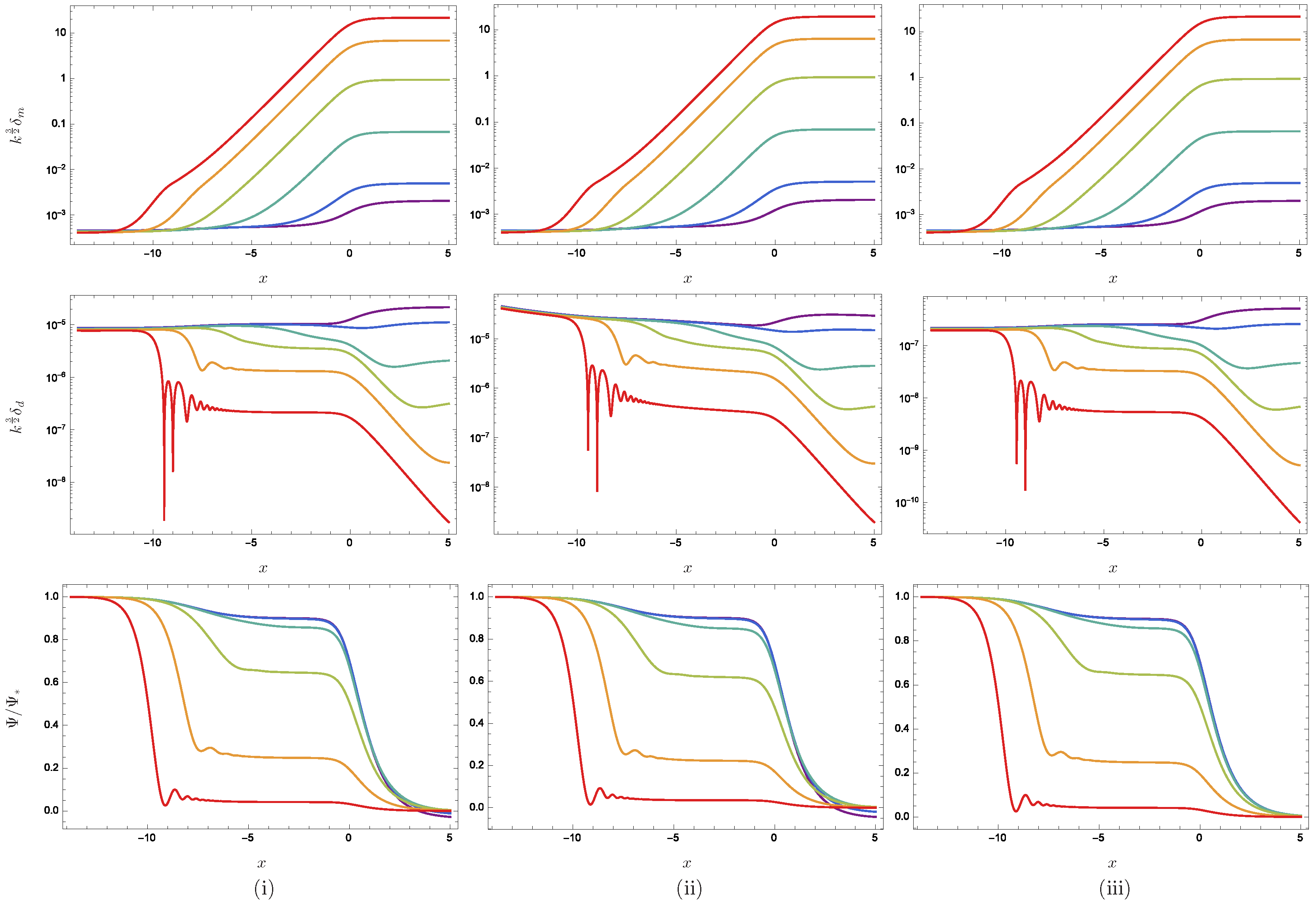
3. Perturbed Equations
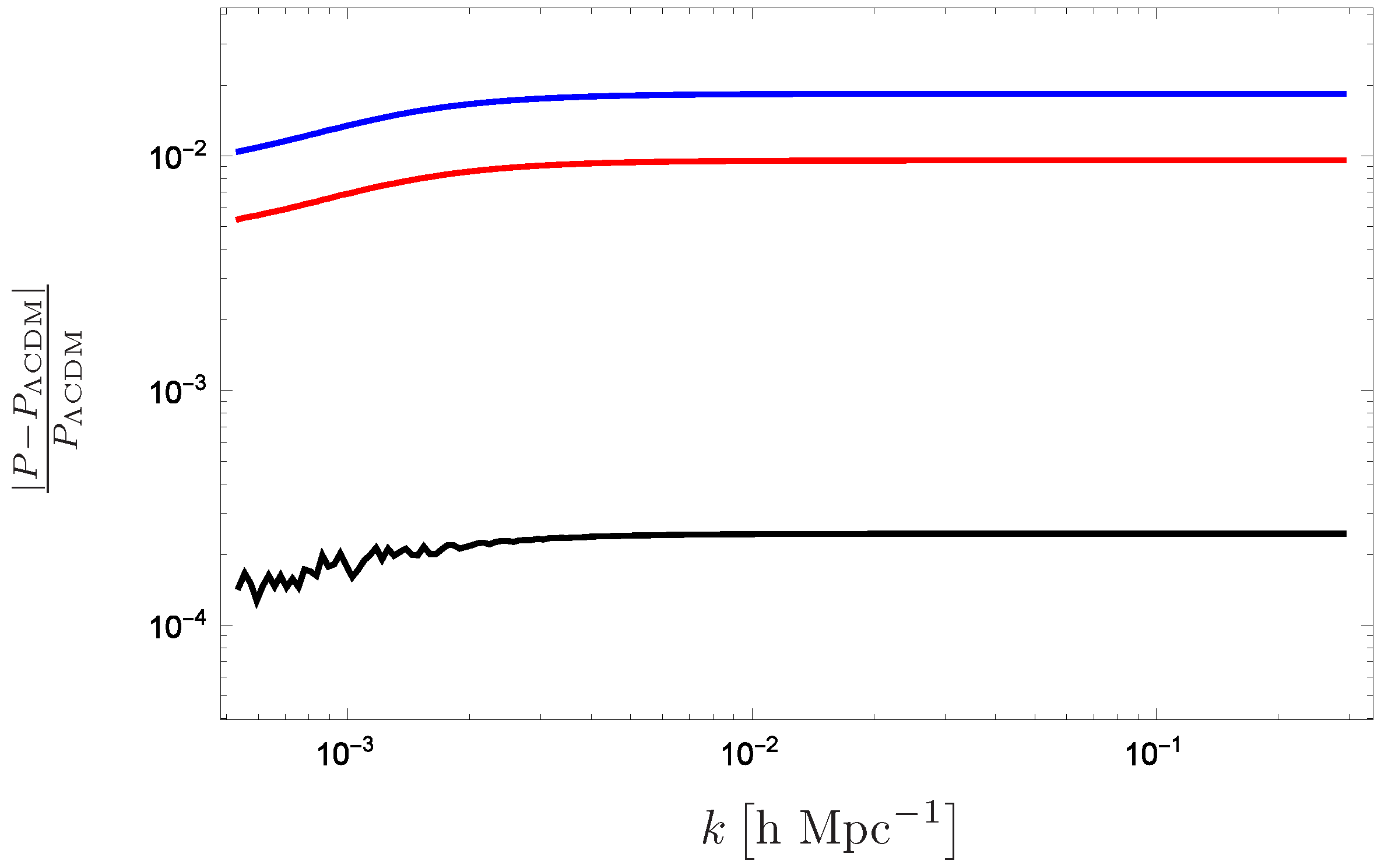
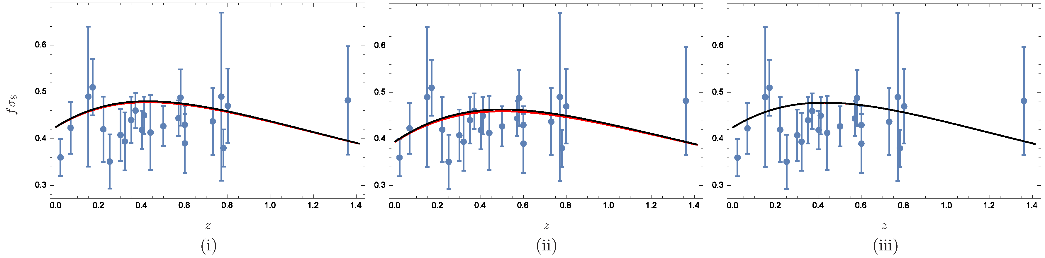
In the Newtonian gauge, the FLRW perturbed line element is [27]
d s 2 = a 2 1 + 2 Φ d η 2 + 1 2 Ψ δ i j d x i d x j ,
where η is the comoving time defined as d η = ( 1 / a ) d t , and Ψ ( η , x i ) and Φ ( η , x i ) are the gauge-invariant Bardeen potentials [28]1. For each fluid, the individual components of the perturbed energy momentum tensor, δ T A ν μ , read
δ T A 0 0 = δ ρ A , δ T A 0 i = δ T A i 0 = p + ρ i v A , δ T A j i = δ p A δ j i ,
where δ ρ A is the energy density perturbation, δ p A is the pressure perturbation, and v A is the velocity potential. Following [29,30], we decompose the pressure perturbation as
δ p A = c s A 2 δ ρ A 3 H 1 + w A c s A 2 c a A 2 ρ A v A .
where H = a / η / a is the comoving Hubble rate, c s A 2 = δ p A / δ ρ A r . f . is the effective speed of sound in the rest frame (r.f.), and c a A 2 = p ˙ A / ρ ˙ A is the adiabatic speed of sound where A stands for the radiation, matter, and DE perturbations. While we consider both radiation and matter as adiabatic fluids ( c s A 2 = c a A 2 ), for DE we take c s A 2 = 1 in order to avoid the instabilities related with imaginary values of the speed of sound [29]. Implicit in this choice is the assumption that the EoS of the three models is an effective description of a more fundamental and unknown matter description.
In Fourier space, the evolution equations of the perturbations of the three fluids 2 can be obtained from the perturbed conservation equations, and read
δ r x = 4 3 k 2 H v r + 3 Ψ x , v r x = 1 H 1 4 δ r + Ψ ,
δ m x = k 2 H v r + 3 Ψ x , v m x = v m + Ψ H ,
δ d x = 1 + w d k 2 H + 9 H 1 c a d 2 v d + 3 Ψ x + 3 w d 1 δ d , v d x = 1 H 1 1 + w d δ d + Ψ + 2 v d ,
where k is the wave-number and a subscript x indicates a derivative with respect to x ln a / a 0 . Using the perturbed Einstein equations, we can relate the metric potential and its derivative with the energy density perturbations and the peculiar velocities
Ψ x + 1 + k 2 3 H 2 Ψ = 1 2 Ω A δ A , Ψ x + Ψ = 3 2 H Ω A 1 + w A v A .
In order to obtain the imprints of each model at the perturbative level, Equations (9)–(11)—in combination with Equation (12)—need to be integrated numerically. The initial conditions for such integration are obtained by considering that—initially—the Universe is well inside the radiation epoch ( a / a 0 = 10 6 ) with all the relevant modes inside the Hubble horizon ( k H ). In this regime, the gravitational potential is constant, Ψ x = 0 , which in conjunction with initial adiabatic conditions leads to [5,31]
δ r 1 + w r = δ m 1 + w m = δ d 1 + w d = δ 1 + w , v r = v m = v d δ 4 H .
Here, δ is the total fractional energy density perturbation and the total EoS parameter is assumed to be w 1 / 3 in the radiation epoch. From Equation (13), we find that all the initial conditions to be defined in terms of the initial value of δ. Using single field inflation standard results, we find [3]
δ ( k ) = 8 π 3 2 A s k k * n s 1 2 k 3 2 ,
where A s = 2.143 × 10 9 and n s = 0.9681 are the observational values of the amplitude and spectral index of the primordial inflationary power spectrum corresponding to the pivot scale k * = 0.05 Mpc 1 [3].

4. Results

In Figure 1, we present the evolution of the perturbations δ m , δ d , and Ψ from the radiation epoch ( x 13.81 , which corresponds to a / a 0 = 10 6 ) until the future time ( x = 5 ) for different wave-numbers k ranging from k = 3.33 × 10 4 h · Mpc 1 (purple) to k = 0.30 h · Mpc 1 (red). The first and second row represent , respectively, the evolution of fractional energy density corresponding to DM, δ m , and DE, δ d , while the third row presents the evolution of the gravitational potential. Finally, the results for the three studied models are separated by columns, where the first, second, and third columns correspond to the model (i), the model (ii) and the model (iii), respectively.
As can be seen in the first row of Figure 1, the evolution of the matter perturbations for different models are almost indistinguishable among them. At the initial radiation-dominated epoch, all modes remain constant until they enter their Hubble horizon; then, during the matter-dominated epoch, the growth of δ m becomes exponential on x. Finally, when DE dominates over the other components, the growth of the matter perturbations reach a constant value.
Similarly, in the DE perturbations, the evolution of each mode is quite similar for the three models; the exception in this case lies on the amplitude of δ d , where the amplitude can be up to two orders of magnitude. These deviations do not depend on the wave-number, but on the value of the corresponding w d at the beginning, where the tiniest deviation from 1 can induce large variations in the initial conditions (13) which are propagated over the whole evolution.
The third row of Figure 1 shows the evolution of the normalised gravitational potential Ψ / Ψ * , where Ψ * corresponds to the initial value of Ψ. Once again, the models exhibit almost indistinguishable behaviours without any particular imprint. During the initial radiation-dominated epoch, all the modes start with a constant value, then decay during the matter era to finally vanish when DE totally dominates the future.
As we have shown, the models studied in this work show very similar behaviours; consequently, the matter power spectrum predicted by each model is almost indistinguishable. In order to give an account of the difference between the models, we have computed the relative deviation of the matter power spectrum in comparison with the ΛCDM model.
Using the results of the numerical integration, we were able to determine the theoretical prediction for the matter power spectrum, P δ ^ m , which is defined in the comoving gauge as P δ ^ m = | δ m ( c o m ) | 2 = δ m 3 H v m 2 .
In Figure 2, we present the relative deviation of the power spectrum of each model with respect to the predictions of ΛCDM. As can be seen, the difference remains constant for almost all modes, and decreases for very small wave-numbers. Model (i) shows the largest difference (less than 0.02 ), while model (iii) deviates less from ΛCDM. Notice that model (iii) has not been observationally constrained, and we took suitable values for the model parameter in order to deviate as little as possible from ΛCDM in the past.
Finally, we have obtained the observational quantity f σ 8 , where f = ( 1 / δ m ) ( δ m / x ) is the growth rate of structure and σ 8 is the root mean square mass fluctuation amplitude in spheres of radius 8 h 1 · Mpc , which is used to normalise the matter power spectrum [32]. The theoretical prediction of f σ 8 can be computed as
f σ 8 ( x ) = σ 8 0 , k σ 8 δ m x , k σ 8 δ m 0 , k σ 8 d ln δ m d x .
In Figure 3, we present the evolution of f σ 8 for the three models (black curve) and the corresponding ΛCDM model (red curve) against several observational points in the range z ( 0 , 1.4 ) , ( please, see [33] and references therein).
As can be seen, all models are within the error bars for practically all the points and show almost indistinguishable behaviour in comparison with the ΛCDM model. In order to quantify the deviation between the theoretical prediction and observational data, we compute the value of χ 2 for each model [33], and we find the following results: χ 2 ( i ) = 27.63 , χ 2 ( i i ) = 16.53 , and χ 2 ( i i i ) = 26.30 . Model (ii) has the smaller χ 2 , while models (i) and (iii) have higher but similar values; consequently, we can argue that model (ii) is favoured by observations. The high tension between the theoretical predictions and the data in models (i) and (iii) seems to come from the fact that we used Planck data for those models, which have a higher value of Ω m 0 than the Supernova Cosmology Project data used for model (ii).

5. Discussion

In this work, we analyse the cosmological perturbations for three possible phantom DE scenarios where each of them induces a unique future abrupt event: Big Rip (BR), Little Rip (LR), and Little Sibling of the Big Rip (LSBR). Despite their catastrophic implications for the future of the Universe, each of these models present small deviations from the widely-accepted ΛCDM model, and therefore could scope the current observational constraints. After numerically computing the evolution of all perturbed quantities (the integrations are performed from well inside the radiation era until the far future), we compare the results for each model by looking at the profile of the gravitational potential Ψ, the perturbations of DM (which grow linearly during the matter era), and the DE perturbations, which remain small during the whole history of the Universe (cf. Figure 1). We find that the theoretical outcomes given for each model are very similar to each other—in particular for δ m and δ d . While each model leaves some identifying imprints on δ d , in practice, the small amplitude of the perturbations weakens them as identifiers of the model. In order to look for observational fingerprints of the models, we compute the matter power spectrum at present, which we compare with the one of ΛCDM (Figure 2), and the evolution of f σ 8 , which we compare with ΛCDM predictions and the observational data points at low redshift ( z < 1.4 ) (Figure 3). We find that for all models, the deviations from the ΛCDM results are 2 % , and that model (iii)—which induces the LSBR—presents less deviations from ΛCDM at the level of the matter power spectrum. However, this result must be taken carefully, considering that the parameter A was not constrained observationally; instead, its value was chosen to deviate as little as possible from the ΛCDM at the present. For f σ 8 we, once again find a great similarity between the studied models and ΛCDM. However, a χ 2 analysis shows that model (ii)—which induces an LR event—is the most favoured by observations.
We conclude that the obtained results are in agreement with the observational data, and therefore, even if ΛCDM model gives the best fit, there is no reason to exclude these models that can suitably describe the current Universe. However, we stress that as we did not make an observational fit of these models at the background level, all our results should be taken as a guideline for a more accurate study that we hope to carry out in the future.

Acknowledgments

The work of I.A. was supported by a Santander-Totta fellowship “Bolsas de Investigação Faculdade de Ciências (UBI) -Santander Totta”. The work of M.B.-L. is supported by the Portuguese Agency “Fundação para a Ciência e Tecnologia” through an Investigador FCT Research contract, with reference IF/01442/2013/CP1196/CT0001. She also wishes to acknowledge the partial support from the Basque government Grant No. IT592-13 (Spain) and FONDOS FEDER under grant FIS2014-57956-P (Spanish government). This research work is partially supported by the grant UID/MAT/00212/2013. J.M. is thankful to UPV/EHU for a PhD fellowship and acknowledges the support from the Basque government Grant No. IT592-13 (Spain) and FONDOS FEDER, under grant FIS2014-57956-P (Spanish Government). The authors acknowledge the COST Action CA15117 (CANTATA).

Author Contributions

The authors contributed equally to this paper.

Conflicts of Interest

The authors declare no conflict of interest.

References

  1. Riess, A.G.; Filippenko, A.V.; Challis, P.; Clocchiatti, A.; Diercks, A.; Garnavich, P.M.; Gilliland, R.L.; Hogan, C.J.; Jha, S.; Kirshner, R.P.; et al. Observational Evidence from Supernovae for an Accelerating Universe and a Cosmological Constant. Astrophys. J. 1998, 116, 1009–1038. [Google Scholar] [CrossRef]
  2. Perlmutter, S. Supernova Cosmology Project Collaboration. Astrophys. J. 1999, 517, 565–586. [Google Scholar] [CrossRef]
  3. Ade, P.A.; Aghanim, N.; Arnaud, M.; Ashdown, M.; Aumont, J.; Baccigalupi, C.; Banday, A.J.; Barreiro, R.B.; Bartlett, J.G.; Bartolo, N.; et al. Planck 2015 results. XIII. Cosmological parameters. Astron. Astrophys. 2015, 594, A13. [Google Scholar]
  4. Bamba, K.; Capozziello, S.; Nojiri, S.I.; Odintsov, S.D. Dark energy cosmology: The equivalent description via different theoretical models and cosmography tests. Astrophys. Space Sci. 2012, 342, 155–228. [Google Scholar] [CrossRef]
  5. Amendola, L.; Tsujikawa, S. Dark Energy: Theory and Observations, 1st ed.; Cambridge University Press: Cambridge, UK, 2010. [Google Scholar]
  6. Capozziello, S.; Faraoni, V. Beyond Einstein Gravity: A Survey of Gravitational Theories for Cosmology and Astrophysics; Springer Science & Business Media: New York, NY, USA, 2011; Volume 170. [Google Scholar]
  7. Morais, J.; Bouhmadi-López, M.; Capozziello, S. Can f (R) gravity contribute to (dark) radiation? J. Cosmol. Astropart. Phys. 2015, 2015, 41. [Google Scholar] [CrossRef]
  8. Starobinsky, A.A. Future and origin of our universe: Modern view. Grav. Cosmol. 2000, 6, 157–163. [Google Scholar]
  9. Carroll, S.M.; Hoffman, M.; Trodden, M. Can the dark energy equation-of-state parameter w be less than -1? Phys. Rev. D 2003, 68, 023509. [Google Scholar] [CrossRef]
  10. González-Díaz, P.F. K-essential phantom energy: Doomsday around the corner? Phys. Lett. B 2003, 586, 1–4. [Google Scholar] [CrossRef]
  11. Ruzmaikina, T.; Ruzmaikin, A.A. Quadratic corrections to the Lagrangian density of the gravitational field and the singularity. Sov. Phys. JETP 1970, 30, 372. [Google Scholar]
  12. Frampton, P.H.; Ludwick, K.J.; Scherrer, R.J. The Little Rip. Phys. Rev. D 2011, 84, 063003. [Google Scholar] [CrossRef]
  13. Frampton, P.H.; Ludwick, K.J.; Nojiri, S.; Odintsov, S.D.; Scherrer, R.J. Models for Little Rip Dark Energy. Phys. Lett. B 2012, 708, 204–211. [Google Scholar] [CrossRef]
  14. Bouhmadi-López, M.; Errahmani, A.; Martín-Moruno, P.; Ouali, T.; Tavakoli, Y. The little sibling of the big rip singularity. Int. J. Mod. Phys. D 2015, 24, 1550078. [Google Scholar] [CrossRef]
  15. Morais, J.; Bouhmadi-López, M.; Sravan Kumar, K.; Marto, J.; Tavakoli, Y. Interacting 3-form dark energy models: Distinguishing interactions and avoiding the Little Sibling of the Big Rip. Phys. Dark Universe 2017, 15, 7–30. [Google Scholar] [CrossRef]
  16. Da̧browski, M.P.; Kiefer, C.; Sandhöfer, B. Quantum phantom cosmology. Phys. Rev. D 2006, 74, 044022. [Google Scholar] [CrossRef]
  17. Albarran, I.; Bouhmadi-López, M. Quantisation of the holographic Ricci dark energy model. J. Cosmol. Astropart. Phys. 2015, 2015, 51. [Google Scholar] [CrossRef]
  18. Albarran, I.; Bouhmadi-López, M.; Cabral, F.; Martín-Moruno, P. The quantum realm of the “Little Sibling” of the Big Rip singularity. J. Cosmol. Astropart. Phys. 2015, 2015, 44. [Google Scholar] [CrossRef]
  19. Albarran, I.; Bouhmadi-López, M.; Kiefer, C.; Marto, J.; Vargas Moniz, P. Classical and quantum cosmology of the little rip abrupt event. Phys. Rev. D 2016, 94, 063536. [Google Scholar] [CrossRef]
  20. Balcerzak, A.; Denkiewicz, T. Density preturbations in a finite scale factor singularity universe. Phys. Rev. D 2012, 86, 023522. [Google Scholar] [CrossRef]
  21. Denkiewicz, T. Dark energy and dark matter perturbations in singular universes. J. Cosmol. Astropart. Phys. 2015, 2015, 37. [Google Scholar] [CrossRef]
  22. Denkiewicz, T. Dynamical dark energy models with singularities in the view of the forthcoming results of the growth observations. arXiv 2015. [Google Scholar]
  23. Astashenok, A.V.; Odintsov, S.D. Confronting dark energy models mimicking ΛCDM epoch with observational constraints: Future cosmological perturbations decay or future Rip? Phys. Lett. B 2013, 718, 1194–1202. [Google Scholar] [CrossRef]
  24. Planck 2015 Results: Cosmological Parameter Tables. Available online: https://wiki.cosmos.esa.int/planckpla2015/images/0/07/Params_table_2015_limit95.pdf (accessed on 28 February 2017).
  25. WMAP Cosmological Parameters. Available online: http://lambda.gsfc.nasa.gov/product/map/dr4/params/lcdm_sz_lens_wmap7_bao_h0.cfm (accessed on 28 February 2017).
  26. Amanullah, R.; Lidman, C.; Rubin, D.; Aldering, G.; Astier, P.; Barbary, K.; Burns, M.S.; Conley, A.; Dawson, K.S.; Deustua, S.E.; et al. Spectra and Light Curves of Six Type Ia Supernovae at 0.511 < z < 1.12 and the Union2 Compilation (The Supernova Cosmology Project). Astrophys. J. 2010, 716, 712–738. [Google Scholar]
  27. Kurki-Suonio, H. Cosmological Perturbation Theory; Lecture Notes; University of Helsinki: Helsinki, Finland, 2003. [Google Scholar]
  28. Bardeen, J.M. Gauge-invariant cosmological perturbations. Phys. Rev. D 1980, 22, 1882. [Google Scholar] [CrossRef]
  29. Bean, R.; Dore, O. Probing dark energy perturbations: The Dark energy equation of state and speed of sound as measured by WMAP. Phys. Rev. D 2004, 69, 083503. [Google Scholar] [CrossRef]
  30. Väliviita, J.; Majerotto, E.; Maartens, R. Large-scale instability in interacting dark energy and dark matter fluids. J. Cosmol. Astropart. Phys. 2008, 2008, 20. [Google Scholar] [CrossRef] [Green Version]
  31. Ballesteros, G.; Lesgourgues, J. Dark energy with non-adiabatic sound speed: Initial conditions and detectability. J. Cosmol. Astropart. Phys. 2010, 2010, 14. [Google Scholar] [CrossRef]
  32. Wang, Y.; Percival, W.; Cimatti, A.; Mukherjee, P.; Guzzo, L.; Baugh, C.M.; Carbone, C.; Franzetti, P.; Garilli, B.; Geach, J.E.; et al. Designing a space-based galaxy redshift survey to probe dark energy. Mon. Not. R. Astron. Soc. 2010, 409, 737–749. [Google Scholar] [CrossRef] [Green Version]
  33. Albarran, I.; Bouhmadi-López, M.; Morais, J. Cosmological perturbations in an effective and genuinely phantom dark energy Universe. arXiv 2016. [Google Scholar]
  • 1.In this work we disregard any anisotropy at the linear level of the scalar perturbations, therefore, from this point onward we will set Ψ = Φ [27].
  • 2.From now on, all perturbed quantities referred to in the manuscript represent the Fourier transform action of such perturbations, even though no specific notation is used, e.g., Ψ = Ψ ( x , k ) , where k is the wave-number.
Figure 1. The first, second, and third row of this figure presents the evolution of dark matter (DM), dark energy (DE), and the gravitational potential perturbations, respectively. Each column belongs to a particular model, while each colour represents a mode where the values of the corresponding wave-number are: k = 3.33 × 10 4 h · Mpc 1 (purple); k = 7.93 × 10 4 h · Mpc 1 (dark blue); k = 3.50 × 10 3 h · Mpc 1 (light blue); k = 1.54 × 10 2 h · Mpc 1 (green); k = 6.80 × 10 2 h · Mpc 1 (orange); k = 0.30 h · Mpc 1 (red).
Universe 03 00022 g001
Figure 2. The relative deviation of the matter power spectrum of: model (i) in red; model (ii) in blue; and model (iii) in black; with regards to the predictions of ΛCDM (CDM: cold dark matter). The model that induces a Big Rip (BR) singularity shows the highest deviation, while the model that induces a Little Sibling of the Big Rip (LSBR) abrupt event presents the smallest deviation with respect to the ΛCDM model.
Universe 03 00022 g002
Figure 3. The evolution of f σ 8 in terms of the redshift for each model (black curve) together with the corresponding ΛCDM model (red curve). The blue dots and corresponding error bars indicate observational values ( please, see [33] and references therein).
Universe 03 00022 g003

