
The Relation between Fundamental Constants and Particle Physics Parameters

Steward Observatory and Department of Astronomy, University of Arizona, Tucson, AZ 85721, USA
Universe 2017, 3(1), 6; https://doi.org/10.3390/universe3010006
Submission received: 16 December 2016
/
Revised: 12 January 2017
/
Accepted: 13 January 2017
/
Published: 24 January 2017
(This article belongs to the Special Issue Varying Constants and Fundamental Cosmology)
Abstract
:The observed constraints on the variability of the proton to electron mass ratio μ and the fine structure constant α are used to establish constraints on the variability of the Quantum Chromodynamic Scale and a combination of the Higgs Vacuum Expectation Value and the Yukawa couplings. Further model dependent assumptions provide constraints on the Higgs VEV and the Yukawa couplings separately. A primary conclusion is that limits on the variability of dimensionless fundamental constants such as μ and α provide important constraints on the parameter space of new physics and cosmologies.
1. Introduction
Over the past two decades, there has been a renewed interest in measuring fundamental dimensionless constants such as the proton to electron mass ratio μ and the fine structure constant α in the early universe. Modulo some possibilities discussed at this conference, impressive constraints on the variation of μ and α have been established over time periods that span a significant fraction of the age of the universe. Here, the implications of those constraints are examined in terms of the stability of three basic physics parameters: the Quantum Chromodynamic Scale , the Higgs Vacuum Expectation Value ν and the Yukawa Couplings h. Previous reports of a possible variation of α [1] spurred significant efforts to account for the variation in terms of varying , ν and h [2,3,4,5,6,7,8,9,10]. These efforts form the basis of the present work except that the process is reversed in that constraints on the variability of the physics parameters is established in terms of the limits on the variability of μ and α. Most of the earlier efforts limited the variability to only one of the physics parameters, usually . In contrast, the work of [5] considered the possibility of all three parameters varying. As such, it is the primary reference in this work.
2. Observational Constraints
There are relatively few constraints on the variation of μ since molecular spectra provide the primary limits on the variability of μ [11] and only a few molecular spectra at high redshift exist. On the other hand, radio observations of molecular spectra at moderate redshifts provide a significantly tighter constraint on μ than exists for α. The current limits on both μ and α are given below.
2.1. Constraints
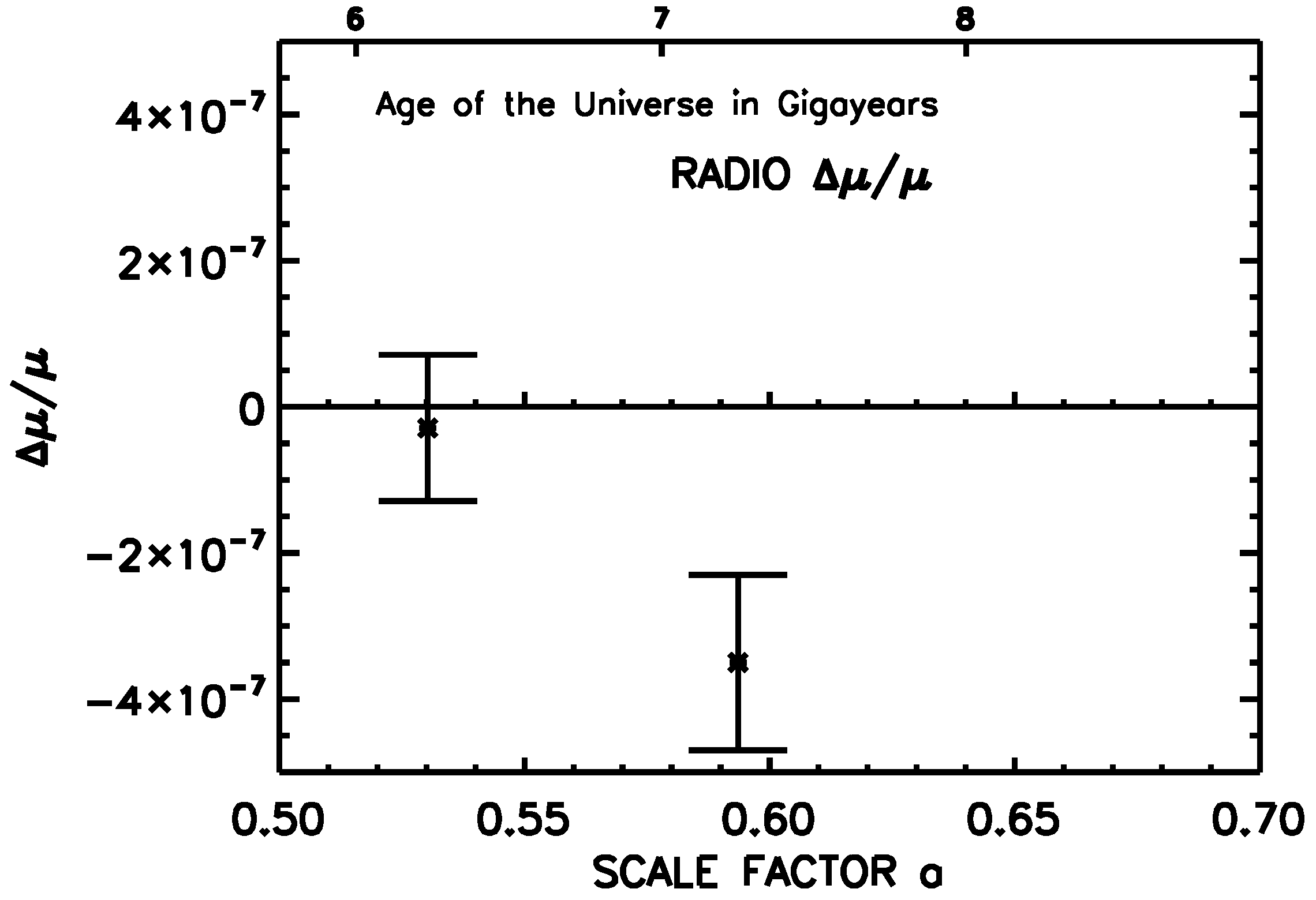
The constraints on come from optical observations of redshifted electronic transitions of molecular hydrogen and from radio observations of methanol and ammonia molecules. The majority of the observations are at redshifts greater than two where the ultraviolet rest frame transitions enter the optical bands and the current radio observations are all at redshifts less than one. The radio observations, however, are significantly more accurate than the optical observations. The radio observations of methanol in PKS1830-211 [12] at a redshift of 0.88582 is currently the tightest constraint on a variation of μ. In spite of the relatively low redshift, the look back time is greater than half the age of the universe. Figure 1 and Table 1 show all of the constraints on the variation of μ with error bars. The radio observations are shown separately in Figure 2 since they are barely visible in Figure 1.
2.2. α Constraints
Contrary to the case with μ, there are several thousand measurement of the fine structure splitting at many redshifts of which several hundred are appropriate for testing for a variation of α. In two cases [1,23], temporal changes in α are reported with [23] reporting both spatial and temporal changes at the level. (See the contributions by Webb et al. in these proceedings.) Subsequent work by [24], however, sees no variation at the at the level where the error is the rms of the statistical and systematic errors. This is a significantly lower constraint than the reported variation by [23] of ≈ and consistent with no change in α. Reference [24] attributes the difference to known wavelength calibration errors in the previous analysis in [1,23]. For the purposes of this work, the limits on a variation of α discussed in [24] are taken as the primary limit.
3. The Dependence of Fundamental Constants on the Physics Parameters
The numerical values of both α and μ depend on the values of the physics parameters , ν and h. The following follows the discussion of [5] done for a different purpose but relevant to the current analysis. The connection between the fundamental constants and the physics parameters is probably most obvious for the proton to electron mass ratio μ where the physics parameters set the mass of the proton and electron.
3.1. The Proton to Electron Mass Ratio
The fractional change of μ, by simple mathematics is
The fractional change of the electron mass is easy since it is a fundamental particle whose mass is set by the Higgs VEV and the electron Yukawa coupling such that , therefore
The mass of the proton, however, is much more complicated since it is a composite particle but the fractional change is easier since the ratio eliminates some of the terms. In [5], the fractional change of the proton mass is given by
Both a and b are scalars of order unity whose sum by dimensional requirements should equal one to ensure that the proton has units of mass. Combining (2) and (3) gives
Here, the common assumption that although the Yukawa couplings have different values their fractional changes should be the same is employed. Next, using b is eliminated and the fractional change of μ is
3.2. The Fine Structure Constant
Without additional information, (5) only constrains the combination of , ν, and h rather than any of them individually. The observational constraints on can provide some of that information since it constrains a different combination of the three parameters. From [5] depends on the three parameters as
A new model dependent parameter R is introduced that can range between unity and in excess of 100. In [5], R is taken as 36 based on unification arguments. For the purposes of this work, that value is accepted partially since it is in the midrange of currently acceptable values. Both (5) and (6) effectively depend on two variables, and which provides a mechanism for solving for as a function of the constraints on the variance of μ and α and the model dependent parameters.
The Physics of R
Various authors use different models and assumptions to set the value of R. An example is [7] who assumes that the variation in α is produced by temporal changes of the GUT unification scale which also makes the physics parameters time variable. In this model R is given by
where the are the beta function coefficients that scale . At the unification scale all of the beta functions are unified to . is defined as . The different gauge couplings are then given by
The GUT scale is allowed to change but and are held constant where is the Planck mass. At the unification scale, R is given by
As becomes either positively or negatively large, the value of R approaches 36, the value used in [5].
4. Observational Constraints on
The combination of constraints on the fractional variation of two fundamental constants μ and α provides the opportunity to put constraints on the fractional variation of . Eliminating from (5) and (6) yields
where both factors a and b from (3) have been retained. In [5] and . Again invoking (10) simplifies to
Eliminating provides a constraint on of
Individual Constraints on and
At the expense of additional model dependence, it is possible to individually constrain and . In the standard model, there is an established relationship between the fractional variation of the Higgs VEV ν and the fractional variation of the Yukawa couplings h given by [5].
The value of S is model dependent so the constraints on and are doubly model dependent. These constraints come from using (13) in (12). The ± in the and terms in Equations (14) and (15) simply reflect that limits on and are plus or minus the quoted error. As stated in Section 5, the terms are combined as a root mean square when evaluated.
Similarly the limit on is
5. Constraints from a Given Model
Since the discussion has followed the work of [5], the model used in that reference is used as an example for producing constraints on the physics parameters. It is also a constraint on the particular model as well. The values for the model dependent parameters in [5] are , (which add to one), and . Note that with this parameter set and the observational constraints, the common leading term, the α term, in (11) and (12) dominate the constraints on the parameters. The constraints are
The look back time for the constraints is the average look back time of the α observations at a redshift of 1.54 equal to 9.4 gigayears or roughly of the age of the universe.
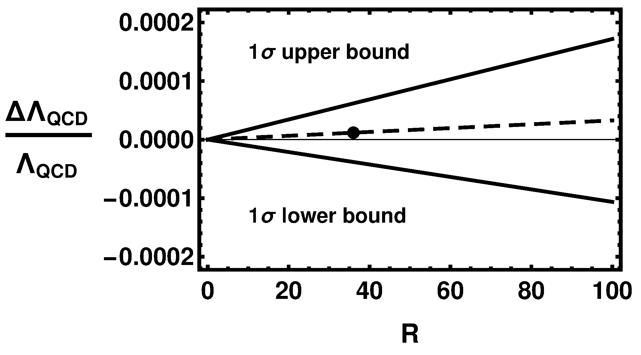
The observational constraints are evaluated via rms summing of the α and μ terms for each parameter. This assumes that the errors are centered on zero rather than the “measured” values of the observations. It was noted earlier that the R model parameter has a range of model values. Figure 3 shows the variation of the limit on as a function of R.
6. A Model Dependent Limit on
The observational constraints on the physics parameters are dominated by the α term both because of its less stringent observational limit and by the larger coefficient in the model of [5]. That model, however, predicts a relationship between a variation of α and a variation of μ given by
The model therefore predicts that the fractional variation of α should be smaller than the variation of μ by a factor of 1/36. It is of some interest to see how the constraints on the physics parameters change if this model dependent limit of on the fractional change of α is imposed. The new constraint on is
The net result of the model dependent limit on is a very stringent set of limits on the fractional change of the parameters at the look back time of the μ constraints which is greater than half the age of the universe. This constraint severely limits the parameter space of theories that predict significant fractional changes in , ν or h.
7. Conclusions
It is difficult to test for time variability of the primary particle physics parameters such as the Quantum Chromodynamic Scale, the Higgs Vacuum Expectation Value and the Yukawa couplings. It is, however, relatively easy to use spectra of objects in the early universe to test for time variability of dimensionless fundamental constants whose numerical values depend on the physics parameters. Individually, the constants only constrain a combination of the parameters but combining the observational constraints on the variability of two or more constants provides model dependent constraints on the fractional variability of the QCD scale and a combination of the fractional variability of the Higgs VEV and the Yukawa couplings. Introduction of an additional model dependent parameter sets limits on the fractional variability of the Higgs VEV and the Yukawa couplings separately.
The constraints on the fractional time variability of the physics parameters limits the parameter space of new physics theories that require a time variability of any of the three basic physics parameters. It is recommended that observed constraints on the variability of dimensionless fundamental constants become another important tool in evaluating the validity of non-standard physics and cosmology theories.
Conflicts of Interest
The author declares no conflict of interest.
References
- Webb, J.K.; Murphy, M.T.; Flambaum, V.V.; Dzuba, V.A.; Barrow, J.D.; Churchill, C.W.; Prochaska, J.X.; Wolfe, A.M. Further Evidence for Cosmological Evolution of the Fine Structure Constant. Phys. Rev. Lett. 2001, 87, 091301. [Google Scholar] [CrossRef] [PubMed]
- Calmet, X.; Fritzsch, H. Symmetry Breaking and Time Variation of Gauge Couplings. Phys. Lett. B 2002, 540, 173–178. [Google Scholar] [CrossRef]
- Campbell, B.A.; Olive, K.A. Nucleosynthesis and the time dependence of fundamental couplings. Phys. Lett. B 1995, 345, 429–434. [Google Scholar] [CrossRef]
- Chamoun, N.; Landou, S.J.; Mosquera, M.E.; Vucetich, H. Helium and deuterium abundances as a test for the time variation of the fine structure constant and the Higgs vacuum expectation value. J. Phys. G Nucl. Part. Phys. 2007, 34, 163–176. [Google Scholar] [CrossRef]
- Coc, A.; Nunes, N.J.; Olive, K.A.; Uzan, J.-P.; Vangioni, E. Coupled variations of fundamental couplings and primordial nucleosynthesis. Phys. Rev. D 2007, 76, 023511. [Google Scholar] [CrossRef]
- Dent, T. Fundamental constants and their variability in theories of High Energy Physics. Eur. Phys. J. Spec. Top. 2008, 163, 297–313. [Google Scholar] [CrossRef]
- Dine, M.; Nir, Y.; Raz, G.; Volansky, T. Time variations in the scale of grand unification. Phys. Rev. D 2003, 67, 015009. [Google Scholar] [CrossRef]
- Langacker, P.; Segre, G.; Strassler, M.J. Implications of gauge unification for time variation of the fine structure constant. Phys. Lett. B 2002, 528, 121–128. [Google Scholar] [CrossRef]
- Langacker, P. Time Variation of Fundamental Constants as a Probe of New Physics. Int. J. Mod. Phys. A 2004, 19, 157–165. [Google Scholar] [CrossRef]
- Uzan, J.-P. Varying constants, Gravitation and Cosmology. Living Rev. Relativ. 2011, 14, 2. [Google Scholar] [CrossRef]
- Thompson, R.I. The Determination of the Electron to Proton Inertial Mass Ratio via Molecular Transitions. Astrophys. Lett. 1975, 15, 3–4. [Google Scholar]
- Kanekar, N.; Ubachs, W.; Menten, K.M.; Bagdonaite, J.; Brunthaler, A.; Henkel, C.; Muller, S.; Bethlem, H.L.; Dapra, M. Constraints on changes in the proton-electron mass ratio using methanol lines. Mon. Not. R. Astron. Soc. 2015, 448, L104–L108. [Google Scholar] [CrossRef]
- Bagdonaite, J.; Ubachs, W.; Murphy, M.T.; Whitmore, J.B. Constraint on a Varying Proton-Electron Mass Ratio 1.5 Billion Years after the Big Bang. Phys. Rev. Lett. 2015, 114, 071301. [Google Scholar] [CrossRef] [PubMed]
- Wendt, M.; Reimers, D. Variability of the proton-to-electron mass ratio on cosmological scales. Eur. Phys. J. Spec. Top. 2008, 163, 197–206. [Google Scholar] [CrossRef]
- King, J.A.; Murphy, M.T.; Ubachs, W.; Webb, J.K. New constraint on cosmological variation of the proton-to-electron mass ratio from Q0528-250. Mon. Not. R. Astron. Soc. 2011, 417, 3010–3024. [Google Scholar] [CrossRef] [Green Version]
- Vasquez, F.A.; Rahamani, H.; Noterdaeme, N.; Petitjean, P.; Srianand, R.; Ledoux, C. Molecular hydrogen in the zabs = 2:66 damped Lyman-alpha absorber towards Q J 0643-5041. Astron. Astrophys. 2014, 562, A88. [Google Scholar]
- King, J.A.; Webb, J.K.; Murphy, M.T.; Carswell, R.F. Stringent Null Constraint on Cosmological Evolution of the Proton-to-Electron Mass Ratio. Phys. Rev. Lett. 2008, 101, 251304. [Google Scholar] [CrossRef] [PubMed]
- Bagdonaite, J.; Murphy, M.T.; Kaper, L.; Ubachs, W. Constraint on a variation of the proton-to-electron mass ratio from H2 absorption towards quasar Q2348-011. Mon. Not. R. Astron. Soc. 2012, 421, 419–425. [Google Scholar] [CrossRef] [Green Version]
- Rahmani, H.; Wendt, M.; Srianand, R.; Noterdaeme, P.; Petitjean, P.; Molaro, P.; Whitmore, J.B.; Murphy, M.T.; Centurion, M.; Fathivavsari, H.; et al. The UVES large program for testing fundamental physics—II. Constraints on a change in μ towards quasar HE 0027-1836. Mon. Not. R. Astron. Soc. 2013, 435, 861–878. [Google Scholar] [CrossRef]
- Dapra, M.; van der Laan, M.; Murphy, M.T.; Ubachs, W. Constraint on a varying proton-to-electron mass ratio from H2 and HD absorption at zabs = 2.34. arXiv, 2016; arXiv:1611.05191v2. [Google Scholar]
- Malec, A.L.; Buning, R.; Murphy, M.T.; Milutinovic, N.; Ellison, S.L.; Prochaska, J.X.; Kaper, L.; Tumlinson, J.; Carswell, R.F.; Ubachs, W. Keck telescope constraint on cosmological variation of the proton-to-electron mass ratio. Mon. Not. R. Astron. Soc. 2010, 403, 1541–1555. [Google Scholar] [CrossRef]
- Kanekar, N. Constraining Changes in the Proton–Electron Mass Ratio with Inversiona and Rotational Lines. Astrophys. J. Lett. 2011, 728, L12. [Google Scholar] [CrossRef]
- Webb, J.K.; King, J.A.; Murphy, M.T.; Flambaum, V.V.; Carswell, R.F.; Bainbridge, M.B. Indications of a spatial variation of the fine structure constant. Phys. Rev. Lett. 2011, 107, 191101. [Google Scholar] [CrossRef] [PubMed]
- Murphy, M.T.; Malec, A.; Prochaska, J.X. Precise limits on cosmological variability of the fine-structure constant with zinc and chromium quasar absorption lines. Mon. Not. R. Astron. Soc. 2016, 461, 2461–2479. [Google Scholar] [CrossRef]
Figure 1.
All of the observational constraints on from radio () and optical () observations plotted versus the scale factor . All constraints are at the level. The low redshift radio constraints are difficult to see at the scale of this plot. The age of the universe in gigayears is plotted on the top axis and in Figure 2.
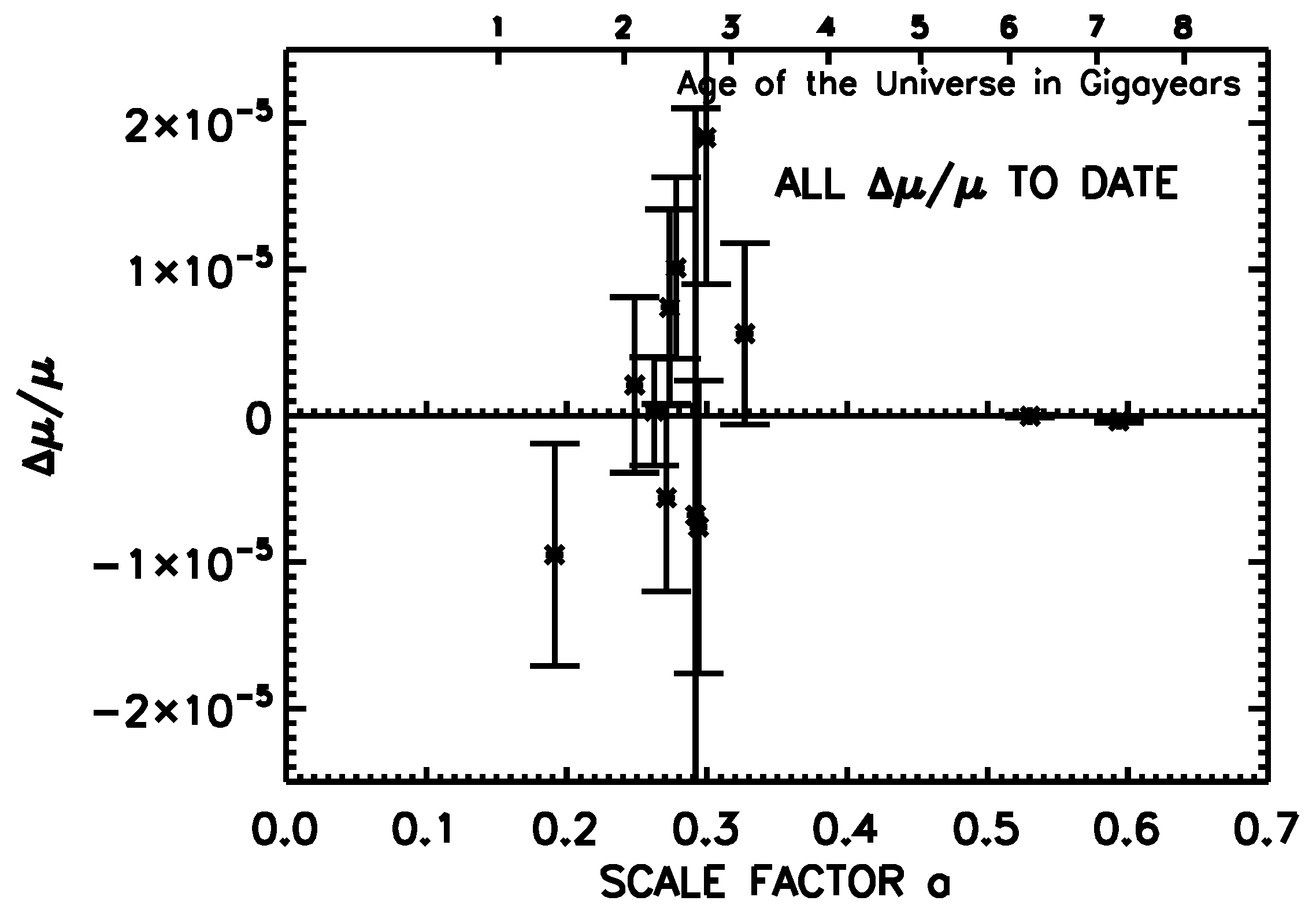
Figure 2.
The low redshift radio constraints at and plotted versus the scale factor . The error bar at is , however, the error bar at () includes systematic effects that increase the error to . That is the primary constraint utilized in this work.
Figure 2.
The low redshift radio constraints at and plotted versus the scale factor . The error bar at is , however, the error bar at () includes systematic effects that increase the error to . That is the primary constraint utilized in this work.

Figure 3.
The figure indicates the 1σ variation of the limit on as a function of the model parameter R. The dashed line indicates the limit on if the measured values of and are used rather than the limits. The dot is at which is the example value. Note that although it is not apparent at the scale of the figure the limit on at is not zero but rather the small term in (11) that does not depend on R.

© 2017 by the author. Licensee MDPI, Basel, Switzerland. This article is an open access article distributed under the terms and conditions of the Creative Commons Attribution (CC BY) license ( http://creativecommons.org/licenses/by/4.0/).
Share and Cite
MDPI and ACS Style
Thompson, R.I. The Relation between Fundamental Constants and Particle Physics Parameters. Universe 2017, 3, 6. https://doi.org/10.3390/universe3010006
AMA Style
Thompson RI. The Relation between Fundamental Constants and Particle Physics Parameters. Universe. 2017; 3(1):6. https://doi.org/10.3390/universe3010006
Chicago/Turabian StyleThompson, Rodger I. 2017. "The Relation between Fundamental Constants and Particle Physics Parameters" Universe 3, no. 1: 6. https://doi.org/10.3390/universe3010006
Note that from the first issue of 2016, this journal uses article numbers instead of page numbers. See further details here.