
Quantum Cosmology and Varying Physical Constants

Institute of Physics, University of Szczecin, Wielkopolska 15, 70-451 Szczecin, Poland
Universe 2017, 3(2), 46; https://doi.org/10.3390/universe3020046
Submission received: 2 April 2017
/
Revised: 14 May 2017
/
Accepted: 15 May 2017
/
Published: 23 May 2017
(This article belongs to the Special Issue Varying Constants and Fundamental Cosmology)
Abstract
:The main task of this review is to discuss quantum cosmology minisuperspace models based on the Wheeler–DeWitt equation, which apart from the standard matter and 3-geometry configuration degrees of freedom, allow those related to the variability of physical constants—varying speed of light (VSL) c and varying gravitational constant G. The tunneling probability of the universe “from nothing” to the Friedmann phase will be given for such varying constants minisuperspace models.
1. Introduction
Some physicists often express their doubts about the statement that constants—which are considered to be fundamental in physics—may vary. However, if we consider them as fields which are influenced by some unknown physical interaction (e.g., of a certain given mass with the rest of the masses in the universe—something which is the core of Brans–Dicke theory, or the influence of extra dimensions), then this statement is just a consequence. Even worse, the Universe as a quantum object may be found to be inherently incompatible as well. After all, cosmology studies the large-scale structure of the Universe, while quantum mechanics seem to be applied to extremely small objects. Here in the same way we may say that since quantum theory is the underlying theory of physics, we should use it to describe the whole universe, possibly deriving our macroscopically classical universe in some limit or due to some mechanism (e.g., decoherence). Besides, the universe surely started with a small size and dense state—the Big-Bang. We could then look for the first epochs of the evolution of the Universe, near the Planck scale of GeV, at which quantum effects cannot be described classically. Another problem which arises when we go back in time to the moment of the birth of the Universe is the initial singularity—a state for which our gravity theory fails. The singularity is considered to be unavoidable on the classical level, through. A way out of this problem may be provided by quantum cosmology, where the birth of the Universe can be described as a quantum phenomenon. The most orthodox Copenhagen interpretation of quantum mechanics considers treating the Universe as a quantum system as problematic; it requires the presence of a classical observer external to the system under consideration. Since it is very difficult to define something external to the Universe, the quantum description may happen to be inadequate in this narrow interpretation. However, one is able to define some internal degrees of freedom which can “measure” the system. The scheme is known as decoherence.
The variability of fundamental constants has been widely investigated in theoretical and experimental physics [1,2,3,4,5,6]. The gravitational constant G, the speed of light c, the electron charge e, the proton-to-electron mass ratio , and the fine structure constant can all be considered as varying [7]. The theories with varying speed of light can provide a solution to some well-known cosmological problems, such as the flatness problem, the horizon problem, the -problem, and the singularity problem [8]. However, most of the studies on varying constants theories were devoted to describe the classical models, and so I want to discuss the quantum aspects of this.
In reference [9], one can find the first attempt to construct the varying constant quantum cosmology with varying c and G, and additionally varying the cosmological constant. The authors calculated the probability of tunneling from “nothing” (i.e., quantum vacuum which depended on varying constants) to the expanding de Sitter space. In reference [10], the probability of the creation of the Universe was calculated for a range of different values of c. The conclusion was that the largest probability of the creation is for the current value of . The results were obtained based on the assumption that the speed of light was decreasing, which was compatible with observations. However, according to the current data [11,12], one should consider both possibilities—a decreasing as well as an increasing value of c.
2. Tunneling Quantum Cosmology
2.1. The Tunneling Universe
As was mentioned already, within the framework of quantum cosmology, one hopes to avoid the problem of the classical initial singularity. It can be achieved in a scenario originally proposed by A. Vilenkin [13,14], in which the Universe is spontaneously created from “nothing” to some specific geometry with a fixed value of the scale factor (the so-called tunneling boundary condition wave function). By “nothing”, it is meant the state where no classical space and time exist, though there is a quantum vacuum.
The evolution equation of the Universe described by a closed Friedmann–Lemaitre–Robertson–Walker universe is solved by the scale factor a:
where
is the Hubble parameter and describes the de Sitter space and is the vacuum energy density. It is very interesting to notice a good analogy to a particle bouncing off the potential barrier at . In this case, a can be treated as a particle coordinate. In quantum mechanics, the probability of tunneling through the finite potential barrier is not zero. Analogously, one assumes that the whole Universe can tunnel through a potential barrier from the vacuum state to a state with a finite value of the scale factor given by . By mapping the problem from Minkowski to Euclidean space (), one can find a solution which describes a four-sphere called the de Sitter instanton:
The above solution describes the tunneling from the de Sitter instanton with an imaginary time to the de Sitter space.
2.2. The Wave Function of the Universe
In analogy to the Schrödinger equation in quantum mechanics, the main equation in quantum cosmology is the Wheeler–DeWitt equation [15,16].
Here is the Hamiltonian operator, is the wave function of the Universe, which is defined on a superspace manifold of all possible 3-geometries and matter-field configurations . It is remarkable that does not depend on a classical cosmological time. However, the lack of a classical time does not mean that the Universe is static—it has its internal clock due to a hyperbolic nature of the Wheeler–DeWitt Equation (4), which makes the scale factor to be a new time coordinate in minisuperspace (a symmetric version of superspace).
In order to solve the Wheeler–DeWitt equation, one needs to specify the appropriate boundary conditions for the wave function. In quantum cosmology, such boundary conditions must be defined independently as a new law. The reason is that one needs to assume that nothing external limits the Universe. Few such wave functions have been proposed so far. One of them is due to A. Vilenkin, and it is called the tunneling wave function [13,14,17,18]. According to this proposal, only the outgoing modes of the wave function should be included on the singular boundaries of the superspace. This means that among all the universes which are described by the function , only the universes which tunnel from nothing to the phase of expansion should be considered. Those which contract down from the infinite size are not taken into account. The tunneling proposal can also be formulated in terms of the path integral over all the paths which interpolate between a vanishing three-geometry ∅ and a state :
These two formulations of the tunneling conditions—the carrying flux out of the superspace and the path integral formulation—are equivalent only in the simplest case of the de Sitter space, not in general.
Another boundary condition assumes that no boundary is the only boundary of the universe. The proposal is called the no-boundary condition, and it was formulated by J. Hartle and S. Hawking in 1983 [19]. The condition is expressed as an Euclidean path integral over compact 4-manifolds bounded by 3-geometry :
where is the Euclidean Einstein–Hilbert action. The no-boundary condition is implemented in the Euclidean regime of the wave function, while the tunneling condition is applied to the Lorentzian (oscillatory) regime. The crucial difference between these two wave functions appears when investigating the prediction for inflation. The function seems to prefer large values of the scalar field , while the function prefers small . Consequently, seems to predict inflation, while predicts no inflation (cf. [20], pp. 279–289).
3. Classical Varying Constants Cosmology
The field equations for the Friedmann universes with varying speed of light and varying gravitational constant varied in a preferred frame read as [6,21,22,23]
The generalized energy-momentum conservation equation is
In the above equations, dots stand for derivatives with respect to the cosmic time t. The scale factor is then denoted by , the pressure by p, the mass density by , , and ±1 is the curvature index. After substituting the vacuum mass density and pressure
into the Equations (7) and (8), one can write down the continuity equation including the -term:
Here, is considered to be a constant. Equation (11) can be written in the form:
After integration, one can obtain the exact solution
where C is a constant and w is a barotropic index from the equation of state . The parameters n and q indicate the possible variation of the constants. In order to describe the dynamics of the change in c and G, the following ansätze has been used [21,24]
The current values of the speed of light and the gravitational constant can be obtained in the limits . These limits are denoted by and , respectively. Different unit ansätze are also possible; i.e.,
4. Quantum Cosmology of Varying Constants
Once the classical equations for varying c and G have been formulated, one can proceed with the quantization. In this work, the canonical quantization will be applied [15,16]. In order to formulate the Wheeler–DeWitt equation, one first needs to find the total action. The gravitational part—the Einstein–Hilbert action—takes the form
where and . The comma stands for the derivative with respect to the new time coordinate . The Friedmann metric can be written as
where , , , , and
In order to obtain a well-defined variational principle, one needs to add to (17) the Gibbons–Hawking–York boundary term
where h is the determinant of the 3-metric defined on the boundary, and K is the trace of the second fundamental form . The matter action is defined as
where is the matter density and is the volume factor, which for is finite
while for can be made finite after an appropriate cut–off [20]. For the cosmological constant , one can write:
The total action is
with L being the Lagrangian. We calculate conjugate momentum as
and the Hamiltonian reads as
Replacing conjugate momentum by an operator
one gets the Wheeler–DeWitt (WDW) equation
with the minisuperspace potential
After quantization of Equation (26), which leads to a stationary Schrödinger Equation (28), one needs to introduce an internal definition of time. This can be done by a new time parametrization in terms of the scale factor a or possibly the matter field . Due to the requirement of self-adjointness of the WDW operator , either choice leads to a different physical Hilbert space. The above-mentioned freedom of the time parametrization is known as the “problem of time” in quantum cosmology. In order to ensure that is Hermitian, some specific boundary conditions for the wave function should be implemented, and this secures the conservation of probability at infinity. Constructing the Hilbert space is a long-standing problem in cosmology, which is beyond the scope of this paper. The problem has already been reviewed in a couple of papers [25,26].
In view of the lack of a classical time in minisuperspace, c and G have been replaced by the scale factor dependence [15]. The ansätze (14) and (15) are valid for a–dependence only, so that we have
For , the minisuperspace potential depends on the matter only due to a dissipative term on the r.h.s. of (11), and reads
The potential (33) has roots at and at
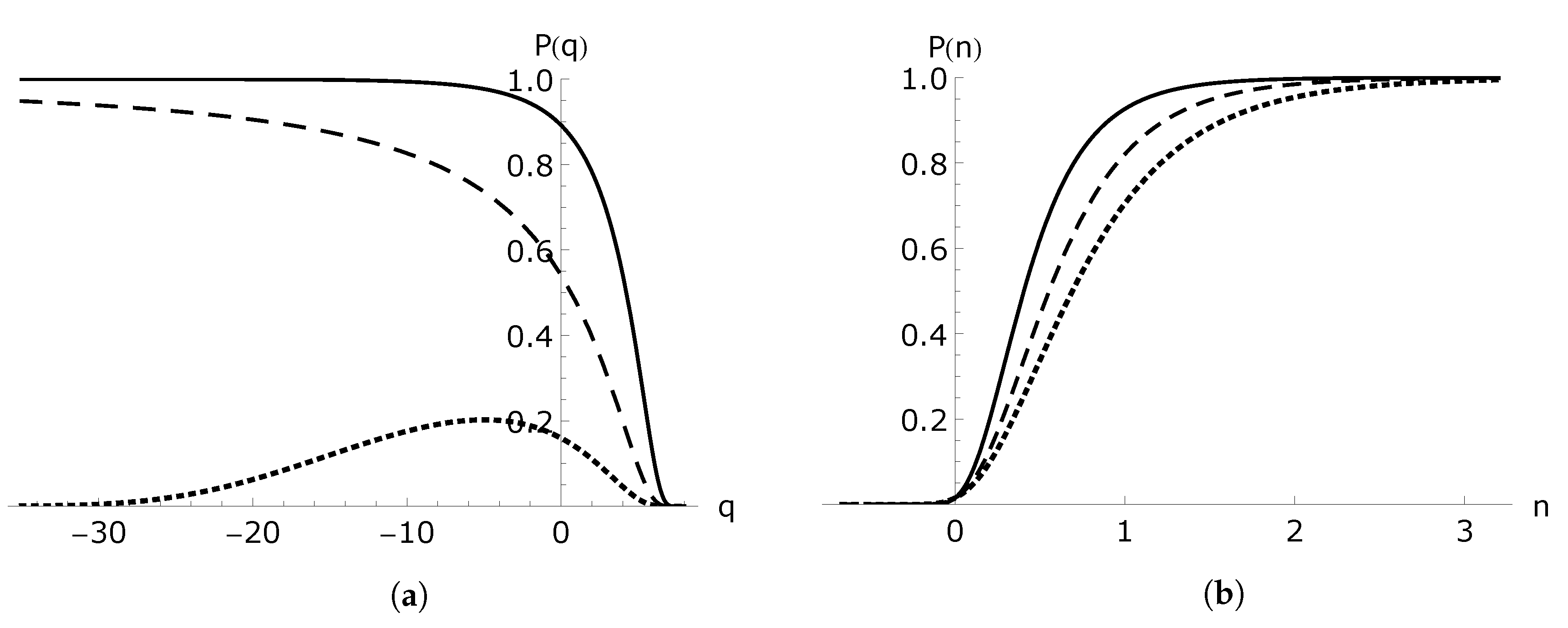
The varying c and G minisuperspace potentials allow the tunneling wave functions, so one can use the WKB approximation to calculate the probability of tunneling from “nothing” to the de–Sitter inflationary Universe with [27]. Having (33), one can write
which is solved by (provided ):
and is the Euler function. Example plots of the tunneling probability are given in Figure 1.
5. Conclusions
In the present paper, the quantum cosmology of varying constants c and G has been discussed. The canonical quantization procedure has been followed. The variability of the speed of light and the gravitational constant have been included by using the ansätze (14) and (15). It has been shown that most of the potentials of varying constants minisuperspace are of the shape which allows the tunneling process. For this reason, the use of WKB approximation is allowed. The probabilities of the tunneling from “nothing” to the Friedmann universe has been calculated. The radius of the newborn universe is characterized by the value of the scale factor . The tunneling interpretation of the creation of the universe allows us to avoid the classical problem of the initial singularity.
It has been shown that the probability of such tunneling depends on the matter content and on the parameters related to the varying constants n and q. The probability increases strongly for positive values of parameter n, while it decreases for negative values of this parameter for all types of matter which have been investigated. The claim of [10] of the greatest probability for the current value of the speed of light () has been shown to be inadequate in the view of current observations of the variability of the fine structure constant . The probability steeply approaches one for the large increase of c. There is also a strong influence of varying G on the probability reported.
Acknowledgments
I thank M.P. Dąbrowski for helpful discussions. This work was supported by the National Science Center Grant DE-2012/06/A/ST2/00395.
Conflicts of Interest
The authors declare no conflict of interest.
References
- Weyl, H. Eine neue Erweiterung der Relativitàtstheorie. Ann. Phys. 1919, 364, 101–133. [Google Scholar] [CrossRef]
- Weyl, H. Universum und Atom. Natturwissenschaften 1934, 22, 145–149. [Google Scholar] [CrossRef]
- Dirac, P.A.M. The Cosmological constants. Nature 1937, 139, 323. [Google Scholar] [CrossRef]
- Dirac, P.A.M. A new basis for cosmology. Proc. R. Soc. A 1938, 165, 199–208. [Google Scholar] [CrossRef]
- Uzan, J.-P. The Fundamental constants and their variation: Observational status and theoretical motivations. Rev. Mod. Phys. 2003, 75, 403. [Google Scholar] [CrossRef]
- Uzan, J.-P. Varying Constants, Gravitation and Cosmology. Living Rev. Rel. 2011, 14, 2. [Google Scholar] [CrossRef] [PubMed]
- Barrow, J.D. The Constants of Nature: From Alpha to Omega–The Numbers that Encode the Deepest Secrets of the Universe; Vintage Books: London, UK, 2002. [Google Scholar]
- Dąbrowski, M.P.; Marosek, K. Regularizing cosmological singularities by varying physical constants. J. Cosmol. Astropart. Phys. 2013, 2013, 012. [Google Scholar] [CrossRef]
- Harko, T; Lu, H.Q.; Mak, M.K.; Cheng, K.S. Quantum birth of the universe in the varying speed of light cosmologies. Europhys. Lett. 2000, 49, 814. [Google Scholar] [CrossRef]
- Szydłowski, M.; Krawiec, A. Dynamical system approach to cosmological models with a varying speed of light. Phys. Rev. D 2003, 68, 063511. [Google Scholar] [CrossRef]
- Webb, J.K.; King, J.A.; Murphy, M.T.; Flambaum, F.F.; Carswell, R.F.; Bainbridge, M.B. Indications of a spatial variation of the fine structure constant. Phys. Rev. Lett. 2011, 107, 191101. [Google Scholar] [CrossRef] [PubMed]
- Murphy, M.T.; Locke, C.R.; Light, P.S.; Luiten, A.N.; Lawrence, J.S. Laser frequency comb techniques for precise astronomical spectroscopy. Mon. Not. R. Astron. Soc. 2012, 422, 761–771. [Google Scholar] [CrossRef]
- Vilenkin, A. Creation of Universes from nothing. Phys. Lett. B 1982, 117, 25–28. [Google Scholar] [CrossRef]
- Vilenkin, A. Birth of inflationary universes. Phys. Rev. D 1983, 27, 2848. [Google Scholar] [CrossRef]
- DeWitt, B.S. Quantum Theory of Gravity. I. The Canonical Theory. Phys. Rev. 1967, 160, 1113. [Google Scholar] [CrossRef]
- Wheeler, J.A. Superspace and the nature of quantum geometrodynamics. In Quantum Cosmology; World Scientific: Singapore, 1987. [Google Scholar]
- Vilenkin, A. Quantum Cosmology and the Initial State of the Universe. Phys. Rev. D 1988, 37, 888. [Google Scholar] [CrossRef]
- Vilenkin, A. Boundary Conditions in Quantum Cosmology. Phys. Rev. D 1986, 33, 3560. [Google Scholar] [CrossRef]
- Hartle, J.B.; Hawking, S.W. Wave function of the Universe. Phys. Rev. D 1983, 28, 2690. [Google Scholar] [CrossRef]
- Kiefer, C. Quantum Gravity—A Short Overview. In Quantum Gravity; Birkhäuser Basel: Basel, Switzerland, 2007. [Google Scholar]
- Barrow, J.D. Cosmologies with varying light speed. Phys. Rev. D 1999, 59, 043515. [Google Scholar] [CrossRef]
- Albrecht, A.; Magueijo, J. A Time varying speed of light as a solution to cosmological puzzles. Phys. Rev. D 1999, 59, 043516. [Google Scholar] [CrossRef]
- Barrow, J.D.; Magueijo, J. Solving the flatness and quasiflatness problems in Brans-Dicke cosmologies with a varying light speed. Class. Quantum Gravity 1999, 16, 1435. [Google Scholar] [CrossRef]
- Gopakumar, P.; Vijayagovindan, G.V. Solutions to cosmological problems with energy conservation and varying c, G and Λ. Mod. Phys. Lett. A 2001, 16, 957–961. [Google Scholar] [CrossRef]
- Feinberg, J.; Peleg, Y. Self-Adjoint Wheeler-DeWitt Operators, the Problem of Time and the wave Function of the Universe. Phys. Rev. D 1995, 52, 1988–2000. [Google Scholar] [CrossRef]
- Carreau, M.; Farhi, E. The Functional Integral for Quantum Systems with Hamiltonians Unbounded from Below. Ann. Phys. 1990, 204, 186–207. [Google Scholar] [CrossRef]
- Atkatz, D. Quantum cosmology for pedestrians. Am. J. Phys. 1994, 62, 619–627. [Google Scholar] [CrossRef]
- Leszczyńska, K.; Balcerzak, A.; Dąbrowski, M.P. Varying constants quantum cosmology. J. Cosmol. Astropart. Phys. 2015, 2, 012. [Google Scholar] [CrossRef]

© 2017 by the author. Licensee MDPI, Basel, Switzerland. This article is an open access article distributed under the terms and conditions of the Creative Commons Attribution (CC BY) license (http://creativecommons.org/licenses/by/4.0/).
Share and Cite
MDPI and ACS Style
Leszczyńska, K. Quantum Cosmology and Varying Physical Constants. Universe 2017, 3, 46. https://doi.org/10.3390/universe3020046
AMA Style
Leszczyńska K. Quantum Cosmology and Varying Physical Constants. Universe. 2017; 3(2):46. https://doi.org/10.3390/universe3020046
Chicago/Turabian StyleLeszczyńska, Katarzyna. 2017. "Quantum Cosmology and Varying Physical Constants" Universe 3, no. 2: 46. https://doi.org/10.3390/universe3020046
Note that from the first issue of 2016, this journal uses article numbers instead of page numbers. See further details here.