QCD Equations of State in Hadron–Quark Continuity

Institute of Particle Physics (IOPP) and Key Laboratory of Quark and Lepton Physics (MOE), Central China Normal University, Wuhan 430079, China
Universe 2018, 4(2), 42; https://doi.org/10.3390/universe4020042
Submission received: 3 January 2018
/
Revised: 12 February 2018
/
Accepted: 13 February 2018
/
Published: 19 February 2018
(This article belongs to the Special Issue Compact Stars in the QCD Phase Diagram)
Abstract
:The properties of dense matter in quantum chromodynamics (QCD) are delineated through equations of state constrained by the neutron star observations. The two solar mass constraint, the radius constraint of ≃11–13 km, and the causality constraint on the speed of sound, are used to develop the picture of hadron–quark continuity in which hadronic matter continuously transforms into quark matter. A unified equation of state at zero temperature and -equilibrium is constructed by a phenomenological interpolation between nuclear and quark matter equations of state.
1. Introduction
The study of the phase structure in quantum chromodynamics (QCD) at large baryon density has been a difficult problem, partly because the lattice Monte Carlo simulations based on the QCD action are not at work, and partly because many-body problems with strong interactions are very complex in theoretical treatments. Currently, the best source of information for dense QCD is the physics of neutron stars from which one can extract useful insights into QCD equations of state [1], as well as the transport properties in matter. Since the domain relevant for these physics is the baryon density of (: nuclear saturation density) or baryon chemical potential of GeV, we can use the neutron star constraints to explore the properties of matter beyond the nuclear regime.
There have been remarkable progress in observations that constrain our understanding on the nature of dense QCD matter. They include the discoveries of two-solar mass () neutron stars [2,3], the constraints for the neutron star radii from X-ray analyses [4,5], and, most remarkably, the detection of the gravitational waves (GW170817) [6] and the electromagnetic signals [7] from the neutron star merger found on 17 August. While the GW170817 was announced only after this meeting, we include this topic in this article because of its significance.
Of particular concern in this article are the constraints on equations of state through the neutron star mass–radius (M-R) relations. In principle, a precisely determined M-R relation can be used to directly reconstruct the neutron star equations of state [8], even without any knowledge about microscopic properties of the matter. Actually, the current precision of M-R relations is not good enough to pin down the unique equation of state. Nevertheless, the current constraints are already significant for us to derive qualitative and semi-quantitative understanding about the nature of dense QCD matter.
Based on equations of state supposed from the M-R and causality constraints, we will develop the picture of hadron–quark continuity in which hadronic matter continuously transforms into quark matter without experiencing thermodynamic phase transitions. Such continuity picture was developed in the context of the crossover from the superfluid hadronic phase to the color-flavor-locked superconducting phase [9]. This scenario was revisited in [10,11] where the role of anomaly is emphasized. The previous studies are based on theoretical considerations and model calculations, while, in our approach, we reach the continuity picture from the demand to satisfy the neutron star constraints.
2. The Neutron Star Constraints and the Implications for QCD Equations of State
To begin with, we first define some terminology in this article. “Stiff” equations of state mean equations of state with large pressure P at given energy density . The stiffer equations of state generally lead to larger maximum masses and larger radii for neutron stars. We will not use the speed of sound as the measure of the stiffness, as even ideal gas equations of state with the relatively small sound velocity (compared to what we will consider) can generate very large maximum masses.
Secondly, we should specify at which region of density the equations of state are stiff. We will use the terminology such as “soft-stiff”, by which we mean that equations of state is soft at low density, , and stiff at high density, . For the reasons described below, equations of state leading to km for stars will be called “soft at low density”, and equations of state leading to will be called “stiff at high density’. Then, the soft-stiff equations of state generate the M-R curves with the typical radii of km and the maximum mass ≥2.
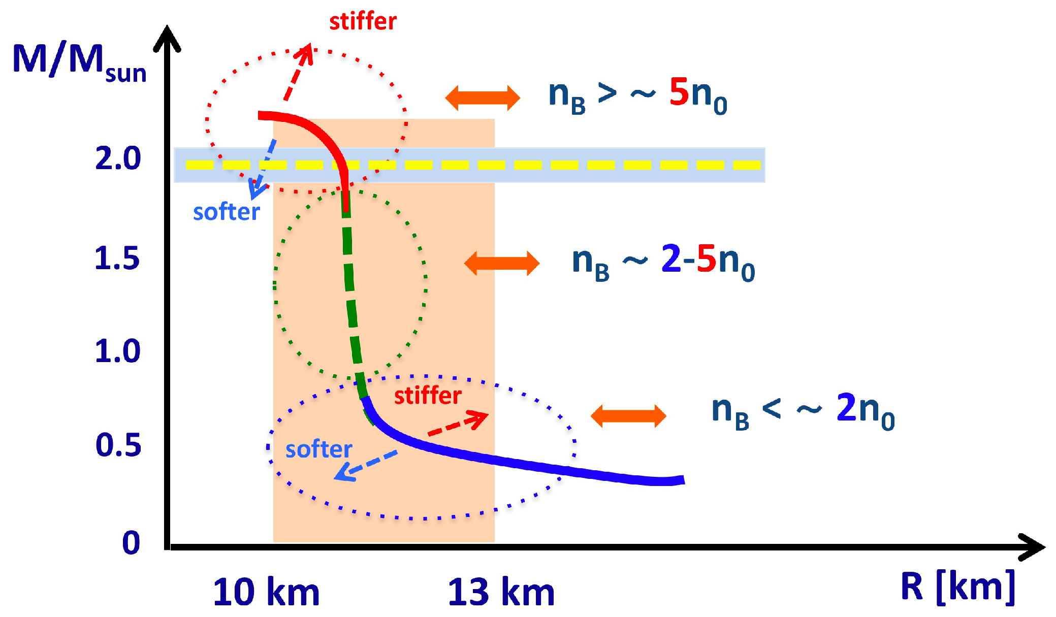
The classification of equations of state by the baryon density is useful because it has been known [12] that the shapes of the M-R curves have strong correlations with equations of state at several fiducial densities (see Figure 1). At very low density, the material is loosely bound by the gravity, but, as M increases, R rapidly decreases because of the stronger gravity. Around ∼2, the matter starts to observe the repulsive forces in microscopic dynamics; then, the M-R curve starts to go vertically. Eventually, the curve reaches the maximum in M at . Using these correlations between M-R and , one can focus on the radius constraint in the studies of low density equations of state, or one can focus on the maximum mass when studying high density equations of state.
The existence of two-solar mass () neutron stars [2,3] tells us that high density equations of state at must be stiff. Meanwhile the estimate of is relatively uncertain. There have been many theoretical predictions for which range from ≃10 km to ≃16 km. The observational constraints on , which have been based on spectroscopic analyses of the X-rays from the neutron star surface, include several systematic uncertainties, but the current trend converges toward the estimate R = 11–13 km 1. In addition, the analyses of gravitational waves from GW170817 favors equations of state with the radii smaller than ∼13 km. More precisely, the actual constraint is on the dimensionless tidal deformability, (: Newton constant; : Love number [16]), of each star before the coalescence; clearly is very sensitive to the compactness and radius of the star.
Therefore, the QCD equation of state is likely to be the soft-stiff type. For the left over region , there is also a causality constraint on the speed of sound , i.e., must be less than the light velocity 2. This constraint becomes significant for soft-stiff equations of state because is small at low density but must be large at high density, meaning that in between there must be a region where must be large. The difficulty is even more signified if there are the first order phase transitions, see Figure 2; during such transitions, is constant for increasing , and, after the phase transitions, even larger is necessary to get connected to at high density.
If we assume the neutron star radii to be large km, then the equations of state at low density is so stiff that, even after strong 1st order phase transitions, the low density equations of state have the causal connection to at high density [17]. Thus, the determination of the neutron star radii is crucial for our understanding of the QCD phase structure. It should be evident that if the strength of transitions is sufficiently weak, the soft-stiff equations of state is still possible even with the 1st order transitions. For more quantitative and systematic analyses, we refer to Ref. [18].
These considerations for soft-stiff equations of state motivate us to consider the picture of hadron–quark continuity in which equations of state at and are continuously connected.
3. The 3-Window Modeling
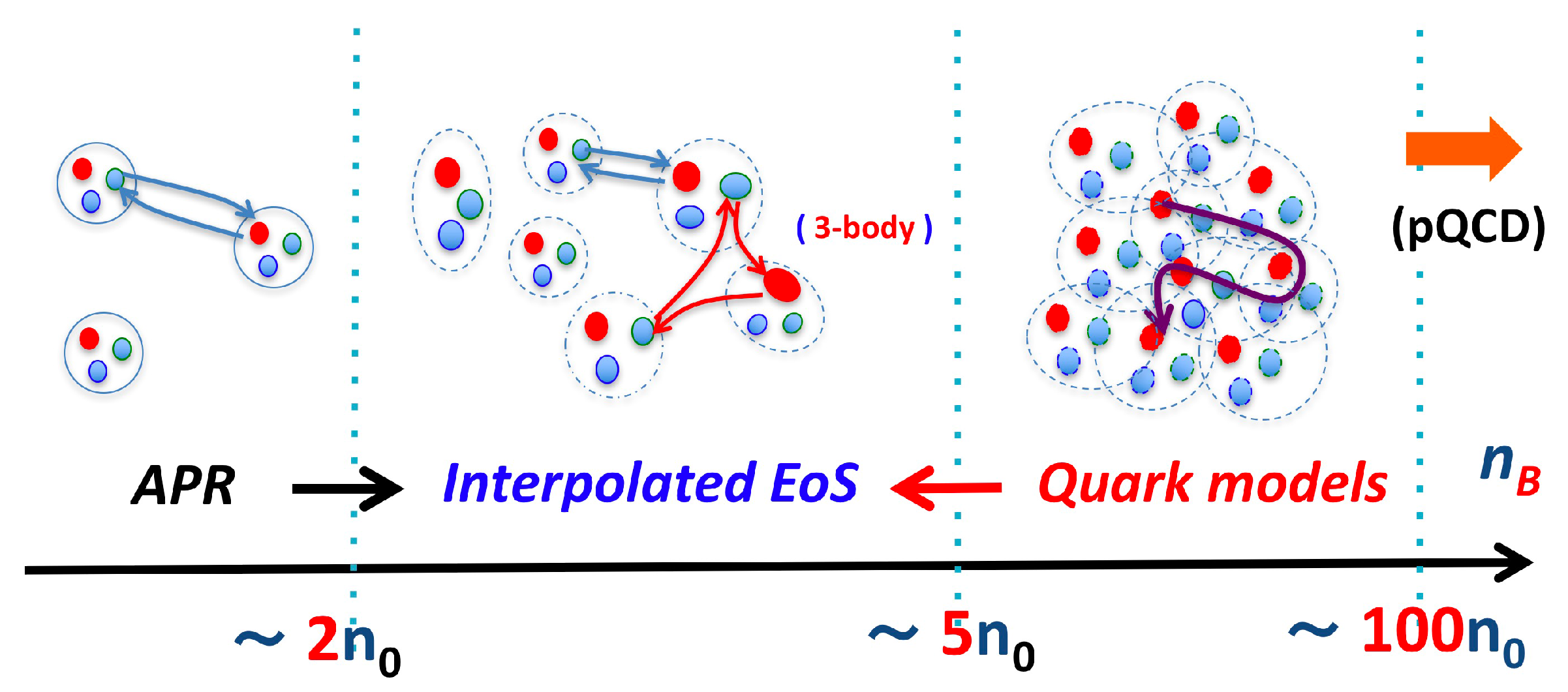
Now, we turn to the discussions about the microscopic nature of matter. We consider the matter by decomposing it into 3-windows [19,20,21,22]; the nuclear regime at ; the crossover regime for ; and the quark matter regime at . The picture we have is illustrated in Figure 3. At low density, , the matter is dilute and baryons remain well-defined objects, so the equations of state are described by nuclear ones. Beyond ∼, it is unlikely that nucleons are effective degrees of freedom; many-body forces become increasingly important as seen from microscopic nuclear calculations, which include nuclear interaction up to 3-body forces [23,24], and, in addition, typical calculations indicate that baryonic excitations other than nucleons are no longer negligible. Even though the matter is presumably not dense enough to consider quark matter, the above-mentioned problems demand us to think of matter based on microscopic quark degrees of freedom. At ∼, baryons with the radii of ∼0.5 fm start to touch one another. If we assume a 3-flavor quark matter, the density corresponds to the quark Fermi momentum of ∼400 MeV (for 2-flavor matter is even larger), reasonably large compared to the QCD non-perturbative scale, 200.
One might think that, since some phenomenological hadronic equations of state have been made consistent with the constraint (e.g., [23]), there is no need to introduce the quark matter descriptions for neutron star matter. However, to pass the constraint is the necessary but not sufficient condition to validate the hadronic models; the construction of equations of state must be reasonable from the microscopic point of view, but, at this point, we have problems in extrapolating purely hadronic descriptions beyond , for the reasons already discussed above. This motivates us to start with quark matter picture at high density side and approach the hadronic side by including hadronic correlations. This approach, even when ∼ happens to not be high for the quark matter formation, at least will shed light on the nature of hadronic matter in terms of quark descriptions.
We will construct equations of state based on this 3-window picture. For the nuclear regime, we use the Akmar–Phandheripande–Ravenhall (APR) equation of state as a representative 3 [23]. For the quark matter regime, we use a schematic quark model that concisely expresses microscopic interactions relevant in hadron and nuclear physics. In between, neither purely hadronic nor quark matter descriptions are appropriate, so here we use the hadron–quark continuity picture to smoothly interpolate the APR and quark model equations of state. Specifically, our interpolation is done with polynomials [21]
To determine the coefficients s, we first compute , and then demand, at and , the interpolating function to match with the APR and quark equations of state up to the second order derivatives of .
4. A Model for Quark Matter
In our phenomenological modeling, we need to choose a quark model for . Guided by the continuity picture, the form of effective models is exported from those for hadron physics. Here, semi-long range interactions, relevant for the energy scale of 0.2–1 or distance scale ∼0.2–1 [25], should remain important from low to high densities because the quark matter regime observes the contents inside of hadrons. Meanwhile, due to the overlap of baryon wavefunctions, the confining forces that try to neutralize the color are expected to be less important at higher densities, except for any excitations that break the local color neutrality. The confining force is a long range interaction relevant for the energy scale 0.2∼1 .
Our effective Hamiltonian is () [1]
The first line is the standard Nambu-Jona-Lasinio (NJL) model with -quarks and responsible for the chiral symmetry breaking. We use the Hatsuda–Kunihiro parameter set [26] with which the constitutent quark masses are and . The first term in the second line includes the confining interactions which trap 3-quarks into a baryon. The second term is the color-magnetic interaction for color-flavor-antisymmetric S-wave channel; they play very important roles in the level splitting in the hadron spectra, e.g., N- splitting. The last term is the phenomenological vector repulsive interactions, which are inspired from the -meson exchange in nuclear physics. In actual calculations, the confining term is not explicitly included as we do not know a good modeling for it. Therefore, we restrict the use of this model to where we expect that confining effects are not significant.
While the form of the Hamiltonian is obtained by extrapolating the description of hadron and nuclear physics, in principle the range of parameters at can be considerably different from those used in hadron physics due to, e.g., medium screening effects. In a strongly correlated region, the estimate of medium modifications is difficult; for instance, screening masses in 2-color QCD, measured in lattice QCD [27], are qualitatively different from the perturbative behaviors [28]. For 3-color QCD, no reliable estimates on medium modifications are available, so here we use the neutron star constraints to examine the range of these parameters, and then use them to delineate the properties of QCD matter at . Below, we vary (, while assuming that do not change from the vacuum values appreciably; this assumption will be checked posteriori. More elaborated treatment is to explicitly determine the medium running coupling , as demonstrated in Ref. [29].
Our Hamiltonian for quarks, together with the contributions from leptons, is solved within the mean field (MF) approximation. We impose the neutrality conditions for electric and color charges as well as the -equilibrium condition. In the MF treatments, we find that the chiral and diquark condensates coexist at . For the range of parameters that we have explored, the diquark pairing always appears to be the color-flavor-locked (CFL) type at ; other less symmetric pairings such as the 2SC type appear only at lower density, thus we will not take their appearance at face value.
Now, we examine the roles of effective interactions by subsequently adding and then H to the standard NJL model [21]. First of all, in order to make equations of state stiff, should remain comparable to the size of its vacuum values; the large reduction of these parameters accelerates the chiral restoration that yields contributions similar to the bag constant, i.e., the positive (negative) contributions to energy (pressure). As a result, the significant softening takes place in equations of state. Actually, even if we fix to the vacuum values, the strong 1st order chiral transition takes place at ∼2–3 in the standard NJL model, so the equations of state at is too soft to pass the constraint.
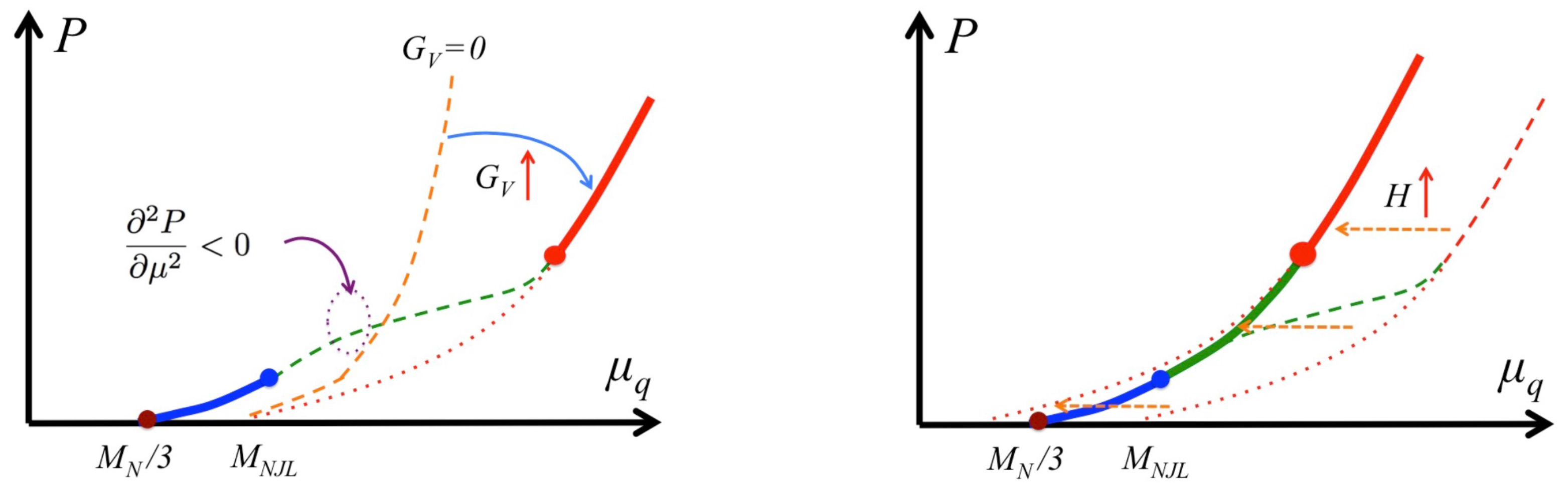
This situation is changed by adding . It stiffens the equations of state in two-fold ways. Firstly, the repulsive interactions obviously contribute to the stiffening. Secondly, it delays the chiral restoration by tempering the growth of baryon density as a function of , so that there is no radical softening associated with the chiral restoration. In fact, the 1st order transition turns into a crossover in the range of we explored. The value of large enough to pass the constraint, however, causes another kind of problem in connecting the APR and quark model pressure; see the left panel of Figure 4; with larger quark pressure, tends to appear at higher with less slope, and, as a consequence, the pressure curve in the interpolation region tends to contain an inflection point at which is negative. Such region is thermodynamically unstable and so must be excluded. Therefore, while a larger value of is favored to pass the constraint, it generates more mismatch between the APR and quark pressure in the direction.
Here, the color-magnetic interactions improve the situation; see the right panel of Figure 4. We note that the onset chemical potential of the APR pressure is the nucleon mass , while, for the NJL pressure, it is . In a conventional picture of quark models, the nucleon and masses are split by the color-magnetic interaction, and the nucleon mass is reduced from . From this viewpoint, the color-magnetic interactions naturally induce the overall shift of the NJL pressure toward the lower chemical potential, thus making the matching between the APR and quark pressure curves much better.
The M-R relations are shown in Figure 5 for the parameter sets , and . For all these sets, the radius of a neutron star at the canonical mass is 11.3–11.5 km, mainly determined by our APR equations of state. In these sets, only the set fulfills all of the constraints; the set is slightly below the constraint, while slightly violates the causality bound. More exhaustive parameter surveys [1] show that should be 0.7 , and 1.4 which are comparable to the vacuum scalar coupling. For given , the value of H is fixed to ∼10%; in fact, we do not have much liberty in our choice when we connect the APR and quark matter pressures.
We note that the couplings as large as the vacuum coupling of are necessary to fulfill the constraints from neutron star observations and causality. With such strong effective couplings, we expect that gluons in the non-perturbative regime still survive in spite of the presence of quark matter. In addition, substantial amounts of chiral and diquark condensates coexist [21]. It is also important to emphasize that the quark matter contains the strange-quarks as much as up- and down-quarks.
5. Discussion and Conclusion
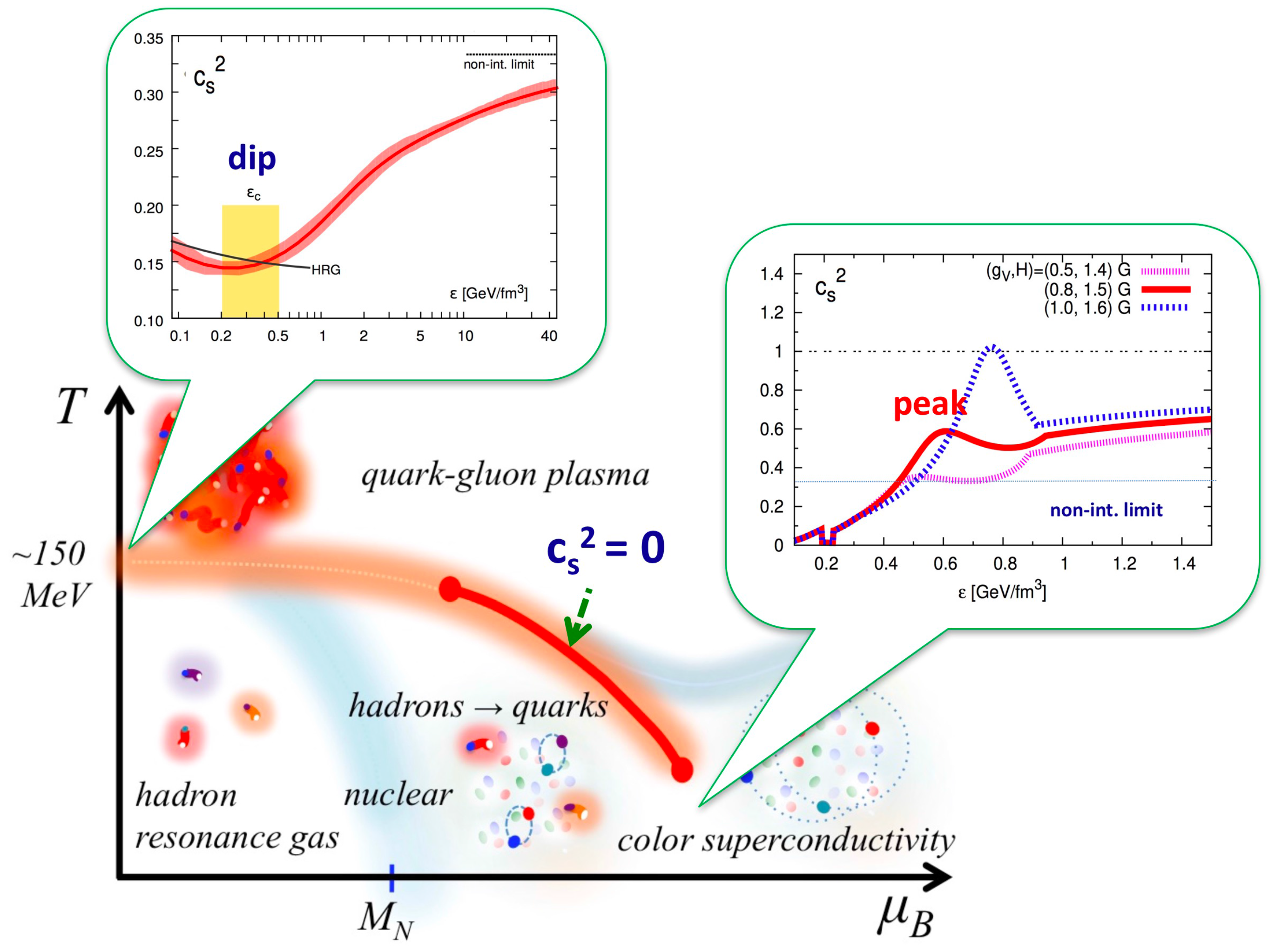
We first mention the difference between the finite temperature crossover and low temperature crossover (see Figure 6). The relevant thermodynamic relations are (s: entropy) and , respectively. In the finite temperature crossover, which has been established by the lattice Monte Carlo calculations [30,31], the QCD matter changes from a hadron resonance gas to a quark gluon plasma as the temperature increases. The transition is smooth, but radical changes take place in the thermodynamic quantities. In particular, there is radical growth in the entropy and energy densities as a consequence of liberation of quarks and gluons, which in turn lead to a dip in the speed of sound . In contrast, this feature is not present in the low temperature crossover; the sound velocity should have a peak, rather than a dip, in the crossover region [1]. Neither the baryon density nor energy density radically change; instead, as the matter approaches the crossover region, the strong interactions among baryons temper the growth of the baryon density at increasing . In this respect, the distinction between strongly interacting hadronic and quark matter is more difficult than that between a hadron resonance gas and a quark gluon plasma. It may be appropriate to characterize the hadron–quark crossover in terms of the quark–hadron duality, or in the context of quarkyonic matter [32,33,34,35] that has the quark Fermi sea but baryonic Fermi surface; hence, it naturally interpolates the hadronic and quark matter. To get qualitative insights for the quarkyonic matter, we refer to the studies of QCD in (1+1) dimensions [36] where analytic insights are available.
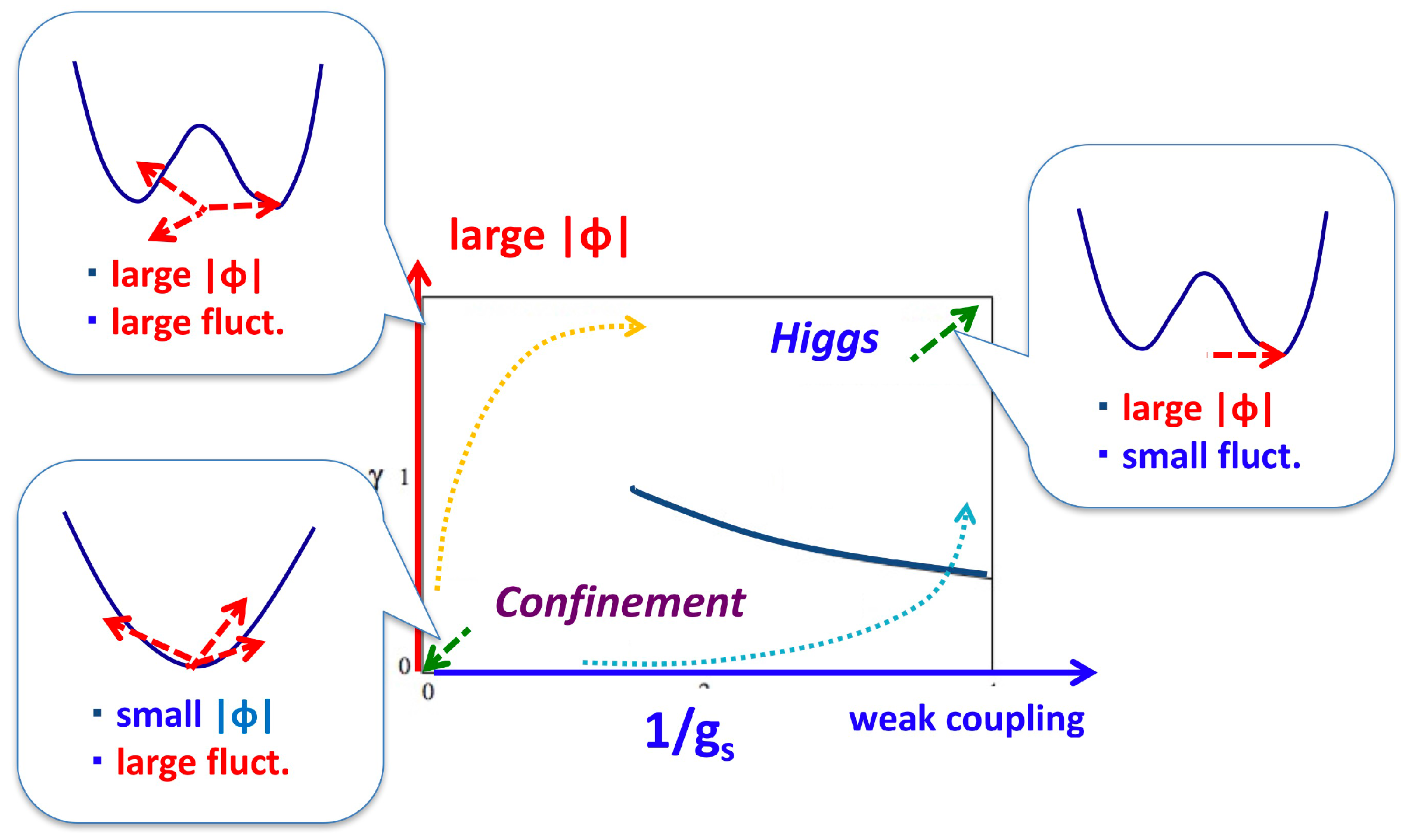
Finally, we present a conjecture concerning the crossover in the gauge dynamics, namely from a confining phase to a Higgs phase with colored diquark condensates ∼. This question must be addressed when we consider the crossover from hadronic to quark matter with diquark condensates. In the presence of matter fields in the fundamental representations, there are no strict order parameters based on symmetries, and in fact the two phases can be smoothly connected [37]. On the other hand, the symmetry concepts are not necessary conditions for phase transitions, as can be seen in liquid–gas phase transition. Thus, we need to discuss the dynamical aspects. As for the confining vs. Higgs phases, there are two important elements to distinguish them in qualitative terms. The first is the strength of the gauge coupling, , and the other is the size of Higgs field (diquark) amplitudes, . Two extreme limits are relatively easy to imagine: in the strong coupling limit and small Higgs amplitudes, the strong color fluctuations disfavor the colored objects and the confinement takes place [38]. Meanwhile, in the weak coupling limit and large Higgs amplitudes, the matter should look like a Higgs phase as in textbook examples. The important question is how they can be connected depending on the trajectories of the and as functions of .
This question is hard to answer for dense QCD, but some insights can be obtained from the gauge Higgs models with the fixed Higgs amplitude [37]. There are two characteristic paths from the confining to the Higgs phase (see Figure 7). In the first path, we move along the small region in the confining phase; move from to domain, and then go to the domain of . In this path, we hit the phase transition increasing the value of at the weak coupling region. Indeed, it is difficult to imagine that the Higgs phase at weak coupling, which apparently looks very different from the confining phase, continuously transforms into the confining phase. The other path, however, allows the crossover transition: starting again from , , one can move along the region with increasing , and reaches the confining phase at large Higgs fields, or Higgs phase at strong coupling. This regime was not studied as much as the weak coupling regime in quark matter.
From this example and neutron star constraints, we conjecture that the matter remains strongly coupled from hadronic to quark matter regimes, so that the Higgs fields develop within the confining regime and then the system gradually relaxes to the Higgs phase at weak coupling. Gluons remain non-perturbative until the weak coupling regime is reached at sufficiently high density.
More observational constraints will come in the next 10 years through the timing analyses of X-rays in the NICER program [39] and the GW detection by currently operating aLIGO, Virgo, GEO [40], and also KAGRA [41] under construction, which will be ready soon. The electromagnetic counterparts associated with the GWs give the information about the ejecta, from which one can learn the dynamics at the coalescence regime. It is desirable to utilize all this information to improve our understanding of dense QCD matter.
Acknowledgments
The author thanks Gordon Baym, Kenji Fukushima, Tetsuo Hatsuda, Phillip Powell, Yifan Song, Tatsuyuki Takatsuka for collaboration, and D. Blaschke for information about references for neutron star radii. T.K. is grateful for the workshop organizers and participants who made this workshop very enjoyable. This work is supported by an NSFC grant 11650110435.
Conflicts of Interest
The author declares no conflicts of interest.
References
- Baym, G.; Hatsuda, T.; Kojo, T.; Powell, P.D.; Song, Y.; Takatsuka, T. From hadrons to quarks in neutron stars: A review. arXiv, 2017; arXiv:1707.04966. [Google Scholar]
- Demorest, P.; Pennucci, T.; Ransom, S.; Roberts, M.; Hessels, J. Shapiro Delay Measurement of A Two Solar Mass Neutron Star. Nature 2010, 467, 1081–1083. [Google Scholar] [CrossRef] [PubMed]
- Antoniadis, J.; Freire, P.C.C.; Wex, N.; Tauris, T.M.; Lynch, R.S.; van Kerkwijk, M.H.; Kramer, M.; Bassa, C.; Dhillon, V.S.; Driebe, T.; et al. A Massive Pulsar in a Compact Relativistic Binary. Science 2013, 340, 1233232. [Google Scholar] [CrossRef] [PubMed]
- Ozel, F.; Freire, P. Masses, Radii, and Equation of State of Neutron Stars. Ann. Rev. Astron. Astrophys. 2016, 54, 401–440. [Google Scholar] [CrossRef]
- Steiner, A.W.; Lattimer, J.M.; Brown, E.F. Neutron Star Radii, Universal Relations, and the Role of Prior Distributions. Eur. Phys. J. A 2016, 52, 18. [Google Scholar] [CrossRef]
- Abbott, B.P.; Abbott, R.; Abbott, T.D.; Acernese, F.; Ackley, K.; Adams, C.; Adams, T.; Addesso, P.; Adhikari, R.X.; Adya, V.B.; et al. GW170817: Observation of Gravitational Waves from a Binary Neutron Star Inspiral. Phys. Rev. Lett. 2017, 119, 161101. [Google Scholar] [PubMed]
- Abbott, B.P.; Abbott, R.; Abbott, T.D.; Acernese, F.; Ackley, K.; Adams, C.; Adams, T.; Addesso, P.; Adhikari, R.X.; Adya, V.B.; et al. Multi-messenger observations of a binary neutron star merger. Astrophys. J. Lett. 2017, 848, L1–L59. [Google Scholar] [CrossRef]
- Lindblom, L. Determining the nuclear equation of state from neutron-star masses and radii. Astrophys. J. 1992, 398, 569–573. [Google Scholar] [CrossRef]
- Schäfer, T.; Wilczek, F. Continuity of quark and hadron matter. Phys. Rev. Lett. 1999, 82, 3956–3959. [Google Scholar] [CrossRef]
- Hatsuda, T.; Tachibana, M.; Yamamoto, N.; Baym, G. New critical point induced by the axial anomaly in dense QCD. Phys. Rev. Lett. 2006, 97, 122001. [Google Scholar] [CrossRef] [PubMed]
- Zhang, Z.; Fukushima, K.; Kunihiro, T. Number of the QCD critical points with neutral color superconductivity. Phys. Rev. D 2009, 79, 014004. [Google Scholar]
- Lattimer, J.M.; Prakash, M. Neutron Star Observations: Prognosis for Equation of State Constraints. Phys. Rep. 2007, 442, 109–265. [Google Scholar] [CrossRef]
- Suleimanov, V.; Poutanen, J.; Revnivtsev, M.; Werner, K. Neutron star stiff equation of state derived from cooling phases of the X-ray burster 4U 1724-307. Astrophys. J. 2011, 742, 122. [Google Scholar] [CrossRef]
- Nättilä, J.; Steiner, A.W.; Kajava, J.J.E.; Suleimanov, V.F.; Poutanen, J. Equation of state constraints for the cold dense matter inside neutron stars using the cooling tail method. Astron. Astrophys. 2016, 591, A25. [Google Scholar] [CrossRef]
- Nättilä, J.; Miller, M.C.; Steiner, A.W.; Kajava, J.J.E.; Suleimanov, V.F.; Poutanen, J. Neutron star mass and radius measurements from atmospheric model fits to X-ray burst cooling tail spectra. Astron. Astrophys. 2017, 608, A31. [Google Scholar] [CrossRef]
- Hinderer, T.; Lackey, B.D.; Lang, R.N.; Read, J.S. Tidal deformability of neutron stars with realistic equations of state and their gravitational wave signatures in binary inspiral. Phys. Rev. D 2010, 81, 123016. [Google Scholar] [CrossRef]
- Benic, S.; Blaschke, D.; Alvarez-Castillo, D.E.; Fischer, T.; Typel, S. A new quark-hadron hybrid equation of state for astrophysics—I. High-mass twin compact stars. Astron. Astrophys. 2015, 577, A40. [Google Scholar] [CrossRef]
- Alford, M.G.; Han, S.; Prakash, M. Generic conditions for stable hybrid stars. Phys. Rev. D 2013, 88, 083013. [Google Scholar] [CrossRef]
- Masuda, K.; Hatsuda, T.; Takatsuka, T. Hadron-Quark Crossover and Massive Hybrid Stars with Strangeness. Astrophys. J. 2013, 764, 12. [Google Scholar] [CrossRef]
- Masuda, K.; Hatsuda, T.; Takatsuka, T. Hadron-quark crossover and massive hybrid stars. Prog. Theor. Exp. Phys. 2013, 2013, 073D01. [Google Scholar] [CrossRef]
- Kojo, T.; Powell, P.D.; Song, Y.; Baym, G. Phenomenological QCD equation of state for massive neutron stars. Phys. Rev. D 2015, 91, 045003. [Google Scholar] [CrossRef]
- Kojo, T. Phenomenological neutron star equations of state: 3-Window modeling of QCD matter. Eur. Phys. J. A 2016, 52, 51. [Google Scholar] [CrossRef]
- Akmal, A.; Pandharipande, V.R.; Ravenhall, D.G. The Equation of state of nucleon matter and neutron star structure. Phys. Rev. C 1998, 58, 1804. [Google Scholar] [CrossRef]
- Togashi, H.; Nakazato, K.; Takehara, Y.; Yamamuro, S.; Suzuki, H.; Takano, M. Nuclear equation of state for core-collapse supernova simulations with realistic nuclear forces. Nucl. Phys. A 2017, 961, 78–105. [Google Scholar] [CrossRef]
- Manohar, A.; Georgi, H. Chiral Quarks and the Nonrelativistic Quark Model. Nucl. Phys. B 1984, 234, 189–212. [Google Scholar] [CrossRef]
- Hatsuda, T.; Kunihiro, T. QCD phenomenology based on a chiral effective Lagrangian. Phys. Rep. 1994, 247, 221–367. [Google Scholar] [CrossRef]
- Hajizadeh, O.; Boz, T.; Maas, A.; Skullerud, J.I. Gluon and ghost correlation functions of 2-color QCD at finite density. arXiv, 2017; arXiv:1710.06013. [Google Scholar]
- Kojo, T.; Baym, G. Color screening in cold quark matter. Phys. Rev. D 2014, 89, 125008. [Google Scholar] [CrossRef]
- Fukushima, K.; Kojo, T. The Quarkyonic Star. Astrophys. J. 2016, 817, 180. [Google Scholar] [CrossRef]
- Aoki, Y.; Endrodi, G.; Fodor, Z.; Katz, S.D.; Szabo, K.K. The Order of the quantum chromodynamics transition predicted by the standard model of particle physics. Nature 2006, 443, 675–678. [Google Scholar] [CrossRef] [PubMed]
- Ding, H.T.; Karsch, F.; Mukherjee, S. Thermodynamics of strong-interaction matter from Lattice QCD. Int. J. Mod. Phys. E 2015, 24, 1530007. [Google Scholar] [CrossRef]
- McLerran, L.; Pisarski, R.D. Phases of cold, dense quarks at large N(c). Nucl. Phys. A 2007, 796, 83. [Google Scholar] [CrossRef]
- Kojo, T.; Hidaka, Y.; McLerran, L.; Pisarski, R.D. Quarkyonic Chiral Spirals. Nucl. Phys. A 2010, 843, 37–58. [Google Scholar] [CrossRef]
- Kojo, T.; Pisarski, R.D.; Tsvelik, A.M. Covering the Fermi Surface with Patches of Quarkyonic Chiral Spirals. Phys. Rev. D 2010, 82, 074015. [Google Scholar] [CrossRef]
- Kojo, T.; Hidaka, Y.; Fukushima, K.; McLerran, L.D.; Pisarski, R.D. Interweaving Chiral Spirals. Nucl. Phys. A 2012, 875, 94–138. [Google Scholar]
- Kojo, T. A (1+1) dimensional example of Quarkyonic matter. Nucl. Phys. A 2012, 877, 70. [Google Scholar] [CrossRef]
- Fradkin, E.H.; Shenker, S.H. Phase Diagrams of Lattice Gauge Theories with Higgs Fields. Phys. Rev. D 1979, 19, 3682–3697. [Google Scholar] [CrossRef]
- Wilson, K.G. Confinement of Quarks. Phys. Rev. D 1974, 10, 2445–2459. [Google Scholar] [CrossRef]
- Gendreau, K.C.; Arzoumanian, Z.; Adkins, P.W.; Albert, C.L.; Anders, J.F.; Aylward, A.T.; Baker, C.L.; Balsamo, E.R.; Bamford, W.A.; Benegalrao, S.S.; et al. The Neutron star Interior Composition Explorer (NICER): Design and development. Proc. SPIE 2016, 9905, 99051H. [Google Scholar]
- Hough, J.; Meers, B.J.; Newton, G.P.; Robertson, N.A.; Ward, H.; Leuchs, G.; Niebauer, T.M.; Rüdiger, A.; Schilling, R.; Schinupp, L.; et al. Proposal for a Joint German-British Interferometric Gravitational Wave Detector. Available online: eprints.gla.ac.uk/114852/7/114852.pdf (accessed on 3 September 2017).
- Aso, Y.; Michimura, Y.; Somiya, K.; Ando, M.; Miyakawa, O.; Sekiguchi, T.; Tatsumi, D.; Yamamoto, H. Interferometer design of the KAGRA gravitational wave detector. Phys. Rev. D 2013, 88, 043007. [Google Scholar]
| 1. | The exception can be found in [13], where the authors (Suleimanov et al.) estimate km using the X-ray burst from 4U 1724-307. The paper was published in 2011. Later, further analyses were done by two of the authors and their collaborators. In a recent paper [14], they discussed that the event used to extract km is not suitable for reliable analyses due to large contaminations in the neutron star atmosphere. The newer analyses include more samples and cleaner events than the previous ones, and yield the estimate 11 km km for neutron stars with the masses ranging from 1.1–2.1 [15]. The author appreciates Dr. David Blaschke for mentioning these papers. |
| 2. | Some people postulated that the should be smaller than the conformal limit (c: light velotiy). As argued by Bedaque and Steiner, this hypothesis is in tension with the neutron star observations. |
| 3. | Actually, we also need to use some crust equations of state for . We use the Togashi equation of state [24], which is based on the microscopic calculations with techniques similar to the APR, and is consistent with the regime of laboratory nuclei below the neutron drip regime. |
Figure 1.
The correlation between the M-R relation and equations of state.

Figure 2.
The pressure vs. energy density for soft-stiff (left) and stiff-stiff (right) equations of state. The slope is given by , the sound speed square, which must be smaller than the light speed, 1. The soft-stiff equations of state have smaller radii than the stiff-stiff ones, and disfavor the strong 1st order phase transitions.
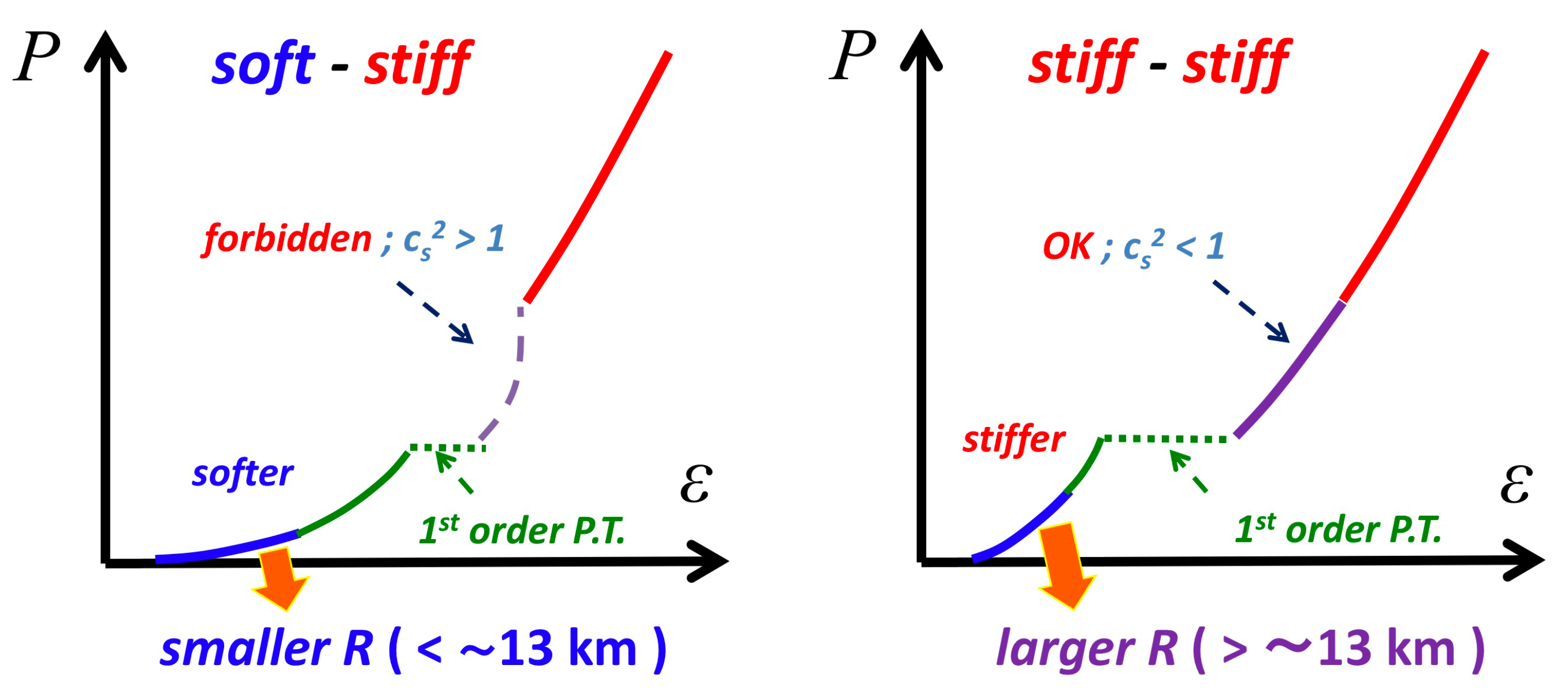
Figure 3.
The 3-window modeling of the QCD matter.

Figure 4.
The impacts of the vector and color-magnetic interactions.

Figure 5.
The mass–radius relations from the 3-window equations of state for sets of parameters, . Only the set satisfies the and causality constraints.
Figure 5.
The mass–radius relations from the 3-window equations of state for sets of parameters, . Only the set satisfies the and causality constraints.
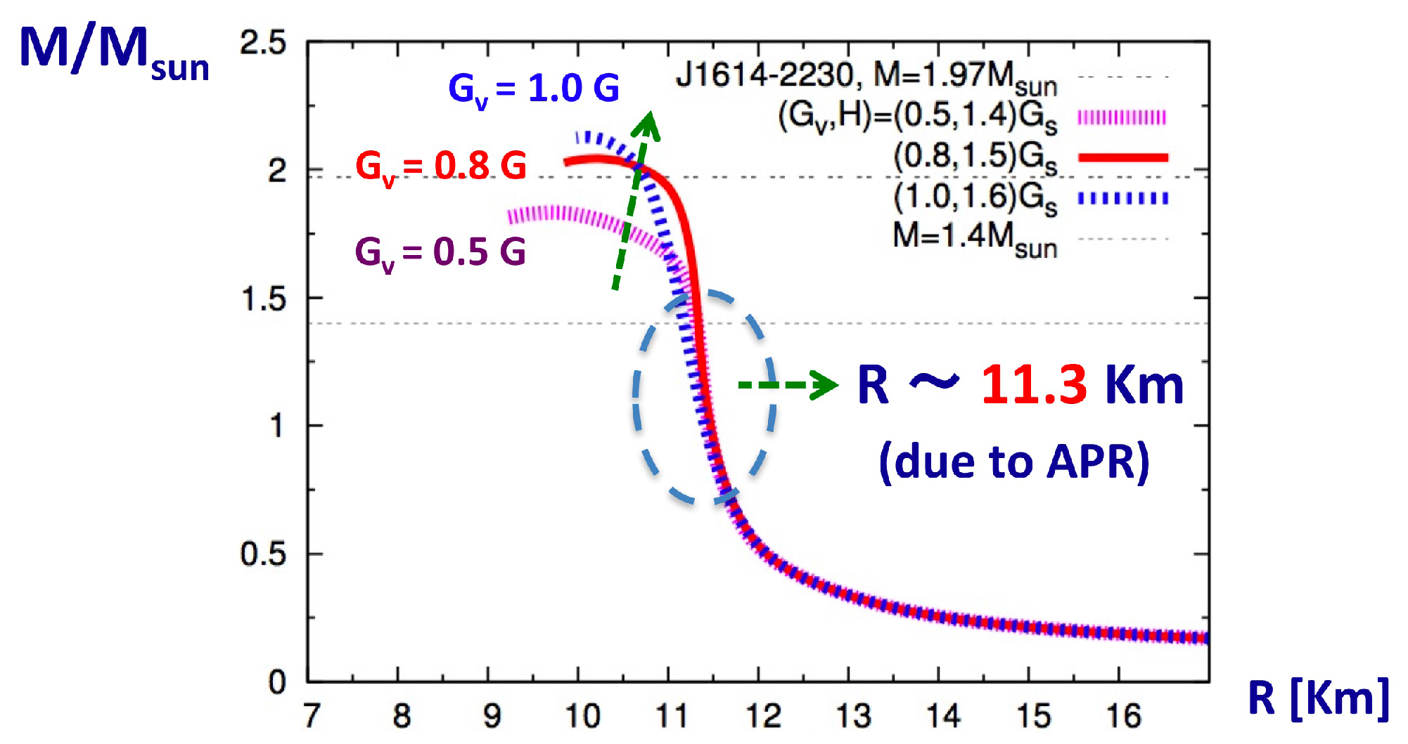
Figure 6.
The speed of sound square around the finite temperature crossover from hadron resonance gas to quark gluon plasma, on the possible first order chiral restoration line, and around the possible low temperature crossover from hadron to quark matter. While the finite temperature crossover has a dip in , the low temperature crossover has a peak.

Figure 7.
The phase diagram for gauged-Higgs model with the fixed Higgs amplitudes, in the 1/gs − |φ| plane. At large coupling, the confining and Higgs phases are smoothly connected.
Figure 7.
The phase diagram for gauged-Higgs model with the fixed Higgs amplitudes, in the 1/gs − |φ| plane. At large coupling, the confining and Higgs phases are smoothly connected.

© 2018 by the author. Licensee MDPI, Basel, Switzerland. This article is an open access article distributed under the terms and conditions of the Creative Commons Attribution (CC BY) license (http://creativecommons.org/licenses/by/4.0/).
Share and Cite
MDPI and ACS Style
Kojo, T. QCD Equations of State in Hadron–Quark Continuity. Universe 2018, 4, 42. https://doi.org/10.3390/universe4020042
AMA Style
Kojo T. QCD Equations of State in Hadron–Quark Continuity. Universe. 2018; 4(2):42. https://doi.org/10.3390/universe4020042
Chicago/Turabian StyleKojo, Toru. 2018. "QCD Equations of State in Hadron–Quark Continuity" Universe 4, no. 2: 42. https://doi.org/10.3390/universe4020042
Note that from the first issue of 2016, this journal uses article numbers instead of page numbers. See further details here.