Near-Horizon Geodesics for Astrophysical and Idealised Black Holes: Coordinate Velocity and Coordinate Acceleration


1
Department of Mathematics and Computer Science, Faculty of Science, Chulalongkorn University, Bangkok 10330, Thailand
2
Faculty of Science, Chandrakasem Rajabhat University, Bangkok 10900, Thailand
3
School of Mathematics and Statistics, Victoria University of Wellington, P.O. Box 600, Wellington 6140, New Zealand
*
Author to whom correspondence should be addressed.
Universe 2018, 4(6), 68; https://doi.org/10.3390/universe4060068
Submission received: 1 April 2018
/
Revised: 23 May 2018
/
Accepted: 24 May 2018
/
Published: 28 May 2018
(This article belongs to the Special Issue Gravity, Black Holes and Cosmology XXI)
Abstract
:Geodesics (by definition) have an intrinsic 4-acceleration zero. However, when expressed in terms of coordinates, the coordinate acceleration can very easily be non-zero, and the coordinate velocity can behave unexpectedly. The situation becomes extremely delicate in the near-horizon limit—for both astrophysical and idealised black holes—where an inappropriate choice of coordinates can quite easily lead to significant confusion. We shall carefully explore the relative merits of horizon-penetrating versus horizon-non-penetrating coordinates, arguing that in the near-horizon limit the coordinate acceleration is best interpreted in terms of horizon-penetrating coordinates.
Keywords:
geodesic equation; coordinate velocity; coordinate acceleration; horizon-penetrating coordinates; horizon-non-penetrating coordinatesPACS:
04.20.-q; 04.70.-s; 04.70.Bw; 02.40.Hw
1. Introduction
Coordinate dependence in general relativity is a topic that continues to cause confusion to this day, despite over 100 years of work on this issue. (For a variety of articles, both pro and con, both published and unpublished, see [1,2,3,4,5,6,7,8,9,10,11,12,13,14]. For two recent overviews, see [15,16]). The situation is particularly acute in the immediate vicinity of any horizon that might be present, whether it be for an astrophysical or an idealised (mathematical) black hole, where an inappropriate choice of coordinates can needlessly add to the confusion. Indeed, while horizons are often associated with coordinate singularities, these coordinate singularities are a property of the coordinate patch, not the spacetime geometry, and these coordinate singularities can quite easily go away with a different choice of coordinates. For astrophysical black holes, as opposed to maximally analytically extended idealised black holes, one still trusts the usual Einstein equations in the domain of outer communication—and down to any inner horizon that might be present. Similarly for the black holes arising from numerical simulations, which are key to modelling the astrophysical black holes of direct observational interest, one typically calculates down to some region inside the outer horizon, but well above the singular region, relying on the usual idealised picture for near-(outer)-horizon physics. Finally, for semi-classical black holes, as long as the quantum fields are in the Unruh vacuum state, the near-horizon geometry in the vicinity of the future horizon is qualitatively similar to that in classical general relativity.
In short, the black holes of observational interest in astronomy and cosmology can be adequately represented, at least in the domain of outer communication and down to any inner horizon that might be present, by the idealised Schwarzschild and Kerr spacetimes—and analysis of the near-horizon physics can adequately be performed using the classical Schwarzschild and Kerr spacetimes. In fact, it is very useful to distinguish:
- Horizon-penetrating coordinates—these coordinate systems are regular as one crosses the horizon (for example, Painleve–Gullstrand coordinates, Kerr–Schild coordinates, and variants thereof).
- Horizon-non-penetrating coordinates—these coordinate systems are singular as one crosses the horizon (for example, the Schwarzschild curvature coordinates, isotropic coordinates, and variants thereof).
The horizon-non-penetrating coordinates are simpler for some purposes (the metric is typically diagonal), but are ill-behaved in the immediate vicinity of the horizon. In contrast horizon-penetrating coordinates are better behaved in the immediate vicinity of the horizon, but the metric is typically non-diagonal, and the asymptotic behaviour may sometimes be more subtle than expected. We shall work through a number of examples illustrating the dangers and the pitfalls.
Consider for instance the Schwarzschild geometry—this is a very well-known spacetime since it was the first known exact solution to the (vacuum) Einstein field equations [17]. It is certainly of direct physical relevance—the spacetime geometry exterior to the sun and that exterior to slowly-rotating astrophysical black holes can be well-approximated by the Schwarzschild geometry. Perhaps the simplest form of the Schwarzschild spacetime is the Hilbert form expressed in terms of (what are now known as) Schwarzschild curvature coordinates [18,19,20]
There is a coordinate singularity at , see for instance [21,22,23,24,25,26,27,28,29,30], making this representation horizon-non-penetrating [31]. It is easy to see that in these coordinates the radial geodesics “pile up” at , never (in these coordinates) crossing the horizon. In fact, for any radial incoming geodesic, as one approaches the horizon.
Taking into account the Killing conservation law for the energy, we shall soon see that, even for infalling particles, sufficiently close to the horizon, though not at the horizon itself. However, this near-horizon phenomenon is a coordinate artefact; the behaviour can be very different in other coordinates. Despite this, some researchers are now (even in 2018) completely misinterpreting this coordinate artefact and asserting that “gravity becomes repulsive near the horizon”. This claim is, at best, a gross misinterpretation of the actual situation. (For specific examples of this particular confusion, see particularly [1,3,4,5,6,9,10,11,12,13]. For partial antidotes, see [7,8,14]. For a somewhat different sort of coordinate confusion, mistaking white holes for black holes, see [2].)
Below, we shall show that the coordinate acceleration near horizons is, in horizon-penetrating coordinates, (such as the Painleve–Gullstrand [32,33,34,35,36,37,38,39,40] or Kerr–Schild [21,24,27,28,29,40] coordinates), much easier to understand. We shall then wrap up with some generic comments regarding arbitrary horizon-penetrating coordinate systems [41,42,43,44].
We shall use letters from the beginning of the Roman alphabet (a, b, c, d, …) for spacetime indices, (see for instance Wald [22], or Hobson–Efstathiou–Lasenby [23]). Whenever there is a clearly defined time coordinate t, we shall use letters from the middle of the Roman alphabet (i, j, k, l, …) for the remaining spatial indices. We reserve the notation and for derivatives with respect to the time coordinate t.
2. Geodesic Equation
Consider the geodesic equation in non-affine-parameterised form:
This part of the analysis works equally well for timelike or null geodesics. Assume the zero’th coordinate is timelike, at least outside any horizon that might be present. That is, take . We can then choose the coordinate t to be a non-affine parameter for the geodesic. The geodesic equation separates into
The first of these equations implies
The second equation then becomes
This is still very general. Let us now specialize to spherical symmetry, taking
Then the radial geodesics are given by
That is,
Finally, regrouping, we see
Note that the “coordinate acceleration” is cubic in the “coordinate velocity” . This effect is certainly real if perhaps naively unexpected. (This effect is also manifestly coordinate-dependent.)
3. Killing Conservation Law for Energy: Coordinate Velocity
In all the situations we will be interested in, there is a timelike Killing vector (timelike outside any horizon that may be present), and there is no real loss of generality in taking the t coordinate to be compatible with that Killing vector; so . (That is, we choose coordinates to manifestly respect the time-translation Killing symmetry.) However, then any timelike geodesic with 4-velocity is subject to the energy conservation law
where is a constant, effectively the energy per unit rest mass. Observe that corresponds to dropping a particle at rest from spatial infinity; corresponds to dropping a moving particle from spatial infinity; corresponds to a gravitationally bound particle, dropped at rest from some finite radius. In fact, in an asymptotically flat spacetime, , where is the “coordinate velocity at infinity.” In spherical symmetry, this Killing conservation law can be written as
That is,
Even more explicitly,
This is quadratic in , with a general solution
Physically, the situation is this: If one drops a particle from some initial position with initial coordinate velocity , then one can calculate the energy from Equation (11) and subsequently extract at general positions r from Equation (15).
Formally, null geodesics can be viewed as the limit of this formalism. This is most easily seen from Equations (13) or (14), which in the limit imply
However, this is exactly the condition that the radial curve is a null curve. In this null limit, one sees that the Killing conservation law becomes
Two special cases are of particular interest:
- In coordinate charts where the metric is diagonal, (for example, the Schwarzschild curvature coordinates or isotropic coordinates), we have . Therefore, for timelike geodesics,As long as we are primarily interested in dropping (infalling) particles, we must choose the negative root and setIn the null limit (), this simplifies considerably and becomes
- In contrast, in coordinate charts where the metric satisfies , (for example, the Painleve–Gullstrand coordinates or Kerr–Schild coordinates), for timelike geodesics, we haveAs long as we are primarily interested in dropping (infalling) particles, we can safely choose the negative root and setNote that in order to keep real, while always, so choosing the negative root selects the ingoing geodesic.In the null limit (), this simplifies considerably and becomes
Let us now apply these quite general considerations to study the fixed-energy coordinate acceleration.
4. Coordinate Acceleration
For a dropped (timelike trajectory) particle, the coordinate acceleration at arbitrary radius is thus an interplay between the geodesic equation
and the Killing-induced coordinate velocity equation
Combining these results, we would get something of the general form
where is some explicit but coordinate-dependent function. Note that we could always use the chain rule to write . This serves as a consistency check, and side-steps the geodesic equation, but when doing so, one loses information regarding the coordinate velocity dependence of the coordinate acceleration. We shall now give a few examples of this phenomenon, focusing particularly on near-horizon behaviour.
5. Example: Schwarzschild Geometry
The Schwarzschild spacetime geometry is perhaps the pre-eminent example of an exact solution in general relativity [17,18,19,20,21,24,25,26,27]. As specific examples of near-horizon behaviour for the coordinate velocity and coordinate acceleration , let us consider the Schwarzschild spacetime in four commonly occurring coordinate systems [28,29,30,32,33,34,35,36]: Schwarzschild curvature coordinates, isotropic coordinates, Painleve–Gullstrand coordinates, and Kerr–Schild coordinates.
5.1. Schwarzschild Curvature Coordinates
The Schwarzschild geometry in Schwarzschild curvature coordinates is described by
It is easy to calculate the Christoffel symbols and to verify that the geodesic equation implies
This can be rewritten as
This gives the coordinate acceleration in terms of the Newtonian value , modified by relativistic corrections—due to both spacetime geometry and the local coordinate velocity. Furthermore, this already demonstrates (working in terms of r and ) that changes sign at the critical coordinate velocities given by
At large r (that is, weak fields), this sign flip takes place at ; this is mildly relativistic but certainly not ultra-relativistic. (In fact, this sign flip takes place for both ingoing and outgoing geodesics.) Furthermore, from the Killing conservation equation, we deduce
In particular at the horizon , and at spatial infinity, we see for fixed . Combining these geodesic and Killing results
Note that (for fixed ), the coordinate acceleration goes through zero and changes sign at the critical values of r given by
(In fact, this sign flip takes place for both ingoing and outgoing geodesics.) In particular, at the horizon for fixed .
For a time-like particle dropped at rest from spatial infinity (), this simplifies to
(Note that asymptotically , and , as expected from the Newtonian limit.)
Oddly enough (in this particular coordinate system), the coordinate acceleration switches sign at , the location of the innermost stable circular orbit (ISCO); this is a coincidence, not anything fundamental.
For a light-like particle (), this simplifies to
(Note that a photon can have non-trivial coordinate velocity and non-zero coordinate acceleration even if its physical speed is always exactly equal to c. This is one of the reasons that the concepts of coordinate velocity and coordinate acceleration must be used with care and discretion.)
Now these particular observations are not new, dating back (at least) to Hilbert in 1915 and the mid-1920s [18,19,20]. (It must be emphasised that Hilbert’s comments have subsequently been grossly misinterpreted by some of the later commentators on this topic.) (See particularly [1,3,4,5,6,9,10,11,12,13]. For partial antidotes, see [7,8,14]. For a different sort of coordinate confusion (mistaking white holes for black holes) see [2].) What is new in the current discussion is that we will now put these issues into a wider context emphasising the extent to which these results are simply coordinate artefacts.
5.2. Isotropic Coordinates
The Schwarzschild geometry in isotropic coordinates is described by [21]
Compared to Schwarzschild curvature coordinates, only the meaning of the r coordinate has changed. Indeed,
(In these isotropic coordinates, the horizon is now at .)
The Christoffel symbols are easily calculated and the geodesic equation becomes
This can also be recast as
This already demonstrates (working in terms of r and ) that changes sign at the critical coordinate velocities
At large r, (i.e., weak fields), this sign flip takes place at ; this is mildly relativistic but certainly not ultra-relativistic. (In the weak-field limit, the Schwarzschild curvature coordinates and the isotropic coordinates asymptotically approach each other.)
From the Killing conservation equation, since the metric in isotropic coordinates is diagonal, we deduce
This implies
Note that, at the horizon, now located at , we again have , while at spatial infinity we again see at fixed energy. Combining these results, for a dropped particle (of fixed energy ), we have
Note that the coordinate acceleration goes through zero and (apart from the trivial zero at ) changes sign at the critical values of r given by solving the cubic equation
For a particle dropped at rest from spatial infinity (), this simplifies to
with the (non-trivial) zeros of coordinate acceleration determined by
(Though not entirely obvious, it is easy to check that, at large distances , as expected from the Newtonian limit. It is more obvious that at large distances . In isotropic coordinates, the ISCO is at , which is not where ; that these two locations coincided in curvature coordinates is merely a coincidence.)
For null geodesics (), we have
5.3. Painleve–Gullstrand Coordinates
The Schwarzschild geometry in Painleve–Gullstrand coordinates is described by [32,33,34,35,36]
where the Painleve–Gullstrand time coordinate is given in terms of the Schwarzschild time coordinate by
Note in particular that .
It is easy to calculate the Christoffell symbols and verify that, in these coordinates, the radial geodesic equation becomes
We can rewrite this as
Viewed as a function of , this flips sign at the critical coordinate velocity
which is always positive outside the horizon. (This actually implies that factorizes as follows: , where the quadratic has no real zeroes. Unfortunately, the specific form of the quadratic is too messy to be illuminating.)
In view of the fact that, in these coordinates , the general Killing-induced result for the coordinate velocity simplifies to
Thence
This can also be written as
At the horizon, , we have
Therefore, we see that the ingoing geodesic crosses the horizon with finite coordinate velocity
while the outgoing geodesic crosses the horizon with coordinate velocity zero. (Note that can easily exceed unity; this is just a coordinate speed, not a physical speed.) This makes it clear that, for a dropped particle, we should take the negative root in so that
Combining these results, for a dropped particle (fixed energy ), we have
For a timelike particle dropped at rest from spatial infinity ( = 1), this simplifies quite drastically to yield
(The fact that in this particular situation the Painleve–Gullstrand coordinate system exactly reproduces the Newtonian result is one of the many reasons that the Painleve–Gullstrand coordinate system is so useful.)
Note that for the (ingoing) coordinate acceleration is extremely simple, and always negative. In fact, the coordinate acceleration is finite at horizon crossing .
For an infalling light-like particle (), this again simplifies quite drastically to yield
Note that for the (ingoing) coordinate acceleration is relatively simple, and always negative. In fact, the coordinate acceleration is finite at horizon crossing . (The situation for Painleve–Gullstrand coordinates is ultimately so simple that graphs are not needed.)
5.4. Kerr–Schild Coordinates
That is,
Note in particular that .
The Christoffel symbols are easily calculated and in these coordinates the radial geodesic equation becomes
It may be better to rewrite this as follows:
This factorizes
As a function of , we see that flips sign at the critical coordinate velocity
This is always positive, and less than 1/2, outside the horizon.
In view of the fact that in these coordinates , the general Killing-induced result for the coordinate velocity simplifies to
Thence
At the horizon
Therefore, the ingoing geodesic crosses the horizon with finite coordinate velocity
while the outgoing geodesic crosses the horizon with coordinate velocity zero. This makes it clear that, for a dropped particle, we should take the negative root in .
Combining these results, for a dropped (ingoing) particle (fixed energy ), we have
For unbound particles (), this is negative real everywhere, both outside and inside the horizon—in fact, all the way down to . For the coordinate acceleration,
At the horizon, , we have
a finite inward coordinate acceleration.
For a timelike particle dropped at rest from spatial infinity ( = 1), this simplifies to
(Note that asymptotically , as expected from the Newtonian limit.) Furthermore,
Note that the coordinate acceleration and the coordinate velocity are both always negative. We can also factorize this as
We can see that when approaching the horizon, at fixed , we have
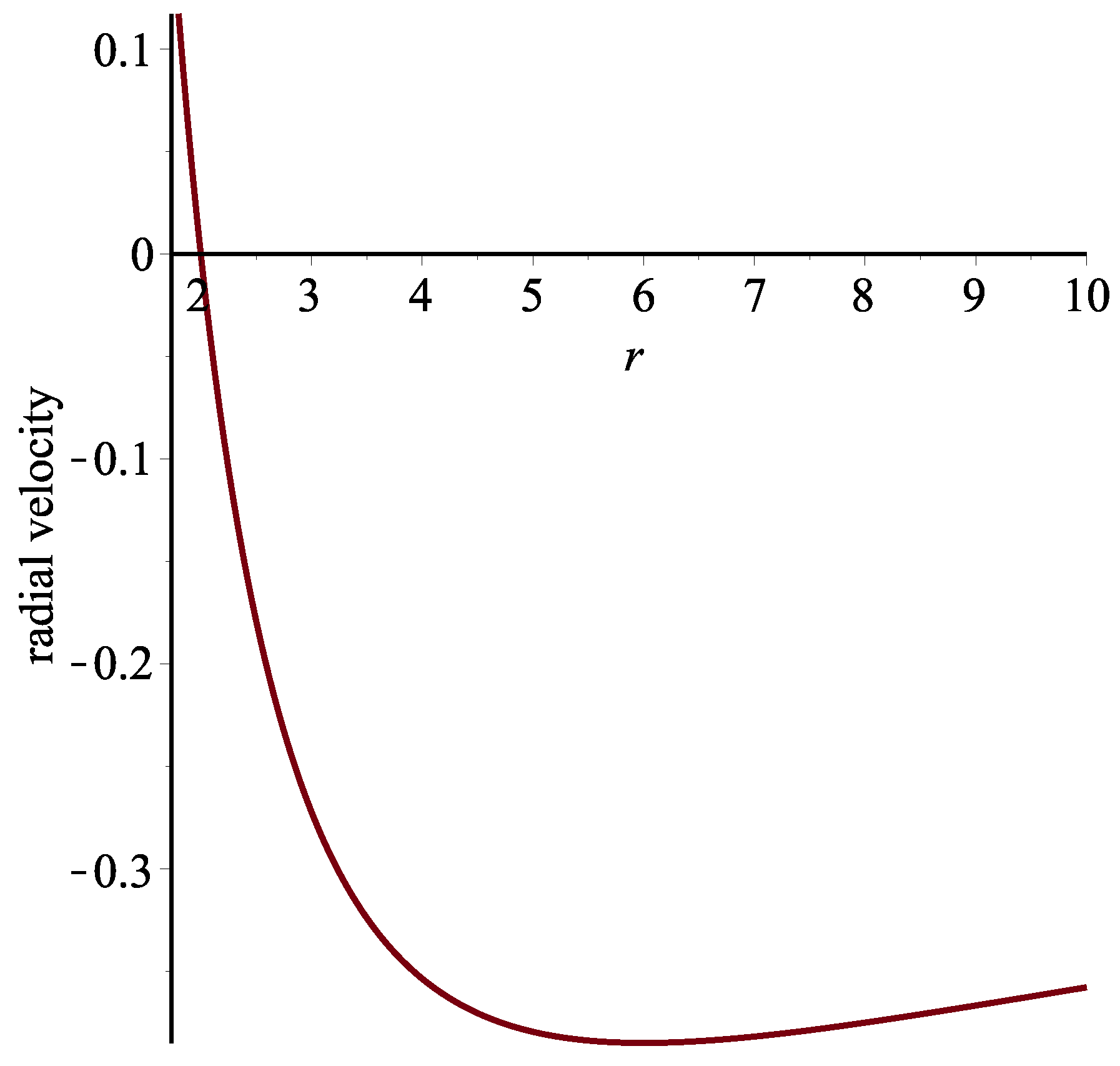
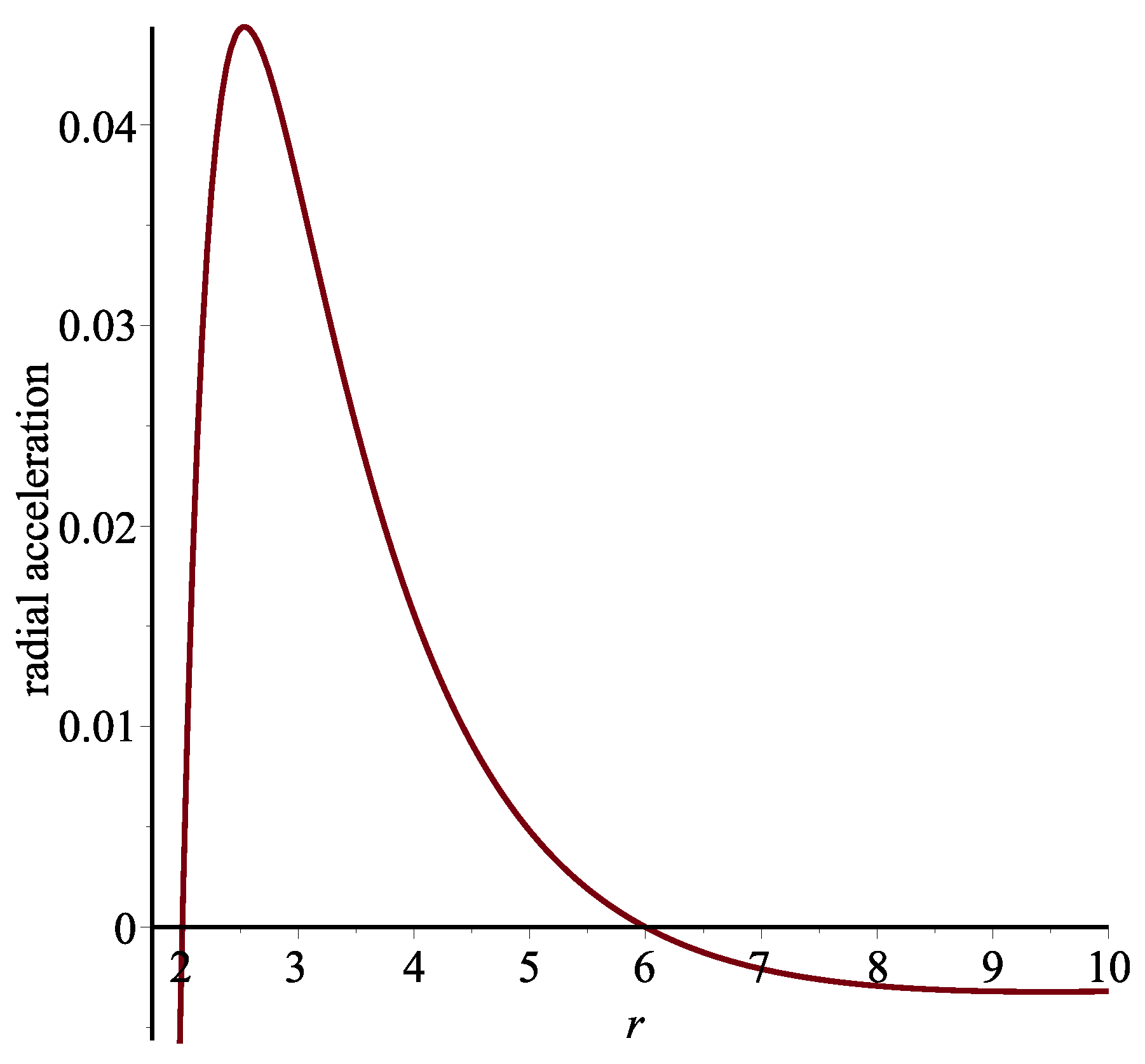
The radial coordinate velocity and radial coordinate acceleration are plotted as shown in Figure 9 and Figure 10, respectively.
Finally, note that for a light-like particle () in Kerr–Schild coordinates, we have the very drastic simplification
(Therefore, in Kerr–Schild coordinates, ingoing photons happen to have coordinate acceleration zero. This is one reason Kerr–Schild coordinates are popular. For this particular case, a figure would be entirely superfluous.)
6. Conclusions
Now that we have seen some examples of what happens to near-horizon geodesics in various coordinate systems, let us attempt to draw some general inferences. While the specific computations in this article have been carried out for the Schwarzschild geometry, this is known to be a good approximation for slowly rotating astrophysical black holes, and for numerical simulations of black holes, and even for semi-classical black holes in the Unruh quantum vacuum—so the overall conclusions are generic to a wide class of physically and observationally interesting black holes.
The most obvious conclusion we can draw is that the coordinate velocity, and coordinate acceleration, are (quite naturally) extremely coordinate-dependent, and that no general physical conclusions can be drawn from the magnitude of the coordinate velocity ( can easily exceed unity) or the sign of the coordinate acceleration . Claims that gravity in general relativity is “repulsive” at high speeds and/or near the horizon are at best disingenuous—they are merely misinterpretations of coordinate artefacts. For a fixed spacetime, by suitably choosing the coordinate system we can easily make or at horizon crossing. For a fixed spacetime, by suitably choosing the coordinate system we can easily make the coordinate acceleration either positive or negative just prior to horizon crossing. Indiscriminately mixing general relativistic and Newtonian concepts is dangerous and misleading.
The major distinction we have seen in the specific examples we explored was in the difference between horizon-penetrating and horizon-non-penetrating coordinates. There are good physical and mathematical reasons for this. In horizon-non-penetrating coordinates geodesics (essentially by definition) pile up at the horizon and do not cross it—in coordinates of this type first increases as one falls inwards, but then has to go to zero at the horizon. This implies that must have a maximum where and hence . Thence, regions where the coordinate acceleration is positive are unavoidable in horizon-non-penetrating coordinates. In contrast, horizon-penetrating coordinates are much better behaved when studying near horizon physics, with the coordinate velocity and coordinate acceleration being non-zero and finite at horizon crossing.
Author Contributions
All three authors contributed equally to this work.
Funding
This project was funded by the Ratchadapisek Sompoch Endowment Fund, Chulalongkorn University (Sci-Super 2014-032), by a grant for the professional development of new academic staff from the Ratchadapisek Somphot Fund at Chulalongkorn University, by the Thailand Research Fund (TRF), and by the Office of the Higher Education Commission (OHEC), Faculty of Science, Chulalongkorn University (RSA5980038). PB was additionally supported by a scholarship from the Royal Government of Thailand. TN was also additionally supported by a scholarship from the Development and Promotion of Science and Technology talent project (DPST). MV was supported by the Marsden Fund, via a grant administered by the Royal Society of New Zealand.
Conflicts of Interest
The authors declare no conflicts of interest.
References
- McGruder, C.H. Acceleration of particles to high energy via gravitational repulsion in the Schwarzschild field. Astropart. Phys. 2017, 86, 18–20. [Google Scholar] [CrossRef]
- Guerreiro, T.; Monteiro, F. Light geodesics near an evaporating black hole. Phys. Lett. A 2015, 379, 2441–2444. [Google Scholar] [CrossRef]
- Felber, F. Test of relativistic gravity for propulsion at the Large Hadron Collider. AIP Conf. Proc. 2010, 1208, 247–260. [Google Scholar]
- Felber, F.S. Exact relativistic ‘antigravity’ propulsion. AIP Conf. Proc. 2006, 813, 1374–1381. [Google Scholar]
- Mashhoon, B. Beyond gravito-electro-magnetism: Critical speed in gravitational motion. Int. J. Mod. Phys. D 2005, 14, 2025–2037. [Google Scholar] [CrossRef]
- Krori, K.D.; Barua, M. Gravitational Repulsion by Kerr and Kerr–Newman Black Holes. Phys. Rev. D 1985, 31, 3135–3139. [Google Scholar] [CrossRef]
- Spallicci, A.D.A.M. Comment on “Acceleration of particles to high energy via gravitational repulsion in the Schwarzschild field” [Astropart. Phys. 86 (2017) 18–20]. Astropart. Phys. 2017, 94, 42–43. [Google Scholar] [CrossRef]
- Spallicci, A.D.A.M.; Ritter, P. A fully relativistic radial fall. Int. J. Geom. Meth. Mod. Phys. 2014, 11, 1450090. [Google Scholar] [CrossRef] [Green Version]
- Berkahn, D.L.; Chappell, J.M.; Abbott, D. Velocity dependence of point masses, moving on timelike geodesics, in weak gravitational fields. arXiv, 2017; arXiv:1708.09725. [Google Scholar]
- Berkahn, D.L.; Chappell, J.M.; Abbott, D. Hilbert’s forgotten equation of velocity dependent acceleration in a gravitational field. arXiv, 2017; arXiv:1708.0143. [Google Scholar]
- Célérier, M.-N.; Santos, N.O.; Satheeshkumar, V.H. Can gravity be repulsive? arXiv, 2016; arXiv:1606.08300. [Google Scholar]
- Felber, F. Comment on “Reversed gravitational acceleration…”, arXiv:1102.2870v2. arXiv, 2011; arXiv:1111.6564. [Google Scholar]
- Loinger, A.; Marsico, T. On Hilbert’s gravitational repulsion (A historical Note). arXiv, 2009; arXiv:0904.1578. [Google Scholar]
- Ohanian, H.C. Reversed Gravitational Acceleration for High-speed Particles. arXiv, 2011; arXiv:1102.2870. [Google Scholar]
- Iorio, L. 100 Years of Chronogeometrodynamics: The Status of the Einstein’s Theory of Gravitation in Its Centennial Year. Universe 2015, 1, 38–81. [Google Scholar] [CrossRef]
- Debono, I.; Smoot, G.F. General Relativity and Cosmology: Unsolved Questions and Future Directions. Universe 2016, 2, 23. [Google Scholar] [CrossRef]
- Schwarzschild, K. On the gravitational field of a mass point according to Einstein’s theory. Sitzungsber. Preuss. Akad. Wiss. Phys. Math. 1916, 1916, 189–196. [Google Scholar]
- Hilbert, D. Die Grundlagen der Physik. (Erste Mitteilung.). Nachrichten von der Gesellschaft der Wissenschaften zu Göttingen, Mathematisch-Physikalische Klasse 1915, 1915, 395–408. [Google Scholar]
- Hilbert, D. Die Grundlagen der Physik. (Zweite Mitteilung). Nachrichten von der Gesellschaft der Wissenschaften zu Göttingen, Mathematisch-Physikalische Klasse 1917, 1917, 53–76. [Google Scholar]
- Hilbert, D. Die Grundlagen der Physik. Math. Ann. 1924, 92, 1–32. [Google Scholar] [CrossRef]
- Misner, C.W.; Thorne, K.S.; Wheeler, J.A. Gravitation; W. H. Freeman and Company: San Francisco, CA, USA, 1973. [Google Scholar]
- Wald, R.M. General Relativity; University of Chicago Press: Chicago, IL, USA, 1984. [Google Scholar]
- Hobson, M.P.; Efstathiou, G.P.; Lasenby, A.N. General Relativity: An Introduction for Physicists; Cambridge University Press: Cambridge, UK, 2006. [Google Scholar]
- Stephani, H.; Kramer, D.; MacCallum, M.; Hoenselaers, C.; Herlt, E. Exact Solutions of Einstein’s Field Equations; Cambridge University Press: Cambridge, UK, 2002. [Google Scholar]
- Parry, A.R. A Survey of Spherically Symmetric Spacetimes. Anal. Math. Phys. 2014, 4, 333–375. [Google Scholar] [CrossRef]
- Muller, T.; Grave, F. Catalogue of Spacetimes. arXiv, 2009; arXiv:0904.4184. [Google Scholar]
- Visser, M. Lorentzian Wormholes: From Einstein to Hawking; Springer: Woodbury, NY, USA, 1995. [Google Scholar]
- Martel, K.; Poisson, E. Regular coordinate systems for Schwarzschild and other spherical spacetimes. Am. J. Phys. 2001, 69, 476–480. [Google Scholar] [CrossRef]
- Lake, K. A Class of quasi-stationary regular line elements for the Schwarzschild geometry. arXiv, 1994; arXiv:gr-qc/9407005. [Google Scholar]
- Czerniawski, J. What is wrong with Schwarzschild’s coordinates? Concepts Phys. 2006, 3, 307–318. [Google Scholar]
- Fromholz, P.; Poisson, E.; Will, C.M. The Schwarzschild metric: It’s the coordinates, stupid. Am. J. Phys. 2014, 82, 295–300. [Google Scholar] [CrossRef]
- Painlevé, P. La mécanique classique et la theorie de la relativité. C. R. Acad. Sci. 1921, 173, 677–680. [Google Scholar]
- Gullstrand, A. Allgemeine Lösung des statischen Einkörper-problems in der Einsteinschen Gravitationstheorie. Ark. Mat. Astron. Fys. 1922, 16, 1–15. [Google Scholar]
- Visser, M. Acoustic propagation in fluids: An unexpected example of Lorentzian geometry. arXiv, 1993; arXiv:gr-qc/9311028. [Google Scholar]
- Visser, M. Acoustic black holes: Horizons, ergospheres, and Hawking radiation. Class. Quant. Gravity 1998, 15, 1767–1791. [Google Scholar] [CrossRef]
- Barceló, C.; Liberati, S.; Visser, M. Analogue gravity. Living Rev. Relativ. 2005, 8, 12. [Google Scholar] [CrossRef] [PubMed]
- Hamilton, A.J.S.; Lisle, J.P. The River model of black holes. Am. J. Phys. 2008, 76, 519–532. [Google Scholar] [CrossRef]
- Visser, M. Heuristic approach to the Schwarzschild geometry. Int. J. Mod. Phys. D 2005, 14, 2051–2067. [Google Scholar] [CrossRef]
- Finch, T.K. Coordinate families for the Schwarzschild geometry based on radial timelike geodesics. Gen. Relativ. Gravit. 2015, 47, 56. [Google Scholar] [CrossRef]
- Rosquist, K. A moving medium simulation of Schwarzschild black hole optics. Gen. Relativ. Gravit. 2004, 36, 1977–1982. [Google Scholar] [CrossRef]
- Wiltshire, D.L.; Visser, M.; Scott, S.M. (Eds.) The Kerr Spacetime: Rotating Black Holes in General Relativity; Cambridge University Press: Cambridge, UK, 2005. [Google Scholar]
- Visser, M. The Kerr spacetime: A brief introduction. arXiv, 2007; arXiv:0706.0622. [Google Scholar]
- Rosquist, K. A unifying coordinate family for the Kerr–Newman metric. Gen. Relativ. Gravit. 2009, 41, 2619–2632. [Google Scholar] [CrossRef]
- Rajan, D.; Visser, M. Cartesian Kerr–Schild variation on the Newman–Janis ansatz. Int. J. Mod. Phys. D 2017, 26, 1750167. [Google Scholar] [CrossRef]
Figure 1.
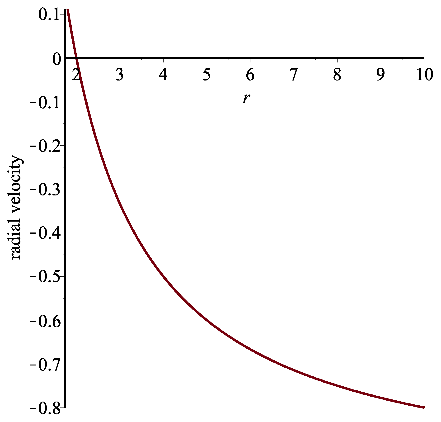
Behaviour of in the Schwarzschild geometry when using Schwarzschild curvature coordinates for and . Note the curve crosses the r axis only at , and the coordinate velocity is negative all the way from the horizon to spatial infinity.
Figure 1.
Behaviour of in the Schwarzschild geometry when using Schwarzschild curvature coordinates for and . Note the curve crosses the r axis only at , and the coordinate velocity is negative all the way from the horizon to spatial infinity.

Figure 2.
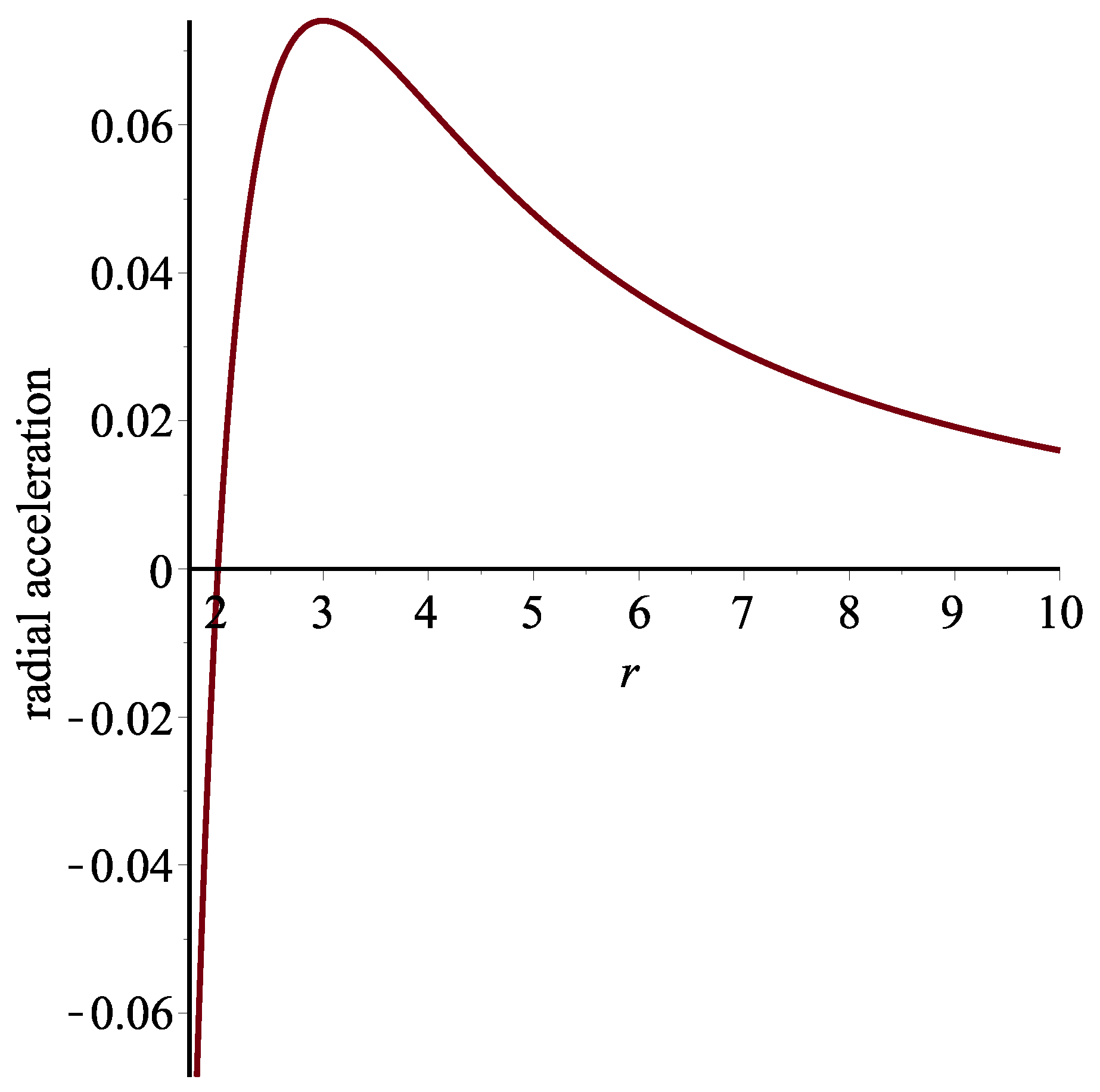
Behaviour of in the Schwarzschild geometry when using Schwarzschild curvature coordinates for and . Note the curve crosses the r axis at both and ; the coordinate acceleration is positive between the horizon and the ISCO.
Figure 2.
Behaviour of in the Schwarzschild geometry when using Schwarzschild curvature coordinates for and . Note the curve crosses the r axis at both and ; the coordinate acceleration is positive between the horizon and the ISCO.

Figure 3.
Behaviour of for null geodesics in the Schwarzschild geometry when using Schwarzschild curvature coordinates for and . Note the curve crosses the r axis only at , and the coordinate velocity is negative all the way from the horizon to spatial infinity.
Figure 3.
Behaviour of for null geodesics in the Schwarzschild geometry when using Schwarzschild curvature coordinates for and . Note the curve crosses the r axis only at , and the coordinate velocity is negative all the way from the horizon to spatial infinity.

Figure 4.
Behaviour of for null geodesics in the Schwarzschild geometry when using Schwarzschild curvature coordinates for and . Note the curve crosses the r axis only at , and the coordinate acceleration is positive all the way from the horizon to spatial infinity.
Figure 4.
Behaviour of for null geodesics in the Schwarzschild geometry when using Schwarzschild curvature coordinates for and . Note the curve crosses the r axis only at , and the coordinate acceleration is positive all the way from the horizon to spatial infinity.

Figure 5.
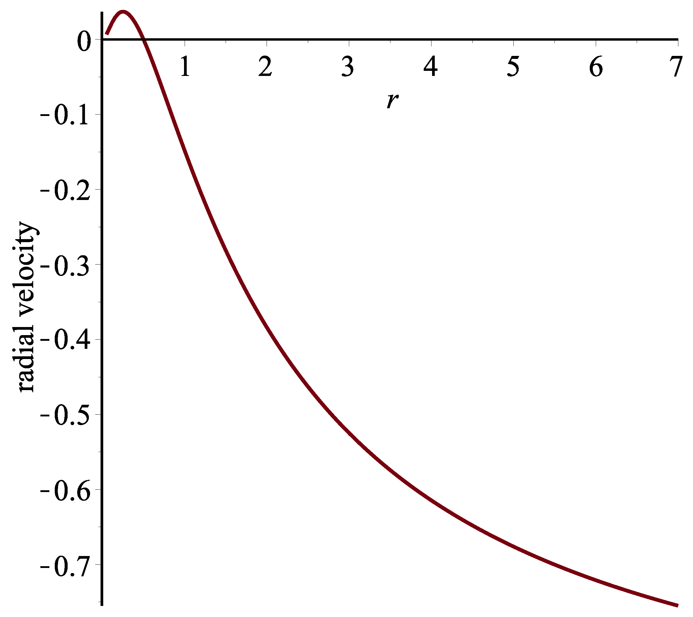
Behaviour of in the Schwarzschild geometry using isotropic coordinates for and . Note the coordinate velocity is negative all the way from the horizon (now at ) to spatial infinity.
Figure 5.
Behaviour of in the Schwarzschild geometry using isotropic coordinates for and . Note the coordinate velocity is negative all the way from the horizon (now at ) to spatial infinity.

Figure 6.
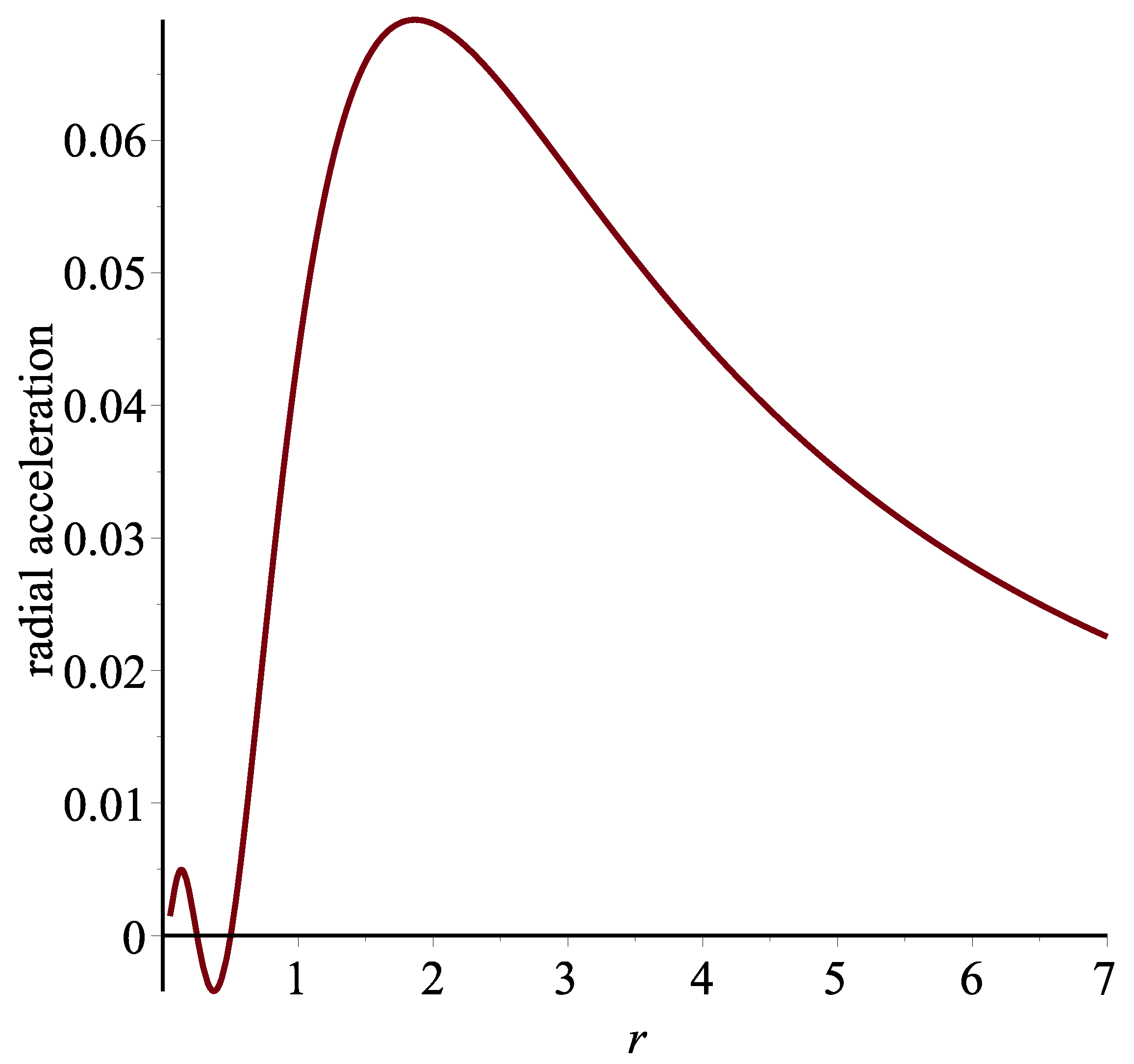
Behaviour of in the Schwarzschild geometry using isotropic coordinates for and . Note that the curve crosses the r axis both at and ; there is a third unphysical root at .
Figure 6.
Behaviour of in the Schwarzschild geometry using isotropic coordinates for and . Note that the curve crosses the r axis both at and ; there is a third unphysical root at .

Figure 7.
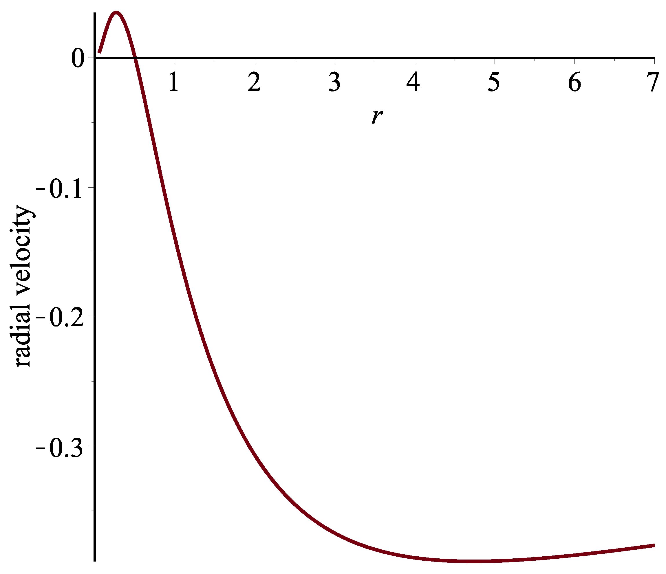
Behaviour of for null geodesics in the Schwarzschild geometry using isotropic coordinates for and . Note the coordinate velocity is negative all the way from the horizon (now at ) to spatial infinity.
Figure 7.
Behaviour of for null geodesics in the Schwarzschild geometry using isotropic coordinates for and . Note the coordinate velocity is negative all the way from the horizon (now at ) to spatial infinity.

Figure 8.
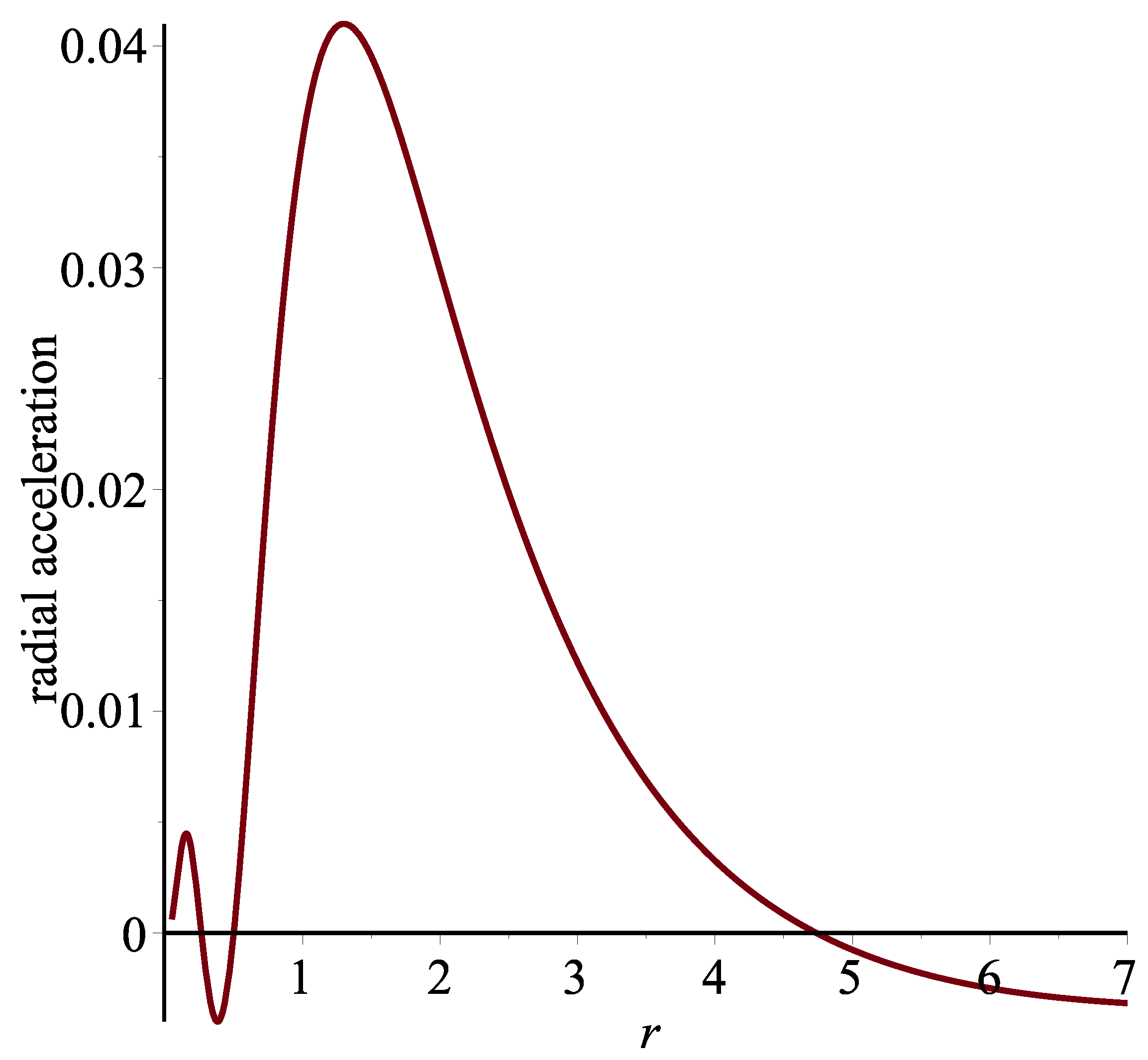
Behaviour of for null geodesics in the Schwarzschild geometry using isotropic coordinates for and . Note the horizon is now at ; there is an extra zero at . Note the coordinate acceleration is positive all the way from the horizon to spatial infinity.
Figure 8.
Behaviour of for null geodesics in the Schwarzschild geometry using isotropic coordinates for and . Note the horizon is now at ; there is an extra zero at . Note the coordinate acceleration is positive all the way from the horizon to spatial infinity.

Figure 9.
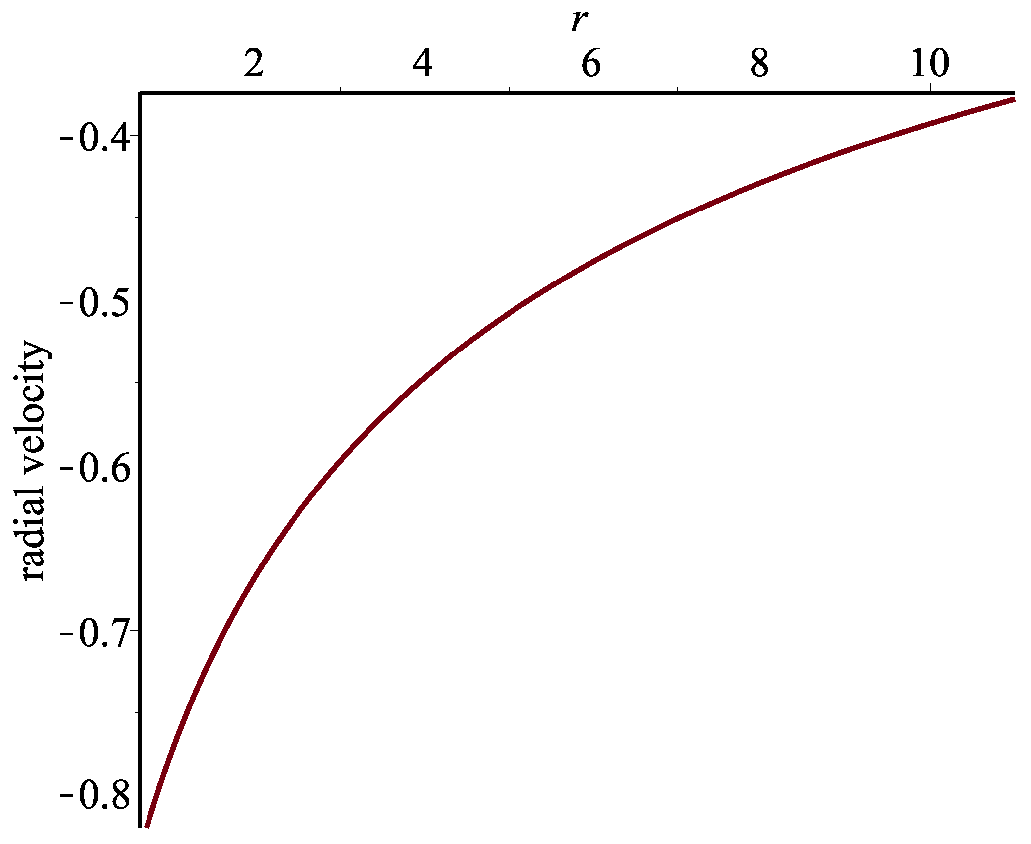
Behaviour of for the Schwarzschild geometry in Kerr–Schild coordinates for and . Note that the coordinate velocity at the horizon is and that the coordinate velocity remains negative between the horizon and spatial infinity.
Figure 9.
Behaviour of for the Schwarzschild geometry in Kerr–Schild coordinates for and . Note that the coordinate velocity at the horizon is and that the coordinate velocity remains negative between the horizon and spatial infinity.

Figure 10.
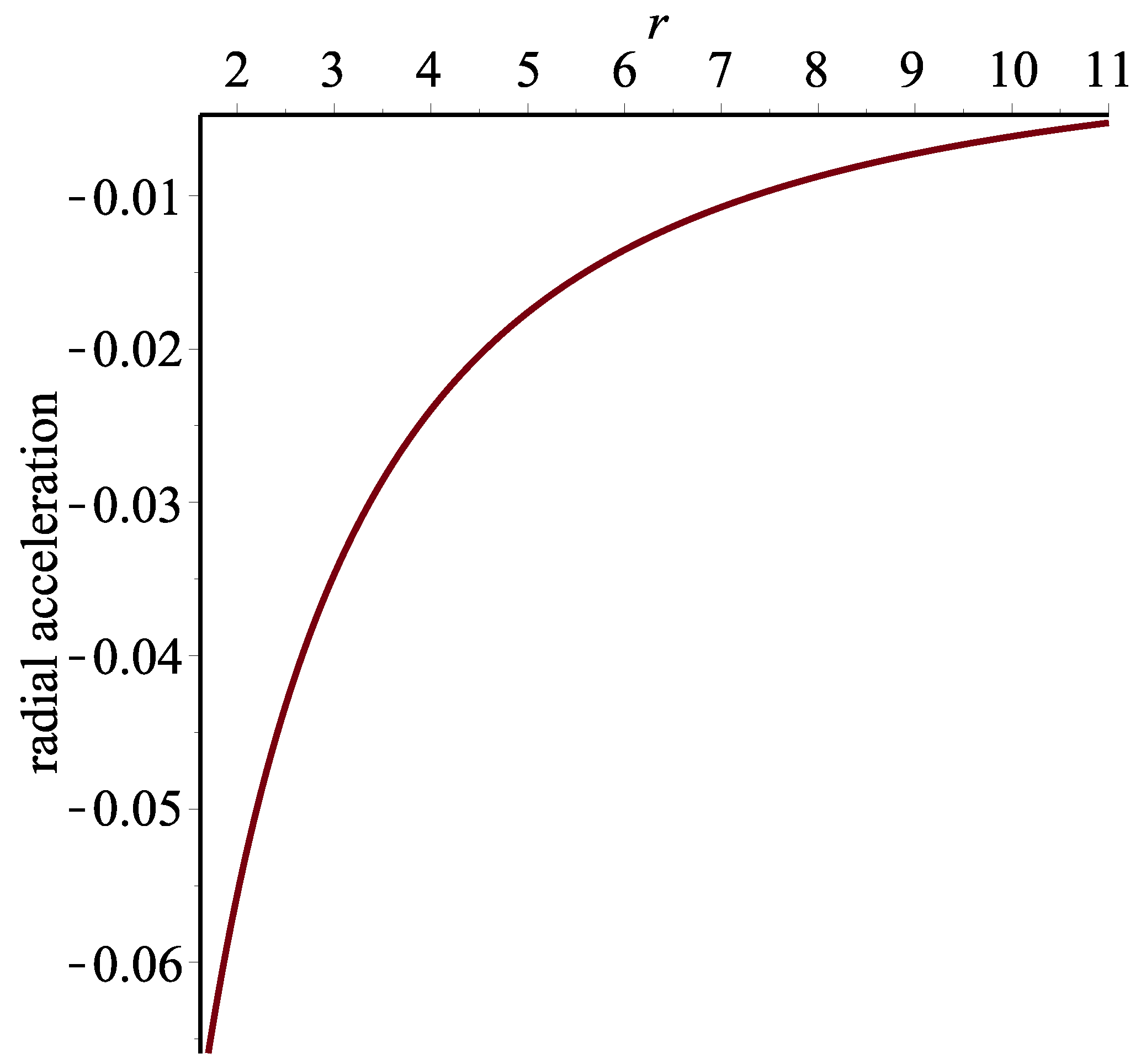
Behaviour of for the Schwarzschild geometry in Kerr–Schild coordinates for and . Note the coordinate acceleration remains negative between the horizon and spatial infinity.
Figure 10.
Behaviour of for the Schwarzschild geometry in Kerr–Schild coordinates for and . Note the coordinate acceleration remains negative between the horizon and spatial infinity.

© 2018 by the authors. Licensee MDPI, Basel, Switzerland. This article is an open access article distributed under the terms and conditions of the Creative Commons Attribution (CC BY) license (http://creativecommons.org/licenses/by/4.0/).
Share and Cite
MDPI and ACS Style
Boonserm, P.; Ngampitipan, T.; Visser, M. Near-Horizon Geodesics for Astrophysical and Idealised Black Holes: Coordinate Velocity and Coordinate Acceleration. Universe 2018, 4, 68. https://doi.org/10.3390/universe4060068
AMA Style
Boonserm P, Ngampitipan T, Visser M. Near-Horizon Geodesics for Astrophysical and Idealised Black Holes: Coordinate Velocity and Coordinate Acceleration. Universe. 2018; 4(6):68. https://doi.org/10.3390/universe4060068
Chicago/Turabian StyleBoonserm, Petarpa, Tritos Ngampitipan, and Matt Visser. 2018. "Near-Horizon Geodesics for Astrophysical and Idealised Black Holes: Coordinate Velocity and Coordinate Acceleration" Universe 4, no. 6: 68. https://doi.org/10.3390/universe4060068
Note that from the first issue of 2016, this journal uses article numbers instead of page numbers. See further details here.