Baryon Physics and Tight Coupling Approximation in Boltzmann Codes

1
Center for Gravitational Physics, Yukawa Institute for Theoretical Physics, Kyoto University, Kyoto 606-8502, Japan
2
Kavli Institute for the Physics and Mathematics of the Universe (WPI), The University of Tokyo, Institutes for Advanced Study, The University of Tokyo, Kashiwa, Chiba 277-8583, Japan
*
Author to whom correspondence should be addressed.
Universe 2020, 6(1), 6; https://doi.org/10.3390/universe6010006
Submission received: 25 November 2019
/
Revised: 27 December 2019
/
Accepted: 28 December 2019
/
Published: 31 December 2019
(This article belongs to the Section Cosmology)
Abstract
:We provide two derivations of the baryonic equations that can be straightforwardly implemented in existing Einstein–Boltzmann solvers. One of the derivations begins with an action principle, while the other exploits the conservation of the stress-energy tensor. While our result is manifestly covariant and satisfies the Bianchi identities, we point out that this is not the case for the implementation of the seminal work by Ma and Bertschinger and in the existing Boltzmann codes. We also study the tight coupling approximation up to the second order without choosing any gauge using the covariant full baryon equations. We implement the improved baryon equations in a Boltzmann code and investigate the change in the estimate of cosmological parameters by performing an MCMC analysis. With the covariantly correct baryon equations of motion, we find deviation for the best fit values of the cosmological parameters that should be taken into account. While in this paper, we study the CDM model only, our baryon equations can be easily implemented in other models and various modified gravity theories.
1. Introduction
Studies in modern cosmology heavily rely on cosmological linear perturbation theory [1,2]. To understand the evolution of these linear perturbations, Einstein’s equations are solved numerically at the linear order in perturbations around a homogeneous and isotropic background. These numerical solvers are often referred to as Boltzmann solvers or Boltzmann codes. There are several open-source linear Boltzmann solvers available, namely the Cosmic Linear Anisotropy Solving System (CLASS) [3], Code for Anisotropies in the Microwave Background (CAMB) [4], CMBEASY [5], CMBFAST [6], etc. Among them, CAMB and CLASS are maintained frequently. These codes provide us with a platform to test any theory against observations.appropriate.
To understand the nature of the dark sector of our universe, there are several future experiments planned, such as EUCLID [7], the Dark Energy Spectroscopic Instrument (DESI) [8], and Large Synoptic Survey Telescope (LSST) [9]. All these experiments focus on higher precision than the current dataset like Planck, for the estimate of cosmological parameters. In order to take full advantage of these experiments, the Boltzmann codes need to be precise enough, and any inconsistencies present in the implementation of the codes need to be fixed. Otherwise, theoretical predictions cannot be matched with the observations.
The first calculation of cosmological perturbation theory was performed by Lifshitz [10]. Later, Bardeen [11] and Kodama and Sasaki [1] fixed the gauge issues in the scalar sector. CMBFAST [6] makes use of the line-of-sight integration method to compute anisotropies, and their code was made publicly available. This could reduce the time for computation up to two times. There were two other Boltzmann codes available before, one developed by Sugiyama [12,13], based on gauge invariant formalism, and the other developed by White, based on the synchronous gauge [14,15,16]. CMBFAST is also based on the synchronous gauge. CMBEASY and CAMB are basically formulated based on CMBFAST. The Boltzmann equations in CMBFAST are taken from COSMIC [17], which is based on the seminal work by Ma and Bertschinger [18]. CLASS is also based on it, implemented in Newtonian and synchronous gauges.
However, in [18], there appeared to be at least three possible problems in the evolution equation for the baryon fluid.
- First, there is a gauge incompatibility, that is the equations break general covariance. In particular, the equations of motion in the Newtonian gauge and those in the synchronous gauge are not related to each other by a gauge transformation. This results in different physical outcomes for different gauge choices. The consequence is that it is not clear which gauge one should choose from the beginning to study baryons. This should not happen in a covariant theory, as a gauge choice merely represents a choice of coordinates and does not affect physical results.
- Second, it breaks the Bianchi identity. This aspect also leads to inconsistencies. For example, breaking the Bianchi identity implies that solving all components of the Einstein equations would lead in general to a solution that is not consistent with the conservation equation for the matter fields.
- Third, in the limit of no interaction between the baryon fluid and the photon gas, we have an equation of motion for the baryons in which the squared sound speed is present. It is difficult to understand the nature of this term with , as no known covariant action for matter would lead to such a term in the dynamical equation of motion.
As mentioned above, these equations are taken for code implementation in almost all existing Boltzmann solvers. We feel that in this era of precision cosmology, the Boltzmann solvers should have these issues fixed. These issues cause artificial deviations from general relativity. These problems appeared also in [15]. We find that there are terms missing at the order of in the baryon evolution equation. In this work, we derive the correct equations of motion for baryons from an action. The resulting equations are devoid of the above mentioned issues. We shall see that our new terms do not modify strongly the final results (and this is a bit reassuring); nonetheless, we believe our corrections are to be made for Boltzmann solvers, especially at early times, when the sound speed of the baryon fluid (though small) cannot be neglected completely.
In fact, in the regime before recombination, photons and baryons coupled to form a stiff baryon-photon fluid. Since, in this case, the equations for this photon-baryon fluid are numerically stiff, in order to study this regime, both CLASS and CAMB make use of the so-called tight coupling approximations. These were first developed by Peebles and Yu [19]. In [18], the authors developed this approximation up to the first order, and they further assumed (where , a is the scale factor, is the electron density, and is the Thomson cross-section) and (where is the speed of propagation for the baryon fluid). The full first order tight coupling approximation was implemented in [4] with an additional approximation, For CMBEASY, tight coupling approximation is calculated for the Newtonian gauge in which they considered terms beyond the first order [5]. CLASS developed both first order and second order tight coupling approximation without assuming any further assumptions like in COSMIC and CAMB. Several other authors have worked on the tight coupling approximation. For example, the tight coupling approximation up to the second order was implemented for the calculation in the synchronous gauge in [20]. An extension of the tight coupling approximation to second order in the perturbation was developed in [21]. The approximation depends on the baryon equations. Hence, also the approximation methods used to solve the baryon-photon system need to be revised.
In order to fix the covariance issues, we find it useful to understand the baryon physics, starting from a newly written Lagrangian, which up to a field redefinition is equivalent to the Schutz–Sorkin Lagrangian [22], which was studied also in [23,24] in the context of perfect fluids, with general equations of state. We then consider the baryon fluid as an ideal gas. This is in fact a gas model for non-relativistic particles with a non-zero speed of propagation, i.e., . This system then allows us to find covariant equations of motion for the perturbation variables (we also give an alternative derivation of the same set of equations based on the conservation of the stress-energy tensor). We find that there is an extra term of the order of in both the evolution of energy density and velocity perturbations for the baryon fluid. This fix solves all three problems mentioned above. We then use these new baryon equations of motion in order to derive the tight coupling approximation equations up to the second order. We implement these corrections for the baryon evolution, in the CLASS code. Finally, we make a parameter estimation for the CDM model with these new corrections, using the Monte Carlo sampler Monte Python [25,26]. We find that the new equations, solved by CLASS, give some deviations from the previous results, but for the parameter estimation of the model, such deviations are inside the statistical error bars (on the other hand, we do not know whether the deviation remains within the statistical error bars in other models and various modified gravity theories).
For the clarity of the reader, we would like to summarize the main difference between Ma and Bertschinger’s paper [18] and our paper. Ma and Bertschinger’s starting equations, i.e., Equations (29–30) (MB29–30) of [18], are compatible with ours, but are not ready to be implemented for baryons in Boltzmann codes. In fact, the equations that instead have been implemented in existing Boltzmann codes are different from ours and consequently incompatible with MB29–30. This is because the equations of motion used in existing Boltzmann codes, which correspond instead to Equations (66–67) of [18] (MB66–67), have some terms removed from the correct equations, which make them incompatible with MB29–30. In our code, we have instead implemented the correct equations of motion that are compatible with MB29–301.
Since the baryon equations of motion MB66–67 (the ones used in Boltzmann codes) are not compatible with MB29–30 (which instead follow from conservation of energy-momentum), they end up breaking general covariance. Therefore, MB66–67 equations describe a system, baryons, which does not satisfy the energy-momentum conservation.
In the following sections, we also argue that some of the terms removed from MB29–30 are not a priori small enough before dust domination (i.e., during the times when the pressure of the baryon cannot be neglected) and should not be ignored).
Furthermore, manipulating equations MB66–67, instead of MB29–30, makes this non-conservation of energy-momentum error propagate in other contexts, especially when we discuss the tight coupling approximation.
As a result, for the first time, we are able to fix energy-momentum conservation in the baryon sector in Boltzmann codes and, at the same time, improve the validity of the tight coupling approximation scheme.
The fact that the equations of motion implemented for the baryon in existing Boltzmann codes do not satisfy the stress-energy-momentum conservation (and general covariance) is due to an approximation (which modified equations MB29–30 into MB66–67) that we want to discuss here. Inside MB66–67, all the terms that deal with baryonic pressure have been ignored except for the term . Doing this, once more, leads to breaking of both general covariance and the conservation of energy-momentum for baryons.
Even if we were to agree with this covariance breaking approximation scheme, we are at least forced to conclude that whenever there is a combination ; in general, such a term cannot be ignored a priori, as it may give non-negligible contributions at sufficiently high k.
A non-trivial consequence of this fact is the following. In the synchronous gauge, in Boltzmann codes, the metric perturbation field , is replaced on using the perturbed Einstein equation. Such an equation replaces everywhere with other terms including a term proportional to . On the other hand, one of the terms that is neglected in the baryon equations of motion MB29–30 is exactly . However, by removing this term, one will end up neglecting a term proportional to . This term is absent only if we use the equations MB66–67 (but not with MB29–30)2. While this term during the matter dominated epoch is of the same order as (the Poisson equation would set ), it can be comparable to and even larger than during the radiation dominated epoch. Therefore, as far as we keep , there is no a priori reason why one can ignore .
In order to avoid all these problems, for us instead, in this paper, baryons are represented by a non-relativistic fluid for which (i.e., ), and as such, we do not neglect any term up to first order in . This is the reason why we call our equation for baryons exact (up to order). Since we are not ignoring any term, our equation obeys general covariance and gauge compatibility (once again, up to ).
While in the present paper, we restrict our consideration to the CDM model, our baryon equations can be easily implemented in other models and various modified gravity theories.
This paper is organized as follows. In Section 2, we study a baryon fluid from a Lagrangian and derive the equation of motion in the non-relativistic limit. Then, in Section 3, the tight coupling approximation up to the second order is discussed to overcome the stiffness problem for the new equations of motion of the coupled baryon-photon system. Subsequently, in Section 4, we discuss the key problems in the current Boltzmann codes and compare with our implementation. A brief code implementation is discussed in Section 5. Subsequently, we present the results of cosmological parameters after doing MCMC analysis in Section 6. Finally, we conclude in Section 7.
2. Baryon Equation of Motion
We assume that baryons are described by a non-relativistic fluid. In that case, we study the dynamics of the perturbations of an ideal gas, which is meant to represent a more realistic and covariant model for non-relativistic baryons at early times. For this goal, we introduce here an action for perfect fluids that is able to describe the scalar modes of a non-barotropic perfect fluid completely (a class to which an ideal gas belongs). The vector and tensor modes equations of motion implemented in Boltzmann codes do not require any corrections, so that we will only discuss here scalar modes. The needed action can be written as follows:
where represents the fluid energy density, n its number density, and s its entropy per particle. The other fundamental variables are the timelike vector , the metric , and the scalars , , s, whereas:
and here, since the fluid is non-barotropic, we have . Notice here that the minus sign in Equation (2) is needed, as represents a timelike vector.
We still need to provide an equation of state, for the perfect fluid, because we have defined . Here, we consider a monoatomic ideal gas (a perfect fluid with non-zero, but small temperature, compared to the particle fluid mass) defined by the following two equations of state:
where p and T are the pressure and the temperature of the fluid, respectively. Furthermore, is a constant and represents the mass of the fluid particle. Since the fluid is assumed to be non-relativistic, these equations of state hold only for .
The first law of thermodynamics for a general perfect fluid (see, e.g., [27]) can be written as:
where the enthalpy per particle is defined as:
Although it is well known that these equations of state define an ideal gas, that is a non-relativistic fluid, we will discuss further the motivation and the implications of such a choice in Appendix B.
This action written in these variables, to the best of our knowledge, has not been introduced before. However, on redefining the vector variable in terms of a vector density, as in , the action reduces to the Schutz–Sorkin action of [22] (see also, e.g., [23,24]). The point of introducing the Lagrangian defined in Equation (1) is that it allows us to study general FLRW cosmology with curvature terms in terms of fields whose interpretation and dynamics are at the same time simpler and clearer.
The equation of motion for the field gives:
which is related to the conservation of the number of particles. In fact, on defining so that:
then Equation (2) leads to the following constraint on :
Therefore, the timelike vector represents the four-velocity of the fluid, and is such a four-velocity vector multiplied by the four-scalar n, the gas number density. This property, in particular, implies that on a general FLRW background, .
The equation of motion for the field leads instead to the conservation of entropy, namely:
The equation of motion for the field s leads to (because , from the first law of thermodynamics), whereas the equations of motion for relates (or ) to the other fields , , s.
We can decompose the scalar contributions from the matter field action, at linear order in perturbation theory about a general FLRW background, as follows:
where represents the total number of fluid particles, and we have also defined:
Here, is the scale factor, is the metric of a three-dimensional constant-curvature space, the time-independent function Y is determined by the property , and the subscript represents the spatial covariant derivative compatible with the 3D metric . All the coefficients (, etc.) are functions of time only.
On an FLRW background, Equation (9) leads to . As a consequence, the perturbation of entropy per particle becomes gauge invariant and corresponds to a non-adiabatic mode. On perturbing Equation (9) at the first order, we find:
which, in the real space, implies that:
This condition of adiabaticity, i.e., being constant, the entropy per baryon is a direct consequence of the equations of state and conservation of the stress-energy tensor, and it was also correctly considered in Ma and Bertschinger (see the statement before their Equation (96)). Only interactions with photons may affect this, as these may also affect the exchange of heat. However, quantum mechanically, the fluids only exchange relative-momentum (which is not zero in general, even without interactions) at the tree level and, in particular, do not generate momentum. Therefore, we do not expect the generation of entropy either. Actually, we can (and have to) choose the initial conditions for the entropy perturbations (at the end of inflation), so that we have an adiabatic fluid, namely , having assumed that, at the end of inflation, no non-adiabatic mode was produced or present. In this case, since we impose to vanish, then, because of this boundary condition, we find .
Then, we further find it convenient to define new perturbation variables v, , , and so that:
where Equation (20) has been found on considering the definition of the variable , namely . As a result, the two main equations of motion coming from the matter Lagrangian can be written as:
where we have not fixed any gauge yet. Of course, the same equations can be derived from conservation of the stress-energy tensor, namely .
It can be noticed that, in the first equation, a gauge-invariant combination associated with is present, namely the comoving matter energy density perturbation:
whereas, in the second equation, another gauge-invariant combination associated again with appears, namely the flat-gauge energy density perturbation, or:
In fact, the second equation can also be rewritten as:
where is the speed of propagation for the fluid (See Appendix A for detailed discussions about the speed of propagation of matter fields). Equations (22) and (26) are the equations of motion for the fluid that we will consider from now on (in the Section 2.2, we give an alternative derivation of (22) and (26), based on the conservation of the stress-energy tensor).
In the above derivation the Einstein equation is not used. Therefore, for hold for each perfect fluid component, which is separately conserved and adiabatic, provided that , p, and perturbation variables are replaced with the corresponding quantities for the component.
2.1. Expansion in
Up to now, Equations (22) and (26) still hold for a general adiabatic perfect fluid, i.e., not only for an ideal gas. From now on, we will instead restrict our consideration to the case of an ideal gas with a non-zero collision term with a photon gas. We will fix the equations of motion by making an expansion in , as the baryon particles are supposed to be non-relativistic. The dynamical equation for T, Equation (A19), reads (see Appendix B for further details):
where we have the Hubble expansion rate as (the overdot denotes a derivative with respect to the conformal time), so that we will need to assume also that:
Besides, we have Equations (A11), which imply:
The Boltzmann equations, on introducing also the interaction term, can be written as:
Then, at the lowest order in , we find:
which represents the equations of motion of a cold dust component with no interactions.
At the first order in , these equations of motion can be rewritten so that they look as similar as possible to the ones present in [18], as follows:
where , can be found by solving Equation (A17) and the subscripts b and denote the baryon and photon, respectively. Both of these equations of motion for the baryon perturbation variables are gauge invariant (up to the first order in ). In case higher precision is needed, then one can further write down the equations of motion at any order in . In this work, we will only consider the first order approximation corrections to the dust fluid case, and we will apply them in a consistent and covariant way to a well-known Boltzmann code, CLASS.
Actually, the above two equations are equivalent to MB29–30, but indeed differ from the baryon equations of motion MB66–67 given in [18]: they have to be, as the latter ones are not covariant. In this work, we claim that, on introducing these covariant equations, we can solve all the problems we have already stated in the introduction. The solution here merely comes from the fact that our baryon equations of motion have been derived directly from a covariant action, and on top of that, we are expanding them in terms of , which is a scalar.
2.2. Baryon Covariant Equations of Motion from the Conservation Law
In this subsection, we show that the equations of motion for a non-barotropic perfect fluid obtained from the action can be also derived using a different approach, namely from the conservation law
Let us suppose we have a perfect fluid in the conventional form:
where is the four-velocity of the perfect fluid. We have the usual constraint on the fluid velocity:
The linear perturbations are defined as:
where (which is determined by the condition ) and are the scalar perturbations in the fluid velocity. Since p can be written in terms of two other thermodynamical variables, pressure perturbation , where . Considering the adiabatic initial condition, we can choose . Hence, . Notice that we have not chosen any gauge. Now, we have the component of energy-momentum tensor as:
where . Here, for simplicity, we do not consider anisotropic shear perturbations. Now, to find the equations of motion, the calculation is straight forward. From the conservation law:
we find the equations of motion for linear perturbation in the Fourier space:
where we have redefined and evaluated at the background level. The above two equations of motion exactly match Equations (26) and (22), respectively, which are the resulting equations from the variation of the action (1). This ensures that the action discussed in Section 2 is a well defined covariant action for a perfect fluid. These equations are equivalent to MB29–30 equations of motion, after we implement the equations of state for the fluid.
We believe that these are the equations of motions that need to be implemented in any Boltzmann code; otherwise, baryon physics will be described out of general relativity.
3. Tight Coupling Approximation
In 1970, Peebles and Yu [19] introduced a technique to solve the cosmological evolution of a tightly coupled photon-baryon fluid. The interaction time scale of photons and baryons is given by , where is the Thomson scattering amplitude. This time scale of the interaction is shorter than both sub-horizon and super-horizon scales, on which most of the modes of our interest are evolved. At the time when photons and baryons are tightly coupled together, the dynamical equations of motion become stiff, so that standard numerical integrators become invalid. They solved this system perturbatively in for terms that are considerably small in the limit . These perturbative solutions are implemented numerically in the Boltzmann code. Here, we recalculate the tight coupling approximation equations using the gauge invariant equation of motion of baryons derived in the previous section.
The first order tight coupling approximation was implemented in [18] by making two additional assumptions/approximations, namely and . CAMB [4] also has implemented the first order approximation, assuming only . Here, we show our results of tight coupling approximation, with the covariance obeying the equations of motion for baryons. The detailed calculations up to second order are given in Appendix C.
At first order in tight coupling approximation, we have:
where:
Comparing our results to the ones in [3], the new parts of this equation consist of the following two parts: (1) in the term in the first line (corresponding to the fact that a gauge has not been chosen yet) and (2) in the entire second line, which is due to gauge choice plus the corrections to the baryon dynamics.
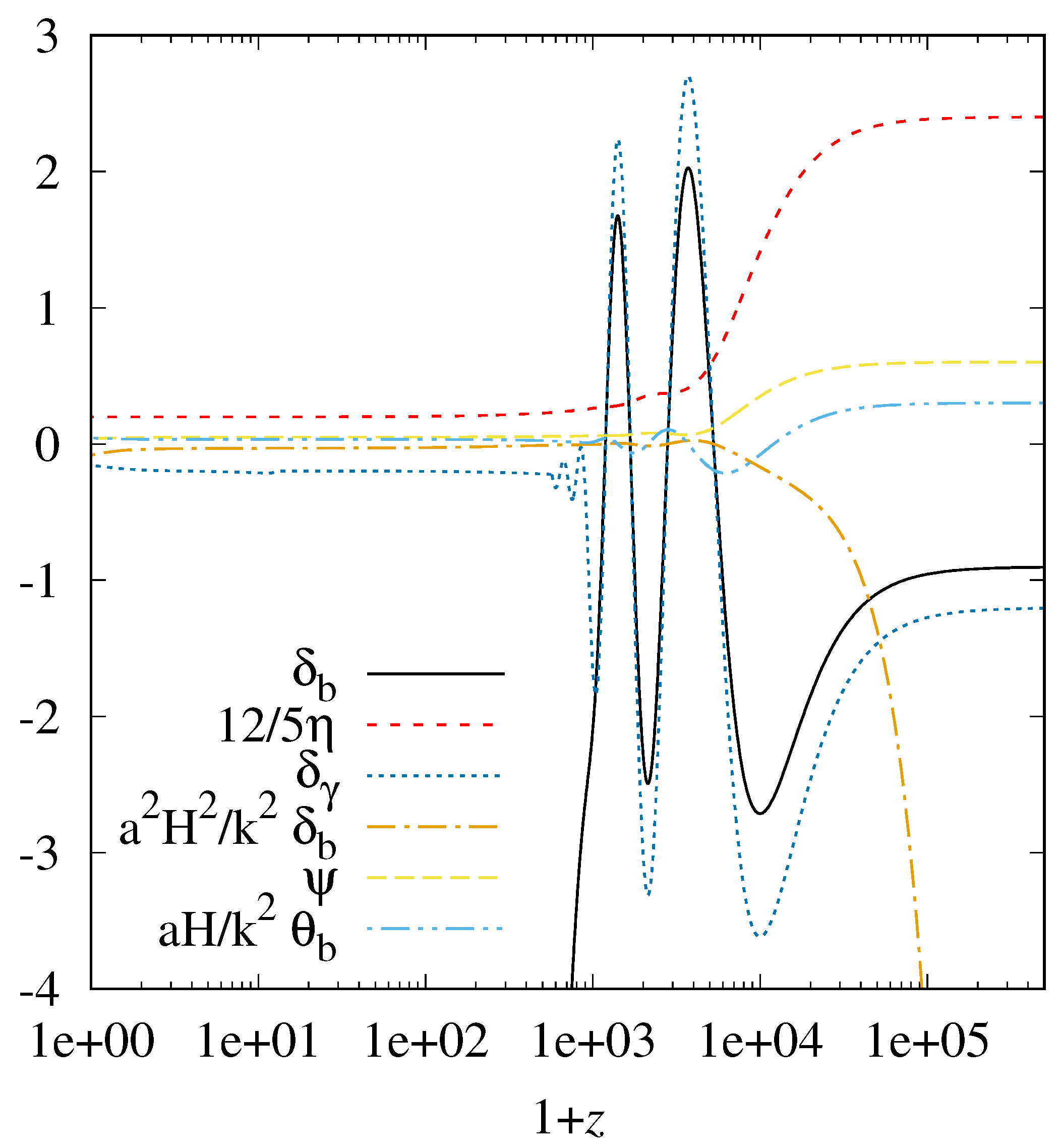
In this last equation as well, even if we consider the high k limit, we should not neglect the new terms proportional to either or . We stress once more here that the new terms we get appear only when we use the correct equations MB29–30. On using instead MB66–67, we would miss these terms all at once. In particular, as we will show in the results (compare Figure 3), we cannot neglect the term proportional to .
4. Comparison between Current Boltzmann Codes and Covariance Full Equations
In this section, we want to show explicitly that MB66–67 equations of motion for the baryons do break general covariance. This should help also the potential problem for Boltzmann solvers, which implement these equation. The results would depend on the gauge, if general covariance is broken inside the equations of motion.
Let us focus our attention on the scalar perturbations of a flat Friedmann–Lemaître–Robertson–Walker (FLRW) metric, which can be written as follows:
In the above, we have not fixed any gauge yet.
Then, on choosing the Newtonian gauge, i.e., on setting and , the equations of motion for the baryon fluid MB29–30 as given in [18] (their Equation (67)), which are also used in current Boltzmann codes, read in the Fourier space as follows:
where is the baryon density perturbation, is the scalar part of the baryon velocity perturbation defined as , is the scalar part of the photon velocity perturbation, and the term represents the momentum transfer into the photon gas. A dot here represents a derivative with respect to , the conformal time. Equations (53) and (54) are written in the Newtonian gauge, but can be rewritten in terms of the gauge invariant variables (which reduce to the corresponding perturbation variables in the Newtonian gauge when ):
as:
Since the general covariance is supposed to hold (as we are discussing general relativity in the presence of standard matter), we are now able to rewrite the previous evolution equations in any other gauge, in particular in the synchronous gauge, for which and . Then, the dynamical Equations (60) and (61) reduce to3:
where now the fields are all evaluated in the synchronous gauge. Notice that the interaction term proportional to is gauge invariant since .
Notice that the above differential equation for the velocity field, Equation (63), is different from the one written in MB66–67 (precisely Equation (66) of [18]), which is also supposed to be the baryon equation of motion written in the synchronous gauge. More precisely, the term proportional to makes the baryon velocity equation incompatible between the two gauges. To look at this same problem from another point of view, we can start by writing the dynamical baryon equations of motion in the synchronous gauge, as given in Equation (66) of [18], and then transform them to the Newtonian gauge. However, on doing so, the resulting baryon-velocity equation of motion turns out to be once again different from the one shown in Equation (54) (or Equation (67) in [18]).
Therefore, up to now, solving Boltzmann equations in the two gauges leads to solving two intrinsically different equations of motion, so that the two gauges give rise to two physically different solutions. Then, one may wonder which of the two should be considered.
First of all, it is obvious from Equation (54) that setting to vanish would make the baryon-velocity equation compatible among the two gauges; see also the results in [2] (and [28] to study its extension to second order perturbation theory).
One should now be convinced that Equations (53) and (54) break covariance, but may think this is due merely to an approximation. Let us then consider which approximation has been considered. We have already stated above that on top of considering baryons to be non-relativistic, a small scale limit has been taken, namely , but we will show it here explicitly. As we shall see later on, the correct equations of motion for the baryon fluid, in the synchronous gauge (see Footnote 3 for the redefinition of field variables), can be written as (the subscript b indicates the baryon):
whereas the non-covariant equations of motion read and . As stated in the previous section, in Boltzmann codes, is actually replaced by using the Hamiltonian constraint, which includes a term , and so, we cannot remove the term a priori, even following the Ma and Bertschinger approximation choice for baryons.
Since we only want to know the approximation done and its meaning, let us switch off the coupling with the photons, take the time derivative of , and represent this expression as where P corresponds to the rhs of Equation (65). Then, we can also write (where and time is conformal). Substituting in the rhs of such equation both and by the above given equations and replacing and (also, this latter term introduces terms proportional to ) by the Einstein equations, we can write the second order baryon equation in the form4:
On comparing this last equation with the one given in [29] for baryon sector, namely:
we see all the additional terms that have been neglected. As expected, a term proportional to has appeared, and as we shall see later in Figure 3, it cannot be neglected a priori during the radiation domination era, up to dust domination.
Nonetheless, the missing terms correspond to the realization and the definition of the approximation itself. This approximation consists of taking , (where and time is conformal) and . However, during radiation domination (valid at least for the initial conditions taken in [18] at ) at which the speed of propagation for the baryons cannot be neglected (as approximately), on considering , where , we find that k is constrained to be . Furthermore, even considering the high k limit, in the equations, we should at least keep the term proportional to .
We have another strong reason why one should not ignore the terms in that instead we have kept. Let us explain this more in detail. When we study the tight coupling approximation scheme, on using the approximated baryon equations of motion of [18], one is bound to miss some relevant terms (relevant in the sense of the point of view of [18]), e.g., (in the Newtonian gauge) and (in any gauge), which are meant, a priori, to contribute at sufficiently high k, Equation (51). Removing these terms (as they do not appear in previous Boltzmann codes) leads in general to self inconsistencies inside the regime of the validity of Ma and Bertschinger’s approximation.
As we have seen before, in Section 2, introducing back the gauge compatibility and the general covariance ends up with considering a new set of equations of motion for the baryon fluid, which will give different results from the equations found in [18]. We have also observed that making the equations of motion explicitly covariant will not make the numerical code unstable, or slow. Therefore, we do not have a clear reason why the corrections that are introduced should not be implemented in today’s Boltzmann solvers. It is true that the corrections are not large enough to change the final results beyond the error bar, but in the equations of motion, we see that these corrections (of order of ) are of a similar order as second order tight coupling approximation quantities. Therefore, implementing tight coupling approximation correctly for the aim of reaching precision cosmology should also lead to considering exact and covariant baryon equations of motion.
We point out here that there is another problem related to the gauge incompatibility of the equations of motion. In fact, since the equations of motion are not gauge compatible, we should conclude that the general covariance has been broken. In turn, this behavior leads to the fact that the equations of motion will not close in general. That is, the Bianchi identities will not hold any longer for the system of the perturbed Einstein equations. If Bianchi identities do not hold any longer, then in general, picking up a subset of equations will lead to a solution that does not solve the other remaining equations. This implies that in general, there is no solution to the full set of equations.
Finally, the new equations of motions introduced here should be considered as the basic baryon equations of motion. Therefore, any other additional physical phenomenon that has to do with baryon physics, such as reionization and higher order tight coupling approximation approximation schemes, should be considered as starting from the most basic level, i.e., from the equations of motion that we introduced in this paper.
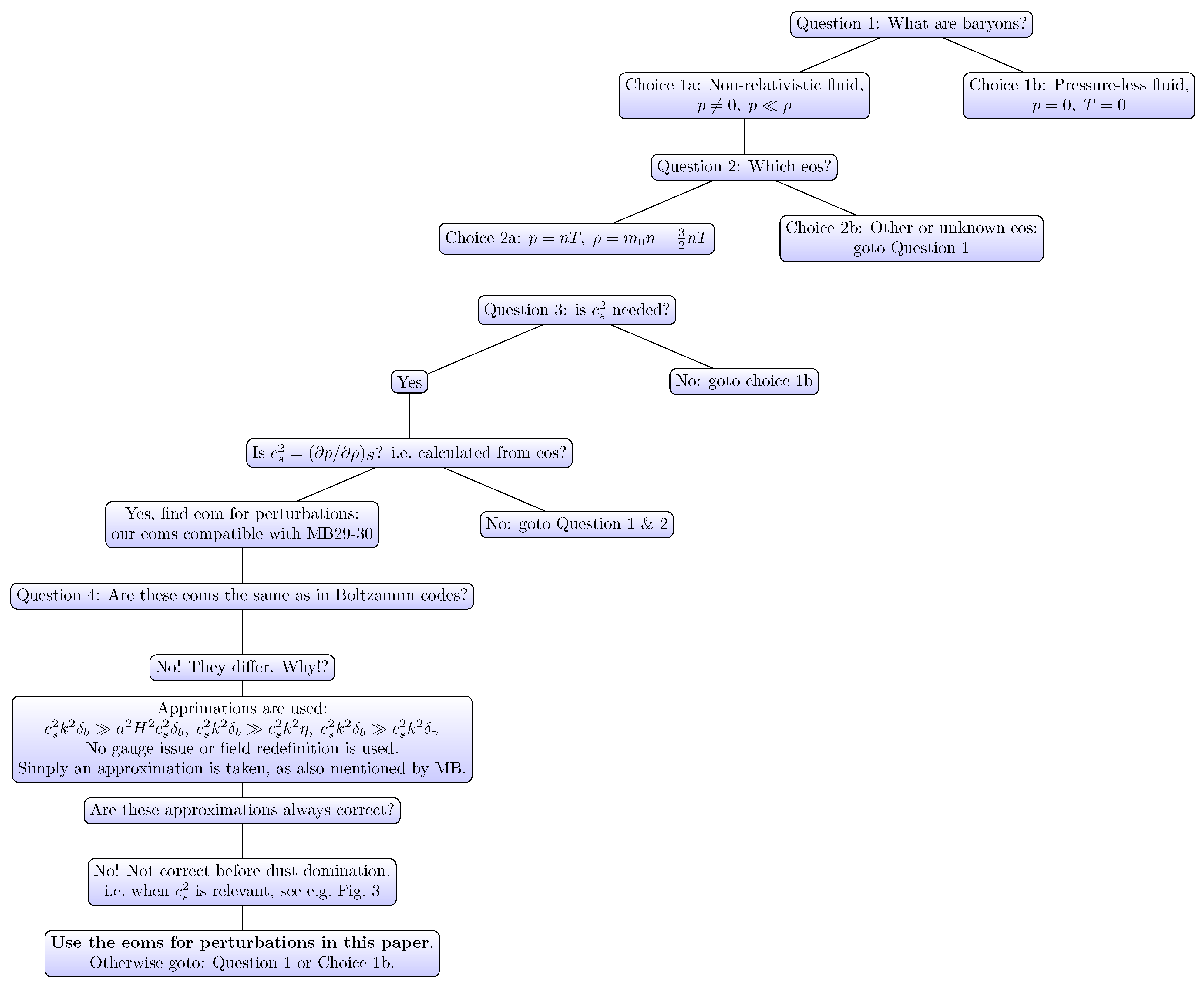
To summarize here the whole philosophy of our research path, we introduce the following tree diagram in Figure 1.
5. Code Implementation
We chose the CLASS Boltzmann solver to implement the corrected baryon and tight coupling approximation equations. We will also make our notation as close as possible to that used in [3,18]. So far, we have not fixed any gauge, but in the code, we chose the synchronous gauge for the tight coupling approximation scheme. It is straightforward to implement our approximation schemes in any other gauge.
Since we chose the synchronous gauge, . Furthermore, we will make the following field redefinitions:
CLASS has implemented five different tight coupling approximation schemes. In light of the new baryon equations, we also performed all these approximations except for the one named “second_order_CSR”. As mentioned above for the Ma & Bertschinger linear approximation scheme, we made the approximations and , for the slip parameter at first order. As for the first order CAMB, we only considered the approximation . For both first order and second order class schemes, we did not make any approximation for or .
The parameter estimation using Monte Python was carried out in a super-computer, XC-40, having 64 nodes, each node having 64 cores. In total, 4096 cores were available. We chose to run three independent series5 of 1024 chains, each chain using four cores in parallel. For each chain, we performed 13,000 steps. We ran all four tight coupling approximation schemes we implemented and found that they were all compatible with each other. On running the code, we also found that all the tight coupling approximation approximation schemes we implemented did not make the code any slower or stiffer6. In particular, the time needed by each run to terminate differed by a few minutes over approximately eight hours. As for stability, we did not have to increase precision or reduce the time step in order to solve the perturbation equations of motion. It was also noted that the acceptance rate for MCMC analysis was increased by about 0.95% for our improved code implementation with respect to the old code. This fact usually implies that the system has found a lower minimum for the . The likelihood of the covariantly corrected code was slightly improved to with respect to the old covariance breaking code for which the likelihood was .
6. Results
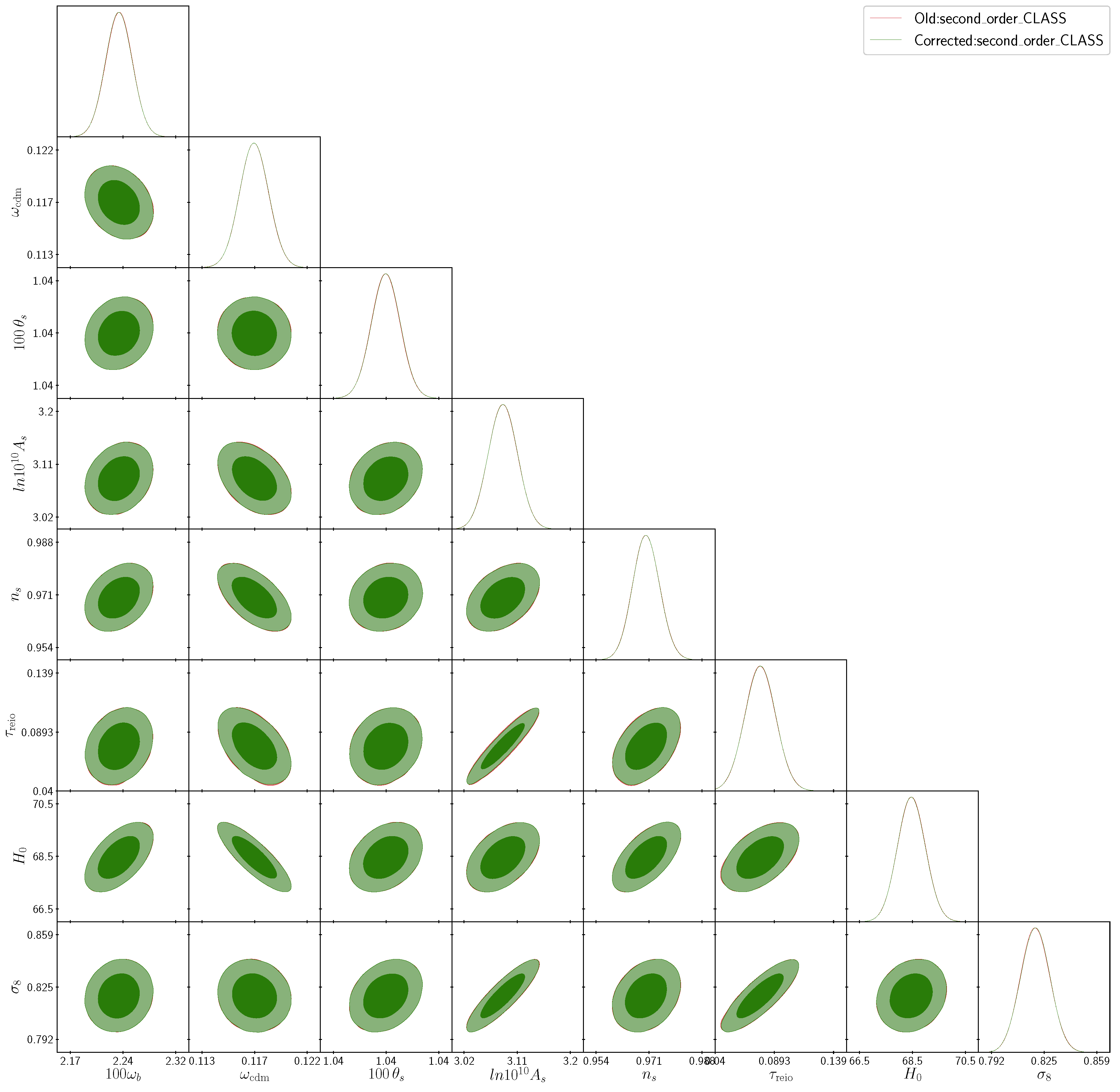
Here, we present our results of running the Monte Carlo sampler for the cosmological parameter estimation. For analysis, we used the following datasets: Planck 2015 (high l, low l, and lensing) [30], JLA [31], BAOBOSS DR12 [32], BAO SMALLZ 2014 [33,34], and Hubble Space Telescope [35]. We compared the estimation for the cosmological parameters between the old baryon equations (which were non-covariant) and the new covariant ones. We ran the Monte Python sampler for all four different tight coupling approximation schemes we implemented in CLASS, namely first_order_Ma, first_order_CAMB, first_order_CLASS, and second_order_CLASS. Below, in Table 1, we show the results for the second order tight coupling approximation scheme given by the new covariant equations of motion and the results according to old covariance breaking baryon equations of motion for the same second order tight coupling approximation scheme. Furthermore, we give combined plots of the old and the new code for the second order tight coupling approximation scheme in Figure 2. Here, we only show the numerical results for this scheme, as this is the one whose code underwent the largest number of modifications.
We found that the new results for the cosmological parameters numerically agreed with the previous results within one percent, and this fact was reassuring. Nonetheless, our corrections to the equations of motion gave a contribution that was not completely negligible, and we believe this improvement could give a useful contribution in the context of “precision cosmology” [36,37].
The amount of changes in the estimation of the parameters was similar among the different tight coupling approximation schemes we implemented. In fact, the magnitude of such changes we obtained was of the same size of the difference in the results that the original non-covariant code was giving for the different tight coupling approximation schemes. This means that in order to address the needed precision in the context of the newest (and future) cosmological probes, we should use Boltzmann solvers with the corrected covariant baryon dynamical equations.
Now that we have the results, we are in the position to justify or not the approximation taken on writing the non-covariant equations of motion for the baryons, MB66–67. Once more, in those equations and in all the ones that further make use of them, only the term was kept. As discussed before, this approximation leads to neglecting several different terms, e.g., . This approximation is justified only if we can ignore all these terms at all times at all scales. In particular, this implies that we should have or at all times. To show that this approximation fails at times before dust domination, we show in Figure 3 a plot of the perturbations , , , , (this latter one being relevant for tight coupling approximation in the Newtonian gauge), and in the high k regime, namely for at all times for the default values of the parameters. We could see once and for all that keeping only the term was not a good approximation during radiation domination and up to dust domination. Notice that this range of redshifts was exactly the era in the universe at which we should not neglect .
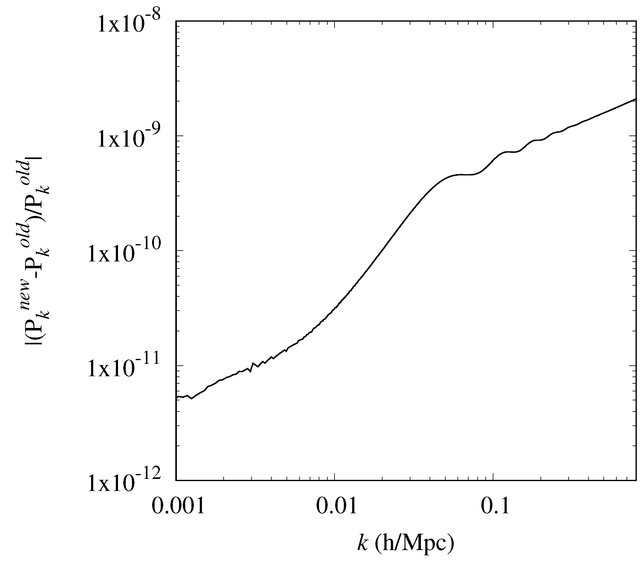
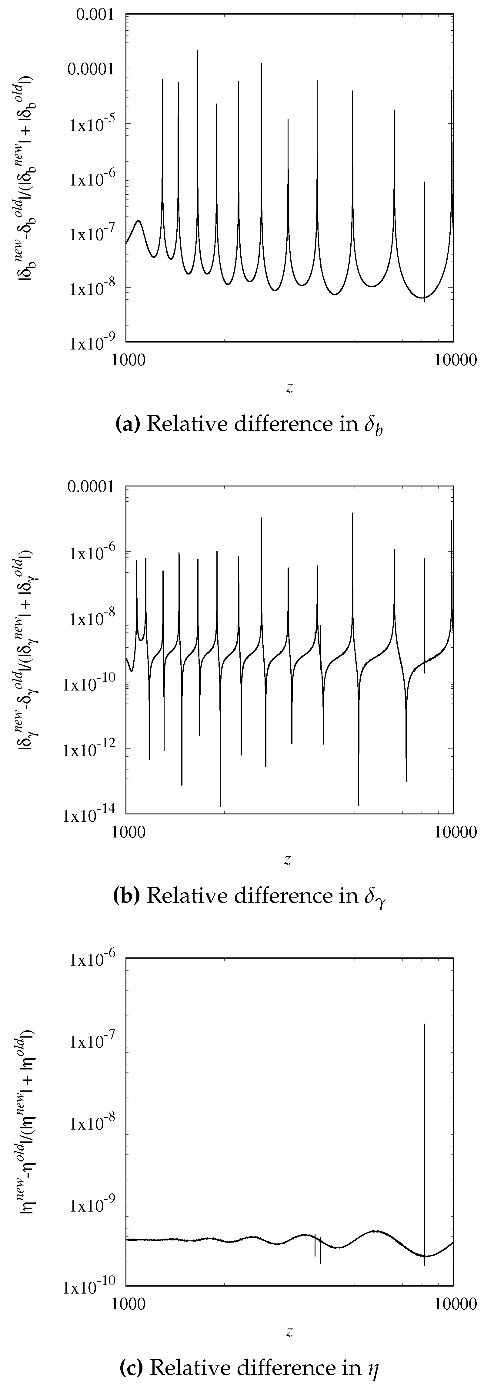
Apart from the difference in the parameter estimation (which in the end of the day, might be also correlated with finite-time parameter sampling), we also studied the relative difference in the matter power spectrum (see Figure 4) and various transfer functions (see Figure 5), at high redshifts (we chose ), for which we expected the largest corrections (because only at early times, we could consider the baryon to be non-pressureless). Indeed, we could see a difference of up to for the baryon energy-density transfer function between the two codes. Since during early times , second order tight coupling approximation was of order , then we could not neglect our corrections, as modern Boltzmann codes arrived to implement also such an approximation scheme/precision. We also give a relative difference for the perturbations , and in Figure 6. This ensured that the difference we saw was not merely numerical artifacts. In other words, we think modern Boltzmann code should implement covariant equations of motion in the baryon sector in order to be consistent with second order tight coupling approximation schemes.
Furthermore, the results presented in this work and, e.g., in Figure 3 were calculated only for CDM. If we were to study the phenomenology of some modified theory of gravity, especially for early-time modified gravity theories (which in general are implemented as not affecting directly the matter equations of motion that come from conservation of the stress-energy tensor), we could expect non-trivial behavior from the metric field perturbations (in the synchronous gauge) or (in the Newtonian gauge), which could change the results of Figure 3. A priori, we would not be sure that the gravitational perturbation field could be really neglected. This may result in missing relevant information in studying the cosmology of modified theories of gravity. Keeping equations that obey general covariance ensured we did not miss any information within the theory.
7. Conclusions
In this paper, we pointed out that there were at least three conceptual issues in the implementation of the seminal work by Ma and Bertschinger [18] in existing Boltzmann codes due to some missing terms. Those missing terms were numerically small and usually neglected, but led to the following conceptual issues: (i) the baryon equations were not gauge compatible; (ii) these equations violated the Bianchi identity; (iii) the origin of the term with was not clear. To address all these issues, we imposed the free Lagrangian of baryons to be described by the covariant action of a non-relativistic ideal gas. We found that this model for the baryon fluid, which described a non-relativistic system of particles with a non-zero temperature and , led to covariant equations of motion for the perturbations, which did not violate the Bianchi identities. We also derived the same equations from the conservation of the stress-energy tensor, without relying on the Lagrangian.
Since the new covariant equations of motion for baryons represent one of the main results of our paper, we will rewrite them here both in the synchronous and Newtonian gauge, in the notation of [18], as follows.
Synchronous gauge:
Conformal Newtonian gauge:
where the new contributions (with respect to [18]) come from Lines (72b), (73b), (74b), and (75b).
Furthermore, with our new equations, we can keep terms that were before completely omitted in the previous equations of motion. For example on taking the time derivative of Equation (73), which can be written schematically as , we find . On replacing into this new equation the value of with its own equation of motion, Equation (72), together with the Einstein equations (to remove the fields and ), we get the standard term , but also other terms, e.g., one proportional to ( being the curvature perturbation in the synchronous gauge), which cannot be neglected a priori, but was absent in previous treatments of baryon physics. In this same equation, also other terms have been in the past neglected, e.g., terms proportional to , and from Equation (72b), a term proportional to . Therefore, the approximations made in the past correspond to setting , , and . However, during radiation domination (valid at least for the initial conditions taken in [18] at ), on approximating , where , we find that k is constrained to be . Furthermore, (at any time and scale), and . However, several authors, e.g., [18], considered a range for k given by , so that inside this set, the previous approximations in general failed for large redshifts. One may wonder then why our numerical results were still similar to the previous ones. The reason was that was anyhow a small quantity, which gave only a small correction to the baryon-dust fluid (i.e., a fluid with identically equal to zero). Nonetheless, we claim that only our approximation can be trusted, as the contributions we introduced restored general covariance and were the only terms consistent with cosmological linear perturbation theory. We believe that the percent level correction for the parameter estimation that we found is expected to be important for future surveys [36,37].
With the covariant action so introduced, we claim we fixed all three issues of [18] stated above. In fact, the new equations of motion for the baryon fluid possessed additional terms of order , which made the system of differential equations gauge compatible, hence obeying the general covariance.
In order to understand the cosmological evolution at all relevant redshifts, we need to study the solution of the equations of motion before recombination. In this regime, photons and baryons are tightly coupled, leading in general to a stiff regime during which it is difficult to solve the equations of motion numerically. In order to overcome this problem, we adapted several approximate schemes, already introduced in the past, to our new dynamical equations of motion. We then found the solutions of the equations of motion for the perturbations up to the second order in the tight coupling approximation using the new corrected baryon dynamics. In fact, we implemented four different tight coupling approximation schemes without choosing any gauge, so that our code could then be immediately used in any gauge for modern Boltzmann solvers.
We therefore used a Monte Carlo sampler in order to re-estimate the values of the cosmological parameters, after having incorporated our covariant corrections into the baryon dynamical equations of motion. We found that there were some parameters, e.g., , whose best fit values deviated from the previous code analysis by one percent. Moreover, we did not a priori know whether the deviation remained as small as one percent in other models and various modified gravity theories. In the age of precision cosmology, we therefore believe that these changes are to be considered. On top of that, we found that both the covariantly corrected baryon equations of motion and the baryon-photon fluid tight coupling approximation schemes did not make the code (implemented in CLASS) slower or stiffer than the previous code. Hence, we did not find any reason why the modifications presented in this paper to the code should not be included permanently into modern Boltzmann codes, so as to confront any gravity theory with the present and future observations in the era of precision cosmology.
Author Contributions
All authors have equally contributed to the the whole paper. All authors have read and agreed to the published version of the manuscript.
Funding
The work of S.M. was supported by Japan Society for the Promotion of Science (JSPS) Grants-in-Aid for Scientific Research (KAKENHI) No. 17H02890, No. 17H06359, and by the World Premier International Research Center Initiative (WPI), MEXT, Japan. M.C.P. acknowledges the support from the Japanese Government (MEXT) scholarship for Research Student.
Acknowledgments
We thank Julien Lesgourgues and Antony Lewis for suggestions and comments. The numerical computation in this work was carried out at the Yukawa Institute Computer Facility.
Conflicts of Interest
The authors declare no conflict of interest.
Appendix A. Speed of Propagation of Matter Fields in the Presence of Several Fluids
In the following, we want to consider the case of N different fluids. For simplicity, we will consider the case of several perfect fluids. For each of the fluids, we need to give equations of state, namely:
which together with the first principle of thermodynamics, namely:
where , are enough to completely specify the thermodynamics of the ith fluid, provided the integrability condition holds, namely:
For any of the fluids, we have then automatically the speed of propagation:
So far, the discussion holds in any environment, in particular in cosmology. In the latter, the equations of state hold at any order in perturbation theory, so that for relativistic degrees of freedom , not only at the level of the background, but at any order in perturbation theory. In particular, at first order of perturbation theory, we have:
where the overline tells us we need to consider the quantities evaluated at the background level. Therefore, for fluids, whether or not in the presence of other fluids, the expression of the speed of propagation does not change. In particular, a dust fluid (for which ) will have , whereas for a radiation fluid . The thermodynamical description of the fluid, well described in [27], is powerful in particular for non-barotropic fluids, such as ideal gas, for which p is not only a function of . The speed of propagation in any fluid does correspond to the adiabatic speed. It should be noticed that this holds for fluids. In the case of a general action for a scalar field, e.g., quintessence, this formalism cannot be applied, and the speed of propagation needs to be studied for the particular action at hand.
We want to add here a discussion on the equations of state for baryons in particular. One can choose several (but all equivalent to each other) equations of state for the baryon fluid. In particular, one can choose , which is absolutely fine, because a thermodynamical equation of state can be written in terms of any two thermodynamical degrees of freedom, for example or as discussed, e.g., on p. 564 of [27]. Then, it is obvious that the pressure perturbation should be of the form:
Equivalently, we can consider as discussed in this paper . These two descriptions are actually completely equivalent. In fact, since the thermodynamical degrees of freedom are two, we can also write , and hence, . Then, one can show that:
for adiabaticity. This adiabaticity condition is also correctly considered in Ma and Bertschinger, being stated before their Equation (96).
Appendix B. Ideal Gas
One of the main points of our paper is to show indeed that the equations of motion used in Boltzmann codes for the baryon fluid do not satisfy energy-momentum conservation. Therefore, we find it appropriate to enucleate the problem from another point of view. Each equation of motion by itself defines automatically the system under study. Therefore, one could try to understand what kind of matter is described by the equations of motion for baryons used in Boltzmann codes.
To reach this goal, it is sufficient to consider these equations of motion (MB66–67) and set to zero the interaction with the photon gas. This should then define the self-gravitating physical system under consideration. Then, the covariance breaking equations of motion in the Newtonian gauge read as:
The problems is that in this limit, the fluid does not reduce either to a dust fluid or to any other perfect fluid equations of motions. The free equations describe an unknown system, which cannot be described in terms of a perfect fluid in general relativity. That is the reason why these same equations break general covariance. In this same case, we should also expect that these equations cannot come from a Lagrangian, and therefore, they cannot be found by any conservation law, i.e., they cannot come from considering .
Therefore, in order to reintroduce general covariance, we impose that the free Lagrangian for the baryon reduces to the Lagrangian of an ideal gas, because we are interested in a non-zero sound speed of propagation, i.e., . In fact, a perfect fluid for baryons may be modeled in two possible ways, with or without temperature. The model without temperature is described by a dust fluid. However, this model would lead to , and this is not the model for which we are looking. Let us consider then the case of a baryon fluid with a tiny, but non-zero temperature, as only in this case, the baryon fluid will possess . The model for baryons considered here consists of an ideal gas, whose fluid particles are considered to be non-relativistic. To this fluid gas, a collision term with photons will be then added, as we do in the case of a dust-like baryon-gas without temperature.
A monoatomic ideal gas is defined by the following two equations of state:
where and T are the pressure, number density, energy density, and temperature of the fluid, respectively. Furthermore, is a constant and represents the mass of the fluid particle. Since the fluid is assumed to be non-relativistic, these equations of state hold only for . Indeed, as shown in Section 2.1, we have performed an expansion of the equations of motion for the baryon sector with respect to this small parameter.
The first law of thermodynamics for a general perfect fluid (see, e.g., [27]) can be written as:
where the enthalpy per particle is defined as:
and s represents the entropy per particle. Therefore, on considering , we find:
On combining the two equations of state (A11), it is easy to show that:
which shows that an ideal gas does not represent a fluid with a barotropic equation of state because ; instead, we have . Furthermore, this equation shows that for an ideal gas , so that at the zeroth order in , this fluid can be well approximated by a dust fluid. However, whenever in the history of the universe, on cosmological scales, the speed of propagation for the baryon fluid cannot be neglected, then we have7:
confirming Equation (68) in [18] at the first approximation. Hereafter, by an overdot, we represent the derivative with respect to the conformal time .
In particular, this shows that we cannot in general neglect the pressure of such a fluid, and we have:
In the presence of a collision term with photons, there is an exchange of entropy with the photon fluid, which when combined with the first law of thermodynamics gives:
as shown in [18].
Appendix C. Tight Coupling Approximation: Detailed Calculation
Here, we discuss the tight coupling approximation up to the second order with corrected equations of baryons.
We have the following set of equations for the photon fluid, without fixing any gauge [18]8:
where , is higher multipoles of the photon Boltzmann hierarchical equations, and is multipoles of Boltzmann hierarchical equations for the difference in the photon linear polarization components [2,18].
We can rewrite the two equations for the speed of photons and baryons, given respectively by (A21) and (33), as:
where9:
Then, adding both of these equations, we obtain:
where The above equation determines the evolution of , which is often referred to as the slip parameter. Equation (A28) involves the shear of photons. The shear Equation (A22) for the photon can be rewritten as,
We can consider linear combinations of Equations (A25) and (A26) in order to eliminate , so that we find:
From the above equation, we obtain the equation for as:
All these equations are exact. In what follows, we will mainly use Equations (A27)–(A29), and (A33) in order to find approximate solutions for and .
Appendix C.1. Terms in G
In the equation of motion for the shear, Equation (A24), there appear terms in and . Let us first see the perturbative solution of these two terms. Consider the equation for with ,
with the assumption, to be confirmed later on, that and and that is even more suppressed. In this case, let us look for solutions of the kind:
Then, we find:
where we have assumed that , which is valid, as long as the tight coupling approximation is meaningful. This last equation leads to the lowest order to:
Then:
or, to the lowest order now:
and:
so that:
and:
A similar argument leads to:
Now, we need to verify that indeed and . In fact, we have:
so that on looking for solutions of the kind and we find:
so that, at the lowest order, we find:
or:
Here, we assume for the moment that . We will check later on that this assumption is consistent. Then, at the next order:
or:
which leads to:
and to:
For general , we have:
and since there are no source terms, we will assume that each term is suppressed by with respect to the term, that is:
so that we find:
or:
which leads, at leading order, to:
or:
so that we find
Since we obtain the same equations of motion for the terms for , then we also have:
Appendix C.2. Shear Solution
Now, we need to look for an approximate solution for the shear. Using the solutions for and , we can rewrite Equation (A22) as:
which leads to:
and:
Now, let us assume that we have a solution of the form:
then we obtain:
which at the lowest order leads to:
so that, at the next order, we have:
or:
Hence, we find the approximate solution as:
This approximate solution agrees with the one found in [3].
Appendix C.3. Slip Equation
From now on, because we will make use of the new equations of motion for the baryon fluid, our results will start differing from the ones given in [3]. To find an approximate solution for the slip parameter, up to the second order in , let us start with Equation (A28):
and let us search for a solution for . Then, we have, up to the second order:
At the lowest order, we find:
or:
The solution is then found as:
In the following, we will rewrite the above solution for the slip parameter in such a way that we can easily implement them in the new CLASS code.
Appendix C.4. First Order Contribution
We first manipulate the first order solutions as follows:
In this equation, we replace the quantity (which appears inside ) with its solution for Equation (A26), , , and the quantity with Equation (A81). It should be noticed that Equation (A26) comes in the form:
Therefore, when we replace , and we will end up with an overall coefficient of that partly depends on and partly on another coefficient that, in turn, depends on the free function . Then, we choose so that the result looks as close as possible to the result given in [3] (Equation (2.19)), namely:
Appendix C.5. Second Order Contribution
As we already know, at the second order, we find:
where:
Therefore, we can substitute all the terms inside Equation (A88). This will lead to substituting , , , , , , .
We then obtain a quite complicated expression that corresponds to the needed answer for the slip parameter valid up to the second order in . However, once more, we try to write it as close as possible to the expression written in [3]. Then, we write:
In this last line, we should think that the quantities are given explicitly, whereas is left as it is. Then, we still add new contributions:
where the functions are supposed to be of order , and in the very last line, the equality holds up to the second order in . Therefore, we can rewrite:
where:
Furthermore, we can easily find the decomposition of:
into the linear and quadratic contributions.
Let us then focus on . This term will contain terms of the kind , , , and we replace them respectively by , , as their difference appears at the cubic order. Once these terms are replaced, we can, in turn, replace the expressions of and by using the zeroth order approximation found by using Equation (A33), which can be written as:
This substitution is allowed because it is performed inside the quadratic term . It can be checked that now in , there is no more explicit term containing or any of its derivatives. Furthermore, there is no more explicit dependence on . In the end, after all these substitutions, we have . However, in the linear contribution, we have a non-zero contribution from the term . For such a term, we can replace the exact solution coming from solving Equation (A26), as in:
This term will modify the coefficient of the term . Then, we can choose the variables so that the linear result looks as similar as possible to the one written in Equation (2.20) of [3]. Namely, we choose:
so that in this case, the slip equation reduces to:
so that the linear term (excluding the terms explicitly dependent on ) exactly coincides with the quantity . We can finally add and subtract a quadratic order term to end up with:
where:
Here, the expressions for have been replaced in . Now, we are only left with the implementation of these results in the CLASS code.
References
- Kodama, H.; Sasaki, M. Cosmological Perturbation Theory. Prog. Theor. Phys. Suppl. 1984, 78, 1–166. [Google Scholar] [CrossRef]
- Dodelson, S. Modern Cosmology; Academic Press: Amsterdam, The Netherlands, 2003. [Google Scholar]
- Blas, D.; Lesgourgues, J.; Tram, T. The Cosmic Linear Anisotropy Solving System (CLASS) II: Approximation schemes. J. Cosmol. Astropart. Phys. 2011, 2011, 034. [Google Scholar] [CrossRef] [Green Version]
- Lewis, A.; Challinor, A.; Lasenby, A. Efficient computation of CMB anisotropies in closed FRW models. Astrophys. J. 2000, 538, 473–476. [Google Scholar] [CrossRef] [Green Version]
- Doran, M. CMBEASY: An object oriented code for the cosmic microwave background. J. Cosmol. Astropart. Phys. 2005, 2005, 011. [Google Scholar] [CrossRef]
- Seljak, U.; Zaldarriaga, M. A Line of sight integration approach to cosmic microwave background anisotropies. Astrophys. J. 1996, 469, 437–444. [Google Scholar] [CrossRef] [Green Version]
- Laureijs, R.; Amiaux, J.; Arduini, S.; Auguères, J.-L.; Brinchmann, J.; Cole, R.; Cropper, M.; Dabin, C.; Duvet, L.; Ealet, A.; et al. Euclid Definition Study Report. Available online: https://arxiv.org/abs/1110.3193 (accessed on 30 December 2019).
- Aghamousa, A. [DESI Collaboration]. The DESI Experiment Part I: Science, Targeting, and Survey Design. Available online: https://arxiv.org/abs/1611.00036 (accessed on 30 December 2019).
- Zhan, H.; Tyson, J.A. Cosmology with the Large Synoptic Survey Telescope: An Overview. Rept. Prog. Phys. 2018, 81, 066901. [Google Scholar] [CrossRef] [Green Version]
- Lifshitz, E. Republication of: On the gravitational stability of the expanding universe. Gen. Relativ. Gravit. 2017, 49, 18. [Google Scholar] [CrossRef]
- Bardeen, J.M. Gauge Invariant Cosmological Perturbations. Phys. Rev. 1980, D22, 1882–1905. [Google Scholar] [CrossRef]
- Sugiyama, N.; Gouda, N. Perturbations of the Cosmic Microwave Background Radiation and Structure Formations. Prog. Theor. Phys. 1992, 88, 803–844. [Google Scholar] [CrossRef]
- Sugiyama, N. Cosmic background anistropies in CDM cosmology. Astrophys. J. Suppl. 1995, 100, 281. [Google Scholar] [CrossRef]
- White, M.J.; Scott, D. Why not consider closed universes? Astrophys. J. 1996, 459, 415. [Google Scholar] [CrossRef] [Green Version]
- Hu, W.; White, M.J. CMB anisotropies: Total angular momentum method. Phys. Rev. 1997, D56, 596–615. [Google Scholar] [CrossRef] [Green Version]
- Hu, W.; Seljak, U.; White, M.J.; Zaldarriaga, M. A complete treatment of CMB anisotropies in a FRW universe. Phys. Rev. 1998, D57, 3290–3301. [Google Scholar] [CrossRef] [Green Version]
- Bertschinger, E. COSMICS: Cosmological Initial Conditions and Microwave Anisotropy Codes. Available online: https://arxiv.org/abs/astro-ph/9506070 (accessed on 30 December 2019).
- Ma, C.-P.; Bertschinger, E. Cosmological perturbation theory in the synchronous and conformal Newtonian gauges. Astrophys. J. 1995, 455, 7–25. [Google Scholar] [CrossRef] [Green Version]
- Peebles, P.J.E.; Yu, J.T. Primeval adiabatic perturbation in an expanding universe. Astrophys. J. 1970, 162, 815–836. [Google Scholar] [CrossRef]
- Cyr-Racine, F.Y.; Sigurdson, K. Photons and Baryons before Atoms: Improving the Tight-Coupling Approximation. Phys. Rev. 2011, D83, 103521. [Google Scholar] [CrossRef] [Green Version]
- Pitrou, C. The tight-coupling approximation for baryon acoustic oscillations. Phys. Lett. 2011, B698, 1–5. [Google Scholar] [CrossRef] [Green Version]
- Schutz, B.F.; Sorkin, R. Variational aspects of relativistic field theories, with application to perfect fluids. Annals Phys. 1977, 107, 1–43. [Google Scholar] [CrossRef] [Green Version]
- Brown, J.D. Action functionals for relativistic perfect fluids. Class. Quantum Gravity 1993, 10, 1579–1606. [Google Scholar] [CrossRef] [Green Version]
- De Felice, A.; Gerard, J.-M.; Suyama, T. Cosmological perturbations of a perfect fluid and noncommutative variables. Phys. Rev. 2010, D81, 063527. [Google Scholar] [CrossRef] [Green Version]
- Audren, B.; Lesgourgues, J.; Benabed, K.; Prunet, S. Conservative Constraints on Early Cosmology: An illustration of the Monte Python cosmological parameter inference code. J. Cosmol. Astropart. Phys. 2013, 02, 001. [Google Scholar] [CrossRef] [Green Version]
- Brinckmann, T.; Lesgourgues, J. MontePython 3: Boosted MCMC sampler and other features. Phys. Dark Univ. 2019, 24, 100260. [Google Scholar] [CrossRef] [Green Version]
- Misner, C.W.; Thorne, K.S.; Wheeler, J.A. Gravitation; Princeton University Press: Princeton, NJ, USA, 2017. [Google Scholar]
- Bartolo, N.; Matarrese, S.; Riotto, A. Cosmic Microwave Background Anisotropies up to Second Order. Available online: https://arxiv.org/abs/astro-ph/0703496 (accessed on 30 December 2019).
- Lewis, A. Linear effects of perturbed recombination. Phys. Rev. 2007, D76, 063001. [Google Scholar] [CrossRef] [Green Version]
- Adam, R. [Planck Collaboration]. Planck 2015 results. I. Overview of products and scientific results. Astron. Astrophys. 2016, 594, A1. [Google Scholar]
- Betoule, M.; Kessler, R.; Guy, J.; Mosher, J.; Hardin, D.; Biswas, R.; Astier, P.; El-Hage, P.; Konig, M.; Kuhlmann, S.; et al. Improved cosmological constraints from a joint analysis of the SDSS-II and SNLS supernova samples. Astron. Astrophys. 2014, 568, A22. [Google Scholar] [CrossRef]
- Alam, S.; Ata, M.; Bailey, S.; Beutler, F.; Bizyaev, D.; Blazek, J.A.; Bolton, A.S.; Brownstein, J.R.; Burden, A.; Chuang, C.-H.; et al. The clustering of galaxies in the completed SDSS-III Baryon Oscillation Spectroscopic Survey: Cosmological analysis of the DR12 galaxy sample. Mon. Not. R. Astron. Soc. 2017, 470, 2617–2652. [Google Scholar] [CrossRef] [Green Version]
- Beutler, F.; Blake, C.; Colless, M.; Jones, D.H.; Staveley-Smith, L.; Campbell, L.; Parker, Q.; Saunders, W.; Watson, F. The 6dF Galaxy Survey: Baryon acoustic oscillations and the local Hubble constant. Mon. Not. R. Astron. Soc. 2011, 416, 3017–3032. [Google Scholar] [CrossRef]
- Ross, A.J.; Samushia, L.; Howlett, C.; Percival, W.J.; Burden, A.; Manera, M. The clustering of the SDSS DR7 main Galaxy sample—I A 4 per cent distance measure at z = 0.15. Mon. Not. R. Astron. Soc. 2015, 449, 835–847. [Google Scholar] [CrossRef] [Green Version]
- Riess, A.G.; Macri, L.M.; Hoffmann, S.L.; Scolnic, D.; Casertano, S.; Filippenko, A.V.; Tucker, B.T.; Reid, M.J.; Jones, D.O.; Silverman, J.M.; et al. A 2.4% Determination of the Local Value of the Hubble Constant. Astrophys. J. 2016, 826, 56. [Google Scholar] [CrossRef]
- Ade, P.; Aguirre, J.; Ahmed, A.; Aiola, S.; Ali, A.; Alonso, D.; Alvarez, M.A.; Arnold, K.; Ashton, P.; Austermann, J.; et al. The Simons Observatory: Science goals and forecasts. J. Cosmol. Astropart. Phys. 2019, 02, 056. [Google Scholar] [CrossRef]
- Lazear, J.; Ade, P.A.R.; Benford, D.; Bennett, C.L.; Chuss, D.T.; Dotson, J.L.; Eimer, J.R.; Fixsen, D.J.; Halpern, M.; Hilton, G.; et al. The primordial inflation polarization explorer (piper). In Proceedings of the Millimeter, Submillimeter, and Far-Infrared Detectors and Instrumentation for Astronomy VII, Montréal, QC, Canada, 22–27 June 2014. [Google Scholar]
| 1. | We provide our new code in the link http://www2.yukawa.kyoto-u.ac.jp/~antonio.defelice/new_baryon.zip. |
| 2. | Here, we have used the conventions of Ma and Bertschinger for the metric perturbation fields , h. |
| 3. | The relation between fields defined in this paper and definitions used in CLASS are and . For the synchronous gauge, we add the gauge choice , , which is actually incomplete. For a complete gauge fixing, we need to choose also the following two initial conditions at the time : , , where represents the field for the cold dark matter fluid and is the photon density perturbation. For the Newtonian gauge, the authors in [18] used the following field redefinition, , , together with the complete gauge fixing, , . |
| 4. | The extra terms in is due to the fact that Equations (64) and (65) have terms that are not neglected a priori. On using Einstein equations in the synchronous gauge, one gets these extra terms; especially, the term , which can never be neglected since in the relevant redshift range, as we show in Figure 3. |
| 5. | One for each author. |
| 6. | The code can be found at http://www2.yukawa.kyoto-u.ac.jp/~antonio.defelice/new_baryon.zip. |
| 7. | It should be noted that for a general perfect fluid, the notion of the sound speed is purely thermodynamical, so that once the equations of state are imposed, its expression is independent of the background. For an ideal gas, we find . Furthermore, since p can be written in terms of two other thermodynamical variables, we have that at linear order , which can be rewritten as . In particular, we find that, in general, . |
| 8. | In the case of non-flat 3D slices, the equations of motion need to be changed. For example, in Equation (A21), the shear field gets an extra factor, , where, following the CLASS code notation, . |
| 9. | We have neglected the contribution from the baryon pressure from the term , because the correction term, typically of order of , will affect the tight coupling approximation only at higher orders (e.g., the cubic order). |
| 10. | If the background spatial curvature is present, then, as already mentioned in Footnote 8, we need to replace . |
Figure 1.
Tree diagram that describes the logic followed in this paper to address the issue of non-conservation of energy-momentum in the equations of motion MB66–67 for baryons in existing Boltzmann codes.
Figure 1.
Tree diagram that describes the logic followed in this paper to address the issue of non-conservation of energy-momentum in the equations of motion MB66–67 for baryons in existing Boltzmann codes.

Figure 2.
Combined results given by the old, original CLASS code with covariance breaking equations of motion for the baryon and the new code with covariant equations of motion for the baryon fluid. The percent level differences shown in Table 1 are invisible in this figure, but will be important for future surveys.

Figure 3.
Evolution of perturbations out of which we can test the motivation of our study in the high k regime (fixing ) at all times for the default values of the parameters. During radiation domination (when should not be neglected) and up to , typically dominates over , so that , and this term cannot be neglected. Instead, dominates over up to , so that in this range of redshift . Therefore, such a term cannot be neglected in tight coupling approximation schemes. Finally, even for this high k mode, the subhorizon approximation breaks down during radiation domination, as it is clear that for , we have . Since cannot be neglected in this redshift range, also this term should be included in the equations of motion for the perturbations. All these new terms are terms that are imposed by conservation of the stress-energy tensor.

Figure 4.
Relative difference in the matter power spectrum at . We fixed the same background parameters for both codes, so that the error only depends on the difference in the equations of motion for the baryon-photon sector.
Figure 4.
Relative difference in the matter power spectrum at . We fixed the same background parameters for both codes, so that the error only depends on the difference in the equations of motion for the baryon-photon sector.

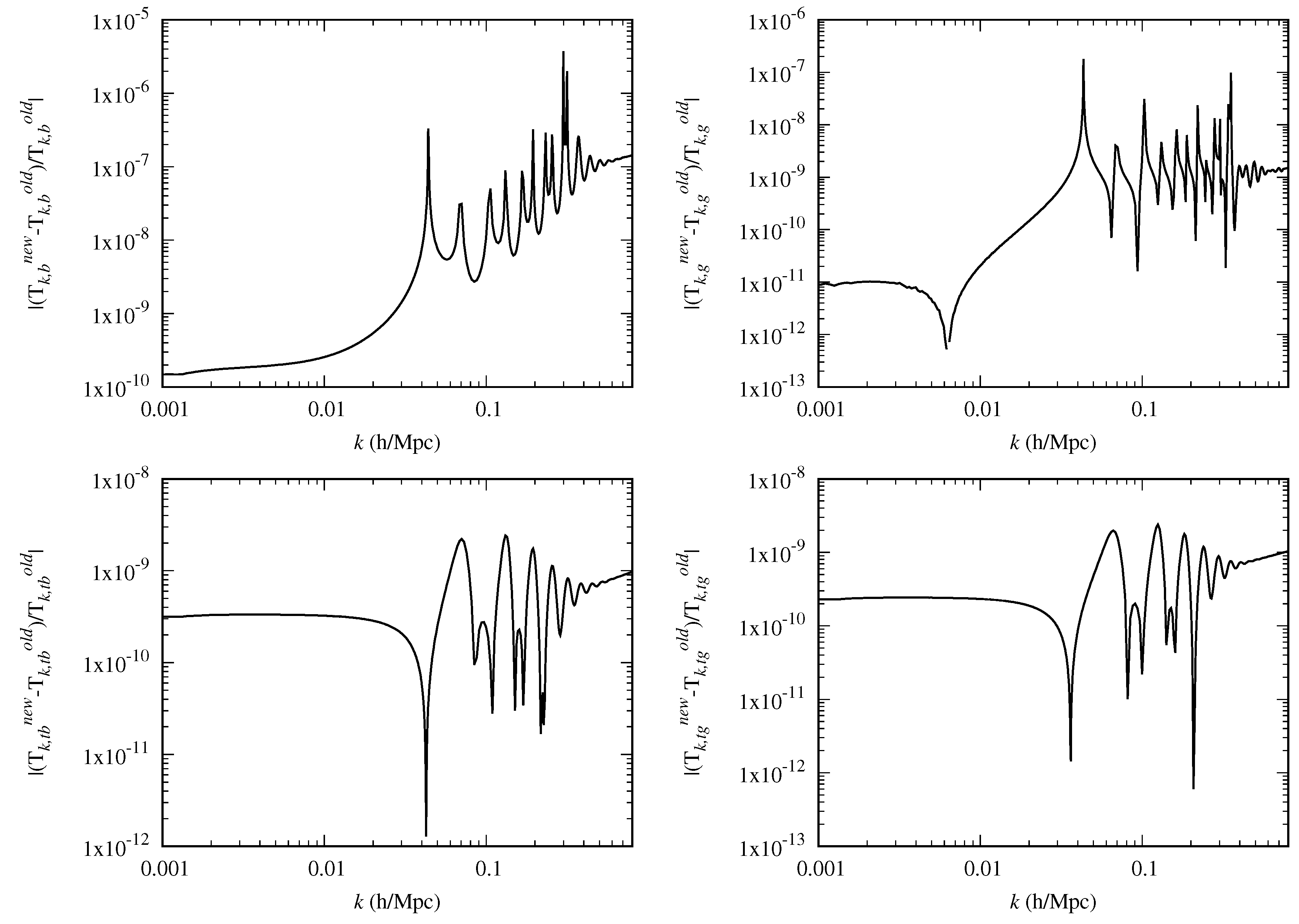
Figure 5.
Relative difference in the transfer function for , , , and at . The y-axis gives the relative error between covariant results and non-covariant results. The error increases at higher values of k and reaches values of order for .
Figure 5.
Relative difference in the transfer function for , , , and at . The y-axis gives the relative error between covariant results and non-covariant results. The error increases at higher values of k and reaches values of order for .

Figure 6.
Relative difference in various perturbation fields. The spikes are due to oscillations crossing zero. In order to obtain these figures, we increased the precision of CLASS (simply by setting a lower tolerance for integrating the equations of motion). Furthermore, we had to interpolate the numerical results in order to be able to evaluate and compare the fields at the same point.


Table 1.
Best fit values of cosmological parameters given by MCMC analysis: old vs. new. The upper and lower limits are at the 95% confidence level.
Table 1.
Best fit values of cosmological parameters given by MCMC analysis: old vs. new. The upper and lower limits are at the 95% confidence level.
| Parameters | Best Fit: New (Old) | Relative % Change in the Best Fit |
|---|---|---|
© 2019 by the authors. Licensee MDPI, Basel, Switzerland. This article is an open access article distributed under the terms and conditions of the Creative Commons Attribution (CC BY) license (http://creativecommons.org/licenses/by/4.0/).
Share and Cite
MDPI and ACS Style
C. Pookkillath, M.; De Felice, A.; Mukohyama, S. Baryon Physics and Tight Coupling Approximation in Boltzmann Codes. Universe 2020, 6, 6. https://doi.org/10.3390/universe6010006
AMA Style
C. Pookkillath M, De Felice A, Mukohyama S. Baryon Physics and Tight Coupling Approximation in Boltzmann Codes. Universe. 2020; 6(1):6. https://doi.org/10.3390/universe6010006
Chicago/Turabian StyleC. Pookkillath, Masroor, Antonio De Felice, and Shinji Mukohyama. 2020. "Baryon Physics and Tight Coupling Approximation in Boltzmann Codes" Universe 6, no. 1: 6. https://doi.org/10.3390/universe6010006
Note that from the first issue of 2016, this journal uses article numbers instead of page numbers. See further details here.