Influence of Microfield Directionality on Line Shapes

Abstract

In the framework of the Spectral Line Shapes in Plasmas Code Comparison Workshop (SLSP), large discrepancies appeared between the different approaches to account for ion motion effects in spectral line shape calculations. For a better understanding of these effects, in the second edition of the SLSP in August, 2013, two cases were dedicated to the study of the ionic field directionality on line shapes. In this paper, the effects of the direction and magnitude fluctuations are separately analyzed. The effects of two variants of electric field models, (i) a pure rotating field with constant magnitude and (ii) a time-dependent magnitude field in a given direction, together with the effects of the time-dependent ionic field on shapes of the He II Lyman-α and -β lines for different densities and temperatures, are discussed.

1. Introduction

The effect of ionic field fluctuations on spectral line shapes of hydrogen and hydrogen-like emitters has been studied for a long time by different groups. In the 1970s, the observed deviations between experiments and theories were attributed to ion motion. At the same time, the first attempts to include ion motion effects in theories appeared [1,2,3,4,5], and the experimental proof on hydrogen had been obtained nearly concomitantly by Wiese and co-workers [6,7]. The first N-body molecular dynamics simulations appeared in the the late 1970s [8].

Nowadays, large differences still appear between the various approaches to take into account the effect of ion dynamics in the line shape calculations. For a better understanding of the origin of these differences highlighted during the SLSP conference in 2012 [9], a study of the ionic field directionality on line shapes has been proposed at the second edition of the SLSP workshop in 2013 [10].

In this paper, we report the study of the effects of the direction and magnitude fluctuations of the ionic field analyzed separately. To this end, “rotational” and “vibrational” microfields have been defined as:

$${\overrightarrow{F}}_{rot}\left(t\right)=F_0\frac{\overrightarrow{F}\left(t\right)}{|\overrightarrow{F}\left(t\right)|}$$

(1)

and:

$${\overrightarrow{F}}_{vib}\left(t\right)={\overrightarrow{n}}_z\left|\overrightarrow{F}\left(t\right)\right|$$

(2)

with $F_0$ the Holtsmark field ($F_0=2.603Ze{n}^{2/3}$ with Z the ionic charge number, e the elementary charge in statcoulomb, n the ion number density in cm⁻³) and $\overrightarrow{F}\left(t\right)$ the field created at the emitter by the surrounding ion charges interacting through an electron-Debye-screened Coulomb potential. The considered plasmas consist of an impurity (or a small percentage) of hydrogenic helium in a bulk of protons. All of the charged particles interact together through an effective Yukawa potential to account for the influence of electrons on the ionic structure.

The effects of these two variants of electric field models together with the effects of $\overrightarrow{F}\left(t\right)$ on spectral line shapes are discussed for the He II Lyman-α and -β lines for different densities and temperatures. The spectral profiles of these two lines present very different behaviors when the fluctuating electric fields are taken into account due to the existence or absence of an unshifted central component. They are good candidates for studies comparing the different approaches, such as simulation modeling [11,12,13,14] or kinetics models [15,16,17,18,19], developed to account for ionic field fluctuations.

2. Spectral Line Shape Calculations

The spectral line shape is related to the Fourier transform of the radiator dipole operator correlation function, $C_{dd}\left(t\right)=<\overrightarrow{d}\left(t\right)·\overrightarrow{d}\left(0\right)>$, by:

$$I\left(\omega \right)=\Re e\frac{1}{\pi }{\int }_0^{\infty }dt{e}^{i\omega t}<\overrightarrow{d}\left(t\right)·\overrightarrow{d}\left(0\right)>$$

(3)

The correlation function, $C_{dd}\left(t\right)$, of the radiator dipole operator, $\overrightarrow{d}$, can be written in Liouville space as [20,21]:

$$C_{dd}\left(t\right)=\ll \overrightarrow{d^{†}}\left|{\left\{U_l\left(t\right)\right\}}_{\mathrm{bath}}\right|\overrightarrow{d}{\rho }_0\gg$$

(4)

where the double bra and ket vectors are defined as usual in Liouville space, ${\rho }_0$ is the equilibrium density matrix and ${\left\{U_l\left(t\right)\right\}}_{\mathrm{bath}}$ is the bath-averaged evolution operator of the emitter. $U_l\left(t\right)$ is a solution of the following stochastic Liouville equation (SLE):

$$\frac{d{U}_l\left(t\right)}{dt}=-i{L}_l.U_l\left(t\right)$$

(5)

with the condition $U\left(0\right)=I$, the identity operator. $L_l$ designates the Liouvillian of the radiator in the bath. We have $L_l=L_0+l\left(t\right)$, where $L_0$ is the Liouvillian of the free radiator and $l\left(t\right)$ a random perturbation of the thermal bath (the plasma). The most difficult part of a line-broadening problem is to identify correctly the environment of the emitter, $l\left(t\right)$. In particular, accounting for the fluctuations of electric fields produced at emitters, by moving electrons and ions, has been of constant interest for both the experimental and theoretical points of view since the 1960s [22]. In the standard theory [23], due to their great difference of mass, ions and electrons are treated in different ways, leading to:

$$L_l\left(t\right)=L_0-\overrightarrow{d}·{\overrightarrow{F}}_l\left(t\right)-i\Phi$$

(6)

where ${\overrightarrow{F}}_l\left(t\right)$ is the electric field produced by surrounding ions in a given configuration l and Φ is the electronic collisional operator.

In this paper, in order to enhance the ionic field fluctuation effects on spectral line shapes, the electric fields produced at emitters by moving electrons is neglected. Thus, $L_l\left(t\right)$ is reduced to: $L_l\left(t\right)=L_0-\overrightarrow{d}·{\overrightarrow{F}}_l\left(t\right)$. Additionally, calculations of the spectral profile have been performed assuming three variants for the fluctuating electric field, ${\overrightarrow{F}}_l\left(t\right)$:

• The time-dependent field created by the protons interacting through a Debye-screened Coulomb potential;
• A pure rotating field following Equation (1);
• A pure vibrating field following Equation (2).

2.1. The Different Codes and Approaches

A straightforward way to take into account the fluctuations of the electric field at the emitter is the numerical simulation, which solves the Schrödinger equation describing the time evolution of the emitter wave functions in the time-dependent field of surrounding charges produced by molecular dynamics (MD) or an alternative technique and then average over a statistically representative number of configurations to obtain the final result. In the following, the MD simulation results will be considered as benchmarks.

Four types of simulation codes are involved in the present study:

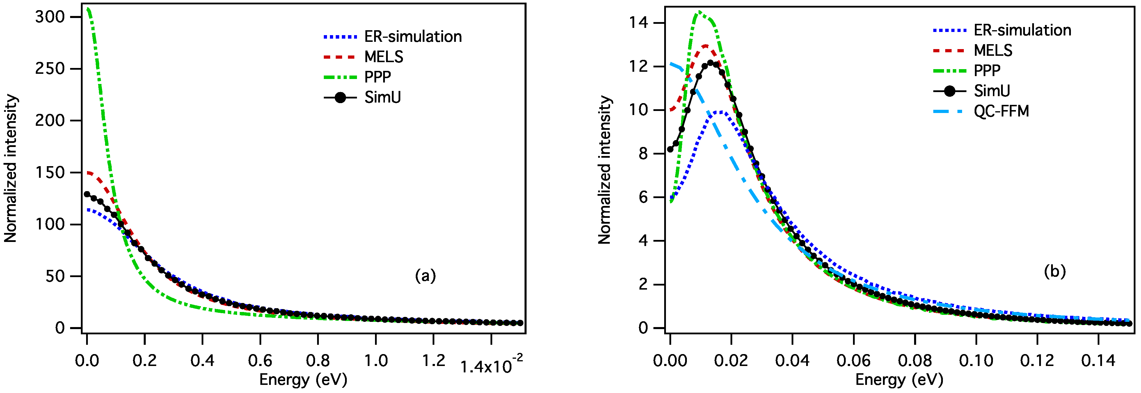
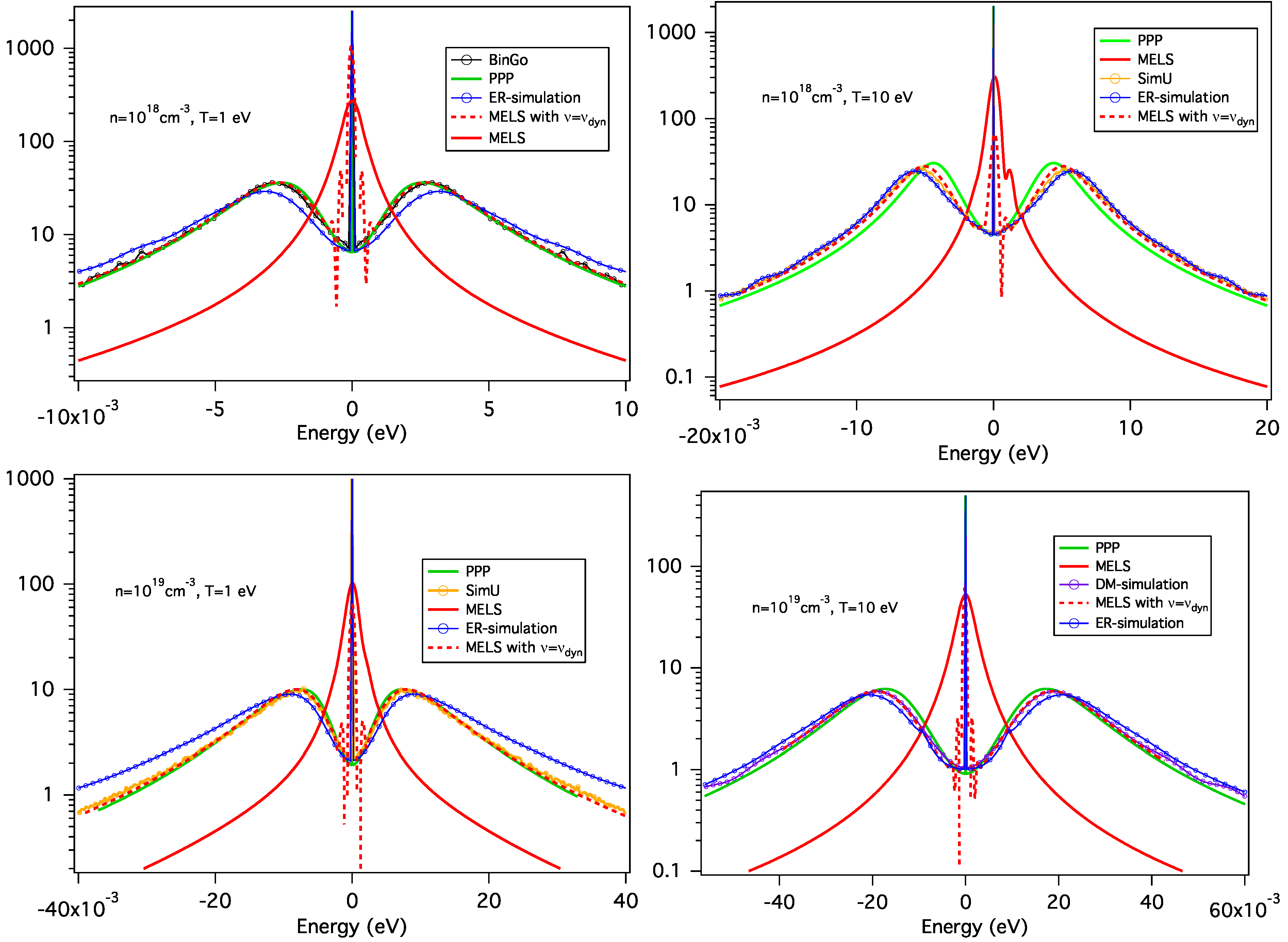
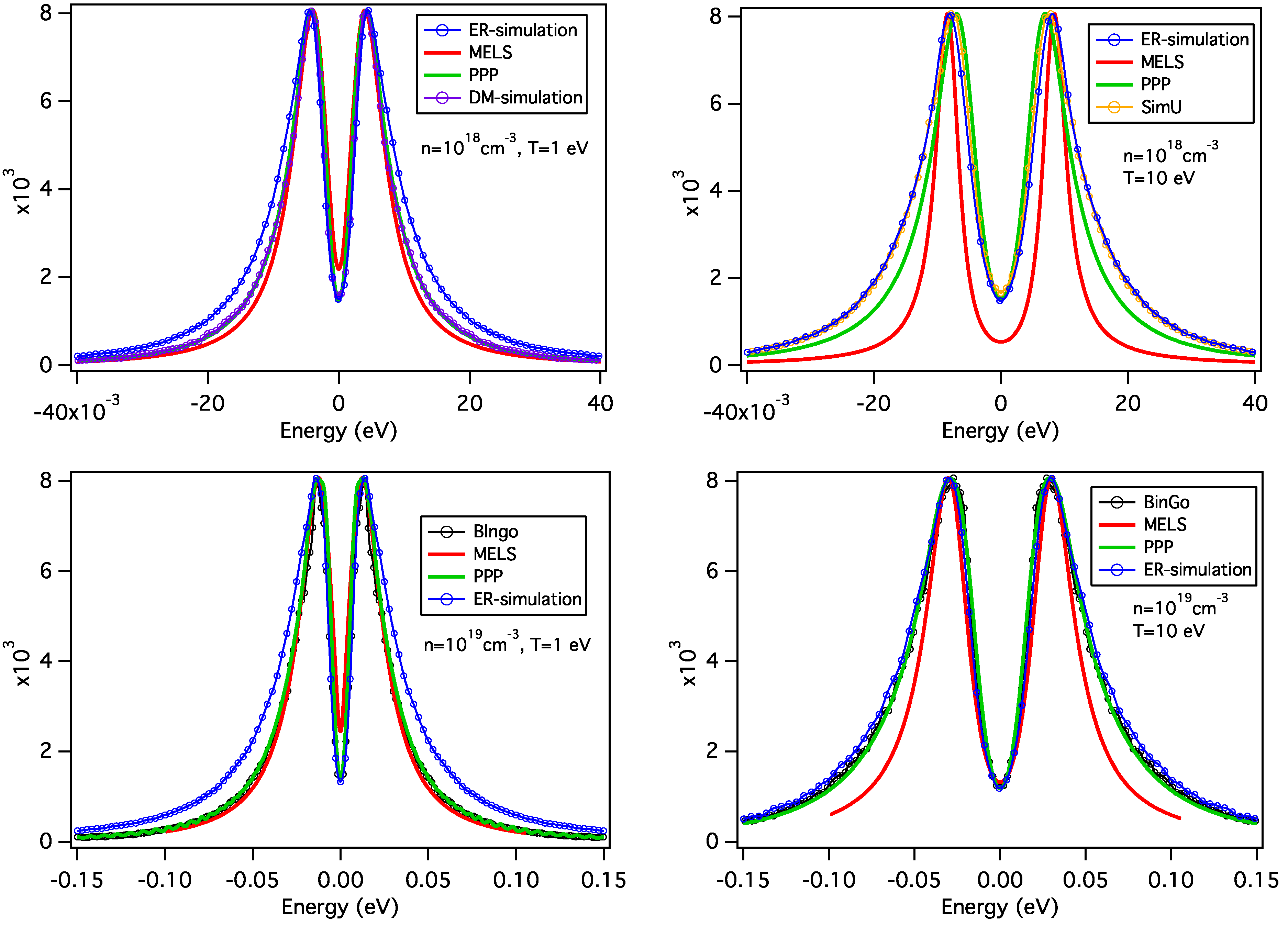
• The SimU code [11]: The perturbing fields are simulated by the particle field generator, where the motion of a finite number of plasma particles (electrons and ions) is calculated assuming that classical trajectories are valid. Then, using this field as a perturbation, the radiator dipole oscillating function is calculated by the Schrödinger solver. Finally, using the fast Fourier transformation (FFT) method, the power spectrum of the radiator dipole oscillating function is evaluated, giving the spectral line shape. The results of repeated runs of this procedure are then averaged to obtain a smooth spectrum. Although, in principle, the particle field generator may account for interactions between all particles, for the cases presented in this study, perturbing protons were modeled as reduced-mass Debye quasiparticles interacting only with the stationary radiator via the Debye potential.
• The BinGo code [12]: This code uses standard classical MD simulation to compute the perturbing fields. In this work, the plasma model consists of classical point ions interacting together through a Coulombic potential screened by electrons and localized in a cubic box with periodic boundary conditions. Newton’s equations of particle motion are integrated by using a velocity-Verlet algorithm using a time-step consistent with energy conservation. The simulated time-depending field histories are used in a step-by-step integration of the Schrödinger equation to obtain $U_l\left(t\right)$ and, thus, $C_{dd,l}\left(t\right)$ in the Liouville space. An average over a set of histories is necessary to evaluate $C_{dd}\left(t\right)$. Again, the spectral line shape is obtained using FFT.
• The Euler–Rodrigues (ER)-simulation code [13]: The plasma model for the simulation of time-dependent field histories consists of an emitter at rest in the center of a spherical volume and set in a bath of statistically independent charged quasi-particles moving along straight line trajectories. A reinjection technique ensures statistical homogeneity and stability. The simulated electric field histories are used in a solver for the evolution of the atomic system. For hydrogen, if the SO (4) symmetry is valid, Euler–Rodrigues (ER) parameters are used; otherwise the diagonalization process is done using Jacobi’s method.
• The DM-simulation code [14]: This code uses the same solver as the ER-simulation code, but the time-dependent field histories are simulated using the MD simulation technique in order to account for the particle interactions.

Even though these numerical simulation techniques have, successfully, been used as model laboratory experiments to compare with line shapes resulting from other method calculations or experiments, they can be impractical when the relevant atomic structure becomes too complex. Several approaches and models have been developed to overcome this difficulty [22] and implemented in numerical codes. Three different models (or codes) have contributed to the present study:

• The multi-electron line shape (MELS) code [24]: The “standard” theory (quasi-static ions and impact electrons) and the Boerker-Iglesias-Dufty (BID) model [15] to account for ion dynamics effects. The microfield distribution is from the adjustable-parameter exponential approximation (APEX) model [25,26].
• The PPP code [27]: The Stark broadening is taken into account in the framework of the standard theory by using the static ion approximation and an impact approximation for the electrons or including the effects of ionic perturber dynamics by using the fluctuation frequency model [16,17]. The microfield distribution functions required are calculated using the APEX model or an external MD simulation code.
• Quasicontiguous (QC)-frequency fluctuation model (FFM) [18,19]: The static line profile for a fixed field is represented by a rectangular shape, which is then integrated over the microfield distribution with the dynamic properties of microfields accounted for via FFM.

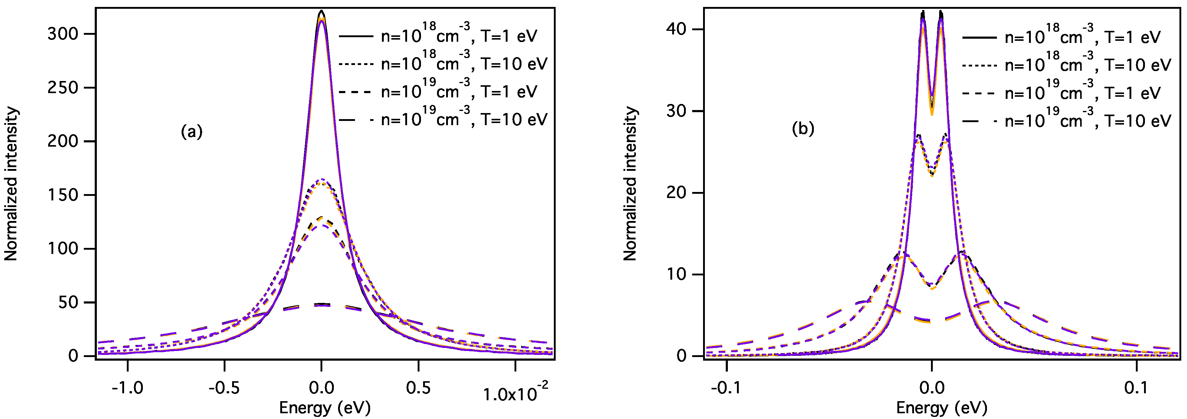
2.2. Plasma Characteristics

We consider a plasma containing an impurity (or a small percentage) of He II in protons at two temperatures, ($T=1$ and $T=10$ eV) and two ion number densities ($n={10}^{18}$ and $n={10}^{19}$ cm⁻³).

The plasma conditions are summarized in Table 1 together with some dimensionless parameters useful for characterizing the plasma, such as Γ, the coupling plasma parameter, α, the ratio of the interparticle distance to the screening length and typical frequency values, such as the plasma ion frequency, ${\omega }_{pi}$, and an estimate of the characteristic frequency of the perturbing field, ${\nu }_{dyn}$. With the interparticle distance and the screening length given by $r_0={(3/4\pi n)}^{1/3}$ and ${\displaystyle {\lambda }_D=\sqrt{\frac{k_{B}T}{4\pi n{e}^2}}}$, respectively, we have $\Gamma =e^2/\left(r_{0}kT\right)$, ${\displaystyle \alpha =\frac{r_0}{{\lambda }_D}}$, ${\displaystyle {\omega }_{\text{pi}}=\sqrt{\frac{4\pi n{e}^2}{m}}}$, m being the proton mass and ${\nu }_{dyn}=v/r_0$, where v is the thermal velocity in the radiator’s reference frame.

Table 1. Plasma characteristics.

Ne (cm−3)	T(eV)	Γ	α	ωpi (rad/s)	vdyn (rad/s)
1018	1	0.23	0.83	1.32 × 1012	1.77 × 1012
1018	10	0.02	0.26	-	5.57 × 1012
1019	1	0.50	1.22	4.16 × 1012	3.80 × 1012
1019	10	0.05	0.39	-	1.20 × 1013

Table 1. Plasma characteristics.

Ne (cm−3)	T(eV)	Γ	α	ωpi (rad/s)	vdyn (rad/s)
1018	1	0.23	0.83	1.32 × 1012	1.77 × 1012
1018	10	0.02	0.26	-	5.57 × 1012
1019	1	0.50	1.22	4.16 × 1012	3.80 × 1012
1019	10	0.05	0.39	-	1.20 × 1013

Figure 1a illustrates the temporal variation of the ionic field at the emitter for $n={10}^{18}$ cm⁻³ and T = 1 eV. In the same figure, the graph in the subwindow shows the field autocorrelation function, $C_{FF}\left(t\right)$ whose decay gives an estimate of the time scale of the field fluctuations. Figure 1b shows the corresponding rotational z-component (full line) and the vibrational fields (dash-dot).

Figure 1. (a) Temporal variation of the three components and correlation function (subwindow) of the perturbing ionic field; (b) temporal variation of the z-component of the rotational field (full line) and of the vibrational field (dash-dot line) at the emitter. The plasma conditions are $n={10}^{18}$ cm⁻³ and T = 1 eV for both (a) and (b).

Figure 1. (a) Temporal variation of the three components and correlation function (subwindow) of the perturbing ionic field; (b) temporal variation of the z-component of the rotational field (full line) and of the vibrational field (dash-dot line) at the emitter. The plasma conditions are $n={10}^{18}$ cm⁻³ and T = 1 eV for both (a) and (b).

The characteristic time scale of the field fluctuations has to be compared to the radiator time of interest, which is usually determined by the inverse of the HWHM (half width at half maximum) due to all broadening mechanisms of the considered line profile. This time depends on the plasma conditions and on the atomic data of the considered line and can be considered as the physical time of interest characterizing the response time of a plasma measurement device.

If the radiator time of interest is small compared to the time scale of the field fluctuations (HWHM⁻¹ ≪ ${\nu }_{dyn}^{-1}$, for example), the ion field varies little over the radiator time of interest and may be considered as a static field well characterized by a static field distribution function (quasi-static approximation). As soon as the two characteristic times are of the same order of magnitude, it becomes necessary to account for ion motion on the line profile.

The following results have been obtained for extreme conditions that allow for a better understanding of the differences observed for the various codes and methods. Two different lines have been chosen: the hydrogen-like helium Lyman-α and -β lines. The spectral line shapes of these two lines calculated in the framework of the quasi-static approximation are plotted in Figure 2 and compared to the results accounting for ion motion obtained with a simulation code. The width of the Lyman-α line ($n=2-n^{\prime }=1$) is very sensitive to the ion motion effect due to the unshifted central component, whereas the width of the Lyman-β line ($n=3-n^{\prime }=1$), which is broader than the Lyman-alpha, due to a largest upper principal quantum number and does not have unshifted central component, is less affected.

Figure 2. Spectral line shapes of the Lyman-α (a) and Lyman-β line (b) of hydrogen-like Helium calculated in a quasi-static (dash line) and in a fluctuating (full line) ionic electric field produced by protons at $n={10}^{19}$ cm⁻³ and T = 10 eV.

Figure 2. Spectral line shapes of the Lyman-α (a) and Lyman-β line (b) of hydrogen-like Helium calculated in a quasi-static (dash line) and in a fluctuating (full line) ionic electric field produced by protons at $n={10}^{19}$ cm⁻³ and T = 10 eV.

In the following, we will separately analyze how changing the direction and magnitude of the ionic electric field $\overrightarrow{F}\left(t\right)$ will influence the line shape. Comparisons between the different codes and methods are also performed.

3. Results

3.1. Generalities

Simulation results of the effects of the magnitude and direction fluctuations of the electric field on the Lyman-α line are plotted in Figure 3a,b, respectively, for $n={10}^{19}$ cm⁻³. It can be seen that the vibration of the electric field with a fixed direction (Figure 3a) does not affect the central component, whereas each lateral component tends to merge around its gravity center. As expected, the wings of the line are well reproduced by the static profile (the relevant times of interest in the line wings are small compared to the characteristic times of the field fluctuations). Increasing the temperature increases the fluctuation rate, but as the static line width also depends on temperature (due to the Debye-screened potential), the ratio between these two values does not change significantly, and the effects of vibrations on the profile are very similar. Concerning the pure rotating field case (Figure 3b), the situation is completely different. As the field has a fixed magnitude, $F_0$, the static profile is composed of three un-broadened Stark components, one central unshifted component and two lateral ones (in Figure 3b, the components have been broadened artificially to allow for plotting). When the fluctuations of the field are taken into account, the field magnitude is unchanged, only its direction fluctuates. Here, an increase of temperature results in an increase of dynamics effects. All the Stark components are affected by the field direction changes by being broadened and merged to the center of gravity.

Figure 3. Spectral line shapes of the Lyman-α line in a pure vibrating field (a) and a pure rotating field (b) compared to the corresponding static profiles, at $n={10}^{19}$ cm⁻³ and two temperatures, T = 1 and T = 10 eV. The dynamic case results have been obtained with the BinGo simulation code.

Figure 3. Spectral line shapes of the Lyman-α line in a pure vibrating field (a) and a pure rotating field (b) compared to the corresponding static profiles, at $n={10}^{19}$ cm⁻³ and two temperatures, T = 1 and T = 10 eV. The dynamic case results have been obtained with the BinGo simulation code.

In Figure 4, the Lyman-β line profiles calculated by numerical simulations have been plotted for the same conditions as previously. Here, again, the vibrations of the electric field affect the “blue” and “red” lateral components by merging them to their respective center of gravity. As has been already mentioned, the dynamics effects are less important in this case, because the static line-width is broader than in the previous case. In Figure 4b, the effects of the field direction changes on the line profile are shown for the two different temperatures and compared to the static profile. Here, there is no unshifted component, and the effects of fluctuations are to broaden the Stark components, filling progressively the dip between the two sets of Stark components.

To have a better idea of the pure dynamics effect, results corresponding to various reduced masses between radiator and perturbers (${\mu }_0$, $4{\mu }_0$ and $16{\mu }_0$) have been plotted in Figure 5 for the Lyman-α line at n = 10¹⁸ cm⁻³ and T = 10 eV. Here, ${\mu }_0=0.8$ is the reduced mass in the He-H⁺ center of mass frame.

It can be seen on the full profile (Figure 5a) that for the largest value of the reduced mass, the dynamics profile still presents a structure in the wings, and when the dynamics effects increase (when the reduced mass decreases), the line broadening increases and any structure disappears. If the reduced mass were smaller, we would see a narrowing of the profile. For the rotational profile (Figure 5b), this narrowing is already seen, for the reduced mass equals ${\mu }_0$. The full profile is a complex combination of both rotational and vibrational effects. The shape of the Ly-α and -β line center is determined mainly by the effects related to the rotation of the electric field. Therefore, proper consideration of these effects in the models seems to be one of the keys of the ion dynamics issue.

Figure 4. Spectral line shapes of the Lyman-β line in a pure vibrating field (a) and a pure rotating field (b) compared to the corresponding static profiles, at $n=1\times {10}^{19}$ cm⁻³ and two temperatures, T = 1 and T = 10 eV. The dynamic case results have been obtained with the BinGo simulation code.

Figure 4. Spectral line shapes of the Lyman-β line in a pure vibrating field (a) and a pure rotating field (b) compared to the corresponding static profiles, at $n=1\times {10}^{19}$ cm⁻³ and two temperatures, T = 1 and T = 10 eV. The dynamic case results have been obtained with the BinGo simulation code.

Figure 5. Reduced-mass effect on the Lyman-α line shape at $n={10}^{18}$ cm⁻³ and T = 10 eV in the three models of field (full (a); rotation (b) and vibration (c)). The color codes black, red and blue correspond to ${\mu }_0$, $4{\mu }_0$ and $16{\mu }_0$, respectively. The calculations have been done with the SimU simulation code.

Figure 5. Reduced-mass effect on the Lyman-α line shape at $n={10}^{18}$ cm⁻³ and T = 10 eV in the three models of field (full (a); rotation (b) and vibration (c)). The color codes black, red and blue correspond to ${\mu }_0$, $4{\mu }_0$ and $16{\mu }_0$, respectively. The calculations have been done with the SimU simulation code.

3.2. Code Comparisons

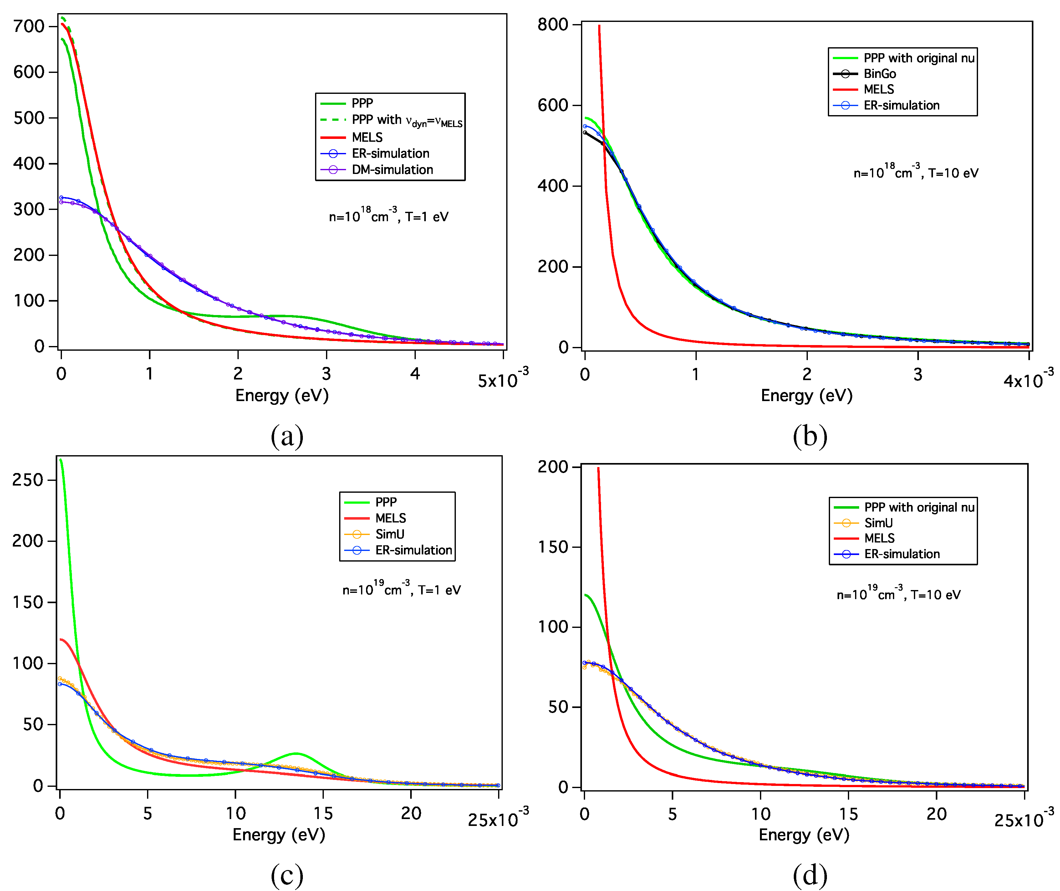
In this work, both MELS and PPP have been modified to account for vibration only.

The MELS code uses a stochastic microfield description of the plasma for the ion dynamics effect. The model obtains an exact solution for the line profile assuming an idealized stochastic process. It is possible to constrain the model by preserving known important properties of the actual problem by adjusting free parameters in the theory. For the present calculations, the free parameter, the fluctuation rate, was chosen to satisfy the ion impact limit, which, in principle, is equivalent to reproducing the short time limit of the momentum auto correlation function [24]. The rotational field fluctuations were computed by performing the integrations over the electric field directions as before [24], but at a single value of the field magnitude. The vibrational fluctuations were computed by restricting the angle average to a single field direction in the z-axis.

In the PPP code, the ion dynamics effects are treated by means of the frequency fluctuation model (FFM) [16,17]. The FFM is based on the premise that a quantum system perturbed by an electric microfield behaves like a set of field-dressed two-level transitions, the Stark dressed transitions. If the microfield is time varying, the transitions are subject to a collision-type mixing process—a Markov process—induced by the field fluctuations. In practice, the FFM line-shape is the result of intensity exchanges between different spectral domains of the static line-shape with an exchange rate given by ${\nu }_{dyn}$ (Table 1). Owing to the fact that a pure vibrational field will mix neither the central component with the lateral components nor the lateral components together, the code has been adapted in order to mix only the Stark components that must be mixed. For the rotational model, the static profile has been obtained by setting the electric field to $F_0{\overrightarrow{n}}_z$, and the usual “ion-dynamics” models, FFM, have been applied. It is the mixing of the static Stark components all together that mimics the direction changes of the electric field. The chosen mixing process is a Markov process, suggesting that the cause of the change in states is so violent, that in its final states, the system has no memory of its initial state.

3.2.1. Full Cases

In this example, the line profiles are calculated for the time-dependent field created by the protons interacting through an electron-screened Coulomb (i.e., Debye–Yukawa) potential. As a first observation, the three codes, BinGo, DM-simulation and SimU, give always very similar results (cf. Figure 6). The BinGo and DM-simulation codes are similar and account for all of the interactions between particles, whereas the SimU code simulates electron Debye-screened quasi-particles, which interact only with the charged emitter. A few minor differences appear in the center of the lines, within the uncertainties of the different methods. For instance, looking at the Lyman-α line (Figure 6a), the deviation maximum appears for $n={10}^{19}$ cm⁻³ and T = 1 eV and represents about 6% on the peak value. The numerical simulations, BinGo, DM-simulation and SimU, will then be considered as equivalent laboratory numerical experiments, and except for the line-width comparisons, results corresponding to these three simulations will be plotted only once, for clarity.

The results obtained for both lines, with the different codes, have been compared and plotted in Figure 7 for $n={10}^{19}$ cm⁻³ and T = 1 eV. It can be seen that the lines calculated by the ER-simulation code are too broad. In this code, the fields measured at the emitter are screened by electrons, but no particle interactions are taken into account (the particles move on straight-path trajectories); thus, the static field distribution function is shifted toward the large fields. This leads to broader static profiles and to changing the ratio between static and dynamic effects. The Stark profile is, in this case, less affected by ion dynamics effects. This behavior is more pronounced at low temperature when the plasma coupling parameter increases.

Figure 6. Spectral line shapes of the Lyman-α (a) and -β (b) line in a time-dependent field created by interacting protons. Comparisons of the results obtained by the three simulation codes: SimU (yellow), BinGo (black) and DM-simulation (purple).

Figure 6. Spectral line shapes of the Lyman-α (a) and -β (b) line in a time-dependent field created by interacting protons. Comparisons of the results obtained by the three simulation codes: SimU (yellow), BinGo (black) and DM-simulation (purple).

Figure 7. Spectral line shapes of the Lyman-α (a) and -β (b) line in a time-dependent field created by interacting protons at $n={10}^{19}$ cm⁻³ and T = 1 eV. Comparisons of the results obtained by the different codes.

Figure 7. Spectral line shapes of the Lyman-α (a) and -β (b) line in a time-dependent field created by interacting protons at $n={10}^{19}$ cm⁻³ and T = 1 eV. Comparisons of the results obtained by the different codes.

The PPP code qualitatively reproduces the same tendencies as simulation, but it underestimates the ion dynamics at the center of the line, whereas the wings are well reproduced. This could be related to a poor accounting for field direction fluctuation effects.

By construction, the QC-FFM does not show any dip at the center of the Lyman-beta line, but the wings are well represented and the line widths are consistent with those obtained using the FFM in the PPP code. Concerning the MELS code, the ion dynamics effects are well reproduced at T = 1 eV, but they are overestimated at T = 10 eV (see Figure 8).

Both codes, MELS and PPP, give similar answer to ion dynamics if their fluctuation rates ν are the same [24]. When ν increases, the line width is first increased; then, when ν becomes larger than the static line width, the line shape begins to narrow down and tends to the fast-fluctuation limit, which corresponds to ν = ∞. In this work, the PPP fluctuation rates, equal to ${\nu }_{dyn}$ (cf. Table 1), are always much smaller than the MELS ones. This is the reason why the same observation in Figure 8 (too small linewidth) can be due to different underlying causes (the dynamics effects are either too weak or too strong).

Figure 8. Full line widths at half maximum (FWHM) of the Lyman-α (a) and -β (b) line in a time-dependent field created by interacting protons versus temperature at $n={10}^{18}$ cm⁻³ (full lines) and $n={10}^{19}$ cm⁻³ (dashed lines). Comparisons of the results obtained by the different codes: BinGo (black), Euler–Rodrigues (ER)-simulation (blue), MELS (red), PPP (green), QC-frequency fluctuation model (FFM) (turquoise blue), SimU (yellow) and DM-simulation (purple).

Figure 8. Full line widths at half maximum (FWHM) of the Lyman-α (a) and -β (b) line in a time-dependent field created by interacting protons versus temperature at $n={10}^{18}$ cm⁻³ (full lines) and $n={10}^{19}$ cm⁻³ (dashed lines). Comparisons of the results obtained by the different codes: BinGo (black), Euler–Rodrigues (ER)-simulation (blue), MELS (red), PPP (green), QC-frequency fluctuation model (FFM) (turquoise blue), SimU (yellow) and DM-simulation (purple).

Figure 9. Spectral line shapes of the Lyman-α line in a pure vibrating field. Comparisons of the results obtained by the different codes.

Figure 9. Spectral line shapes of the Lyman-α line in a pure vibrating field. Comparisons of the results obtained by the different codes.

Figure 10. Spectral line shapes of the Lyman-β line in a pure vibrating field. Comparisons of the results obtained by different codes.

Figure 10. Spectral line shapes of the Lyman-β line in a pure vibrating field. Comparisons of the results obtained by different codes.

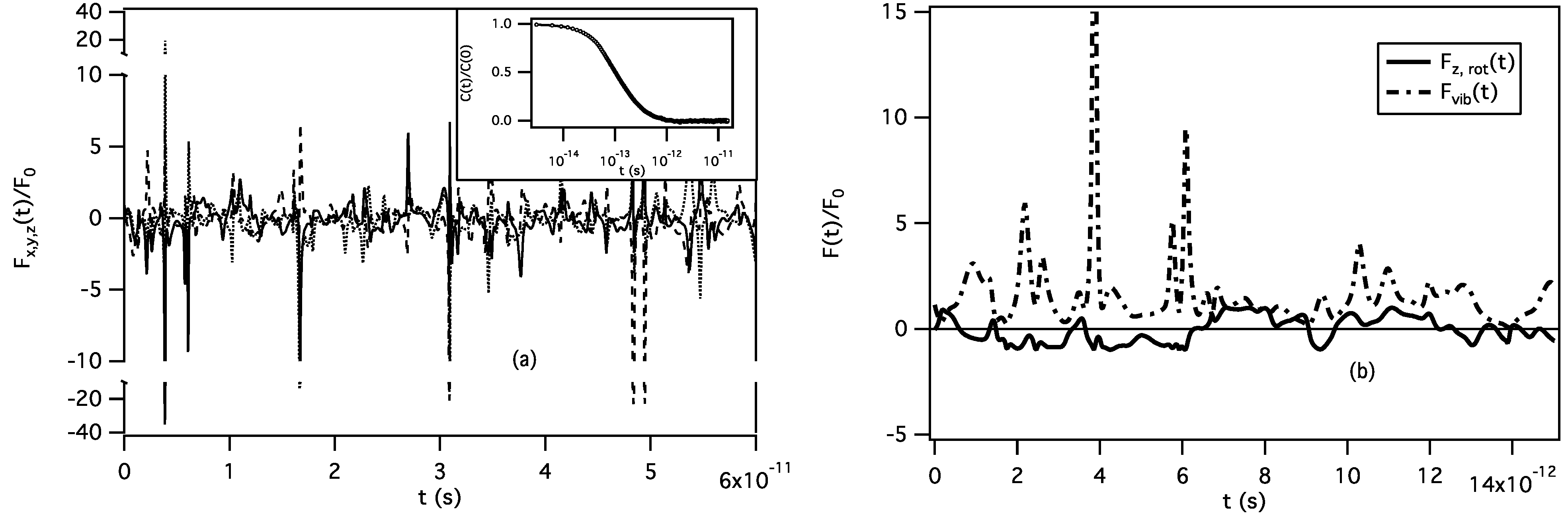
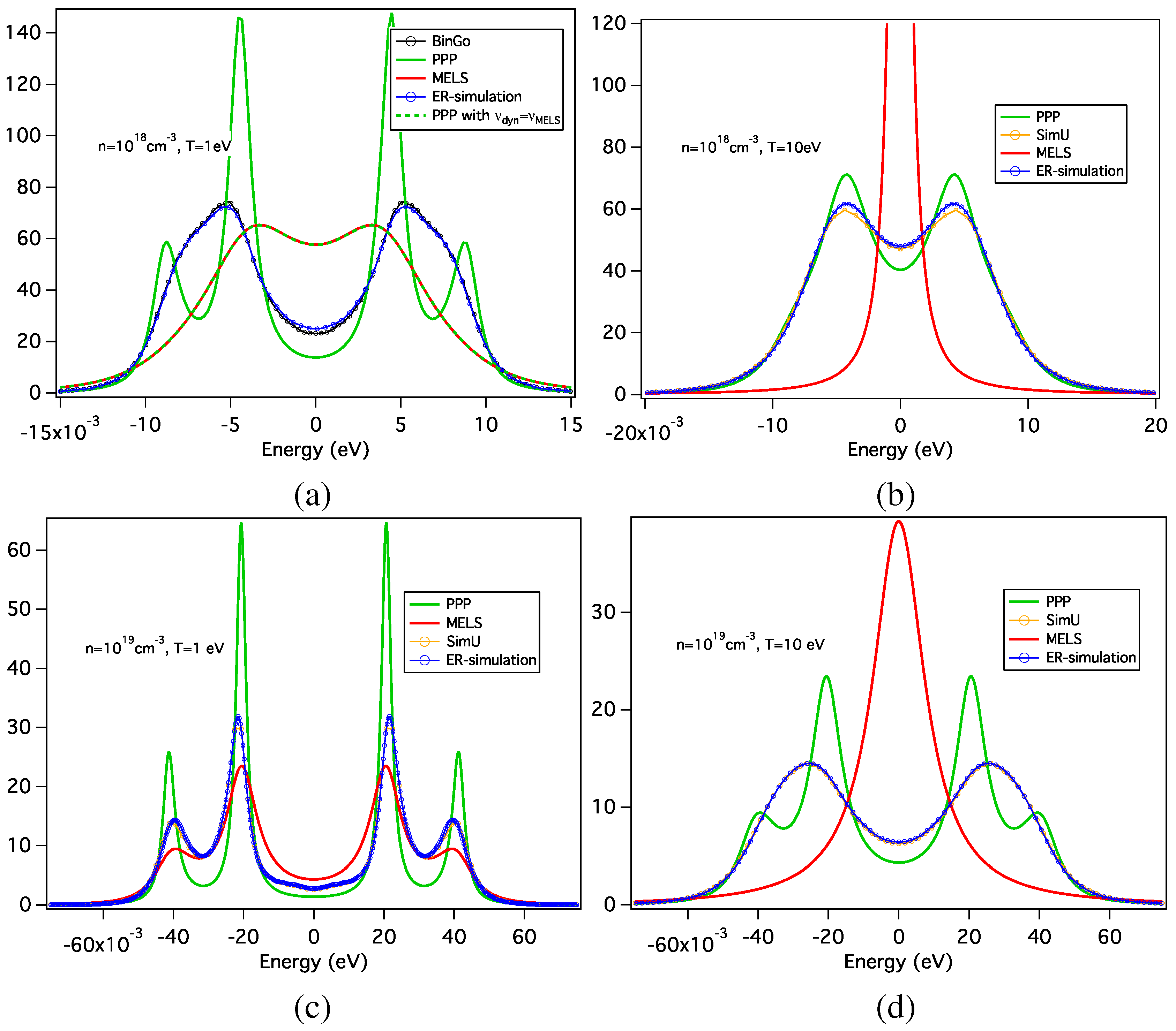
3.2.2. Vibration Case

In this section, calculations of the spectral profile have been performed assuming a pure vibrating field. Results for the Lyman-α and -β lines are plotted in Figure 9 and Figure 10, respectively.

At T = 1 eV, the results obtained with ER-simulation are noticeably different from other simulation results, because in these conditions, the correlation effects are important and are not taken into account in the model. PPP compares well with the simulations of reference. At T = 10 eV, the correlation effects are less pronounced and ER-simulation gives results very close to those of the reference simulations. The line profiles obtained with the PPP code are slightly too narrow, especially at low density. In all of the cases, MELS shows results slightly too narrow for the Lyman-β line and results radically different for the Lyman-α line. In MELS, if the fluctuation rate, ν, is set to ${\nu }_{dyn}$, the Lyman-α results compare very well with simulations, making abstraction of the central part of the lines. The central part of the lines presents a broadening, which could be attributed to the impact limit present in the BID model. For small ν, this broadening is small (leading to numerical noise on the profiles), and for larger ν, this broadening dominates.

According to these remarks, it appears that the FFM and BID with the same fluctuation rates mimic correctly the magnitude fluctuation effects on the profiles. The usual BID fluctuation rate is too large and leads to too strong field-fluctuation effects.

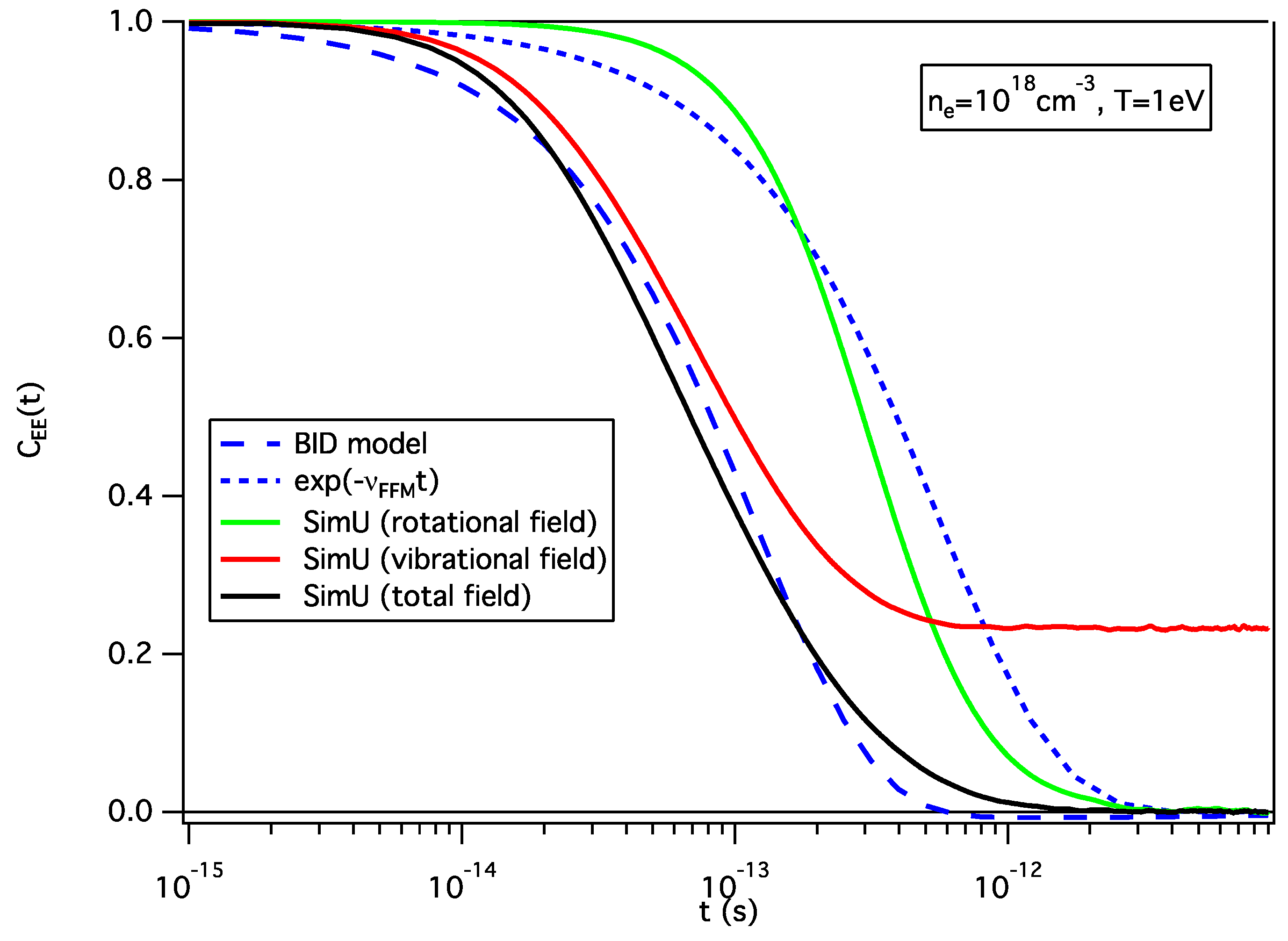
3.2.3. Rotation Case

The Lyman-α and -β line profiles calculated in a pure rotating field for different densities and temperatures have been plotted in Figure 11 and Figure 12, respectively. As the first result, it can be noticed that the ER-simulation code gives similar results as the reference simulations. Particle interactions have negligible effects on the line profiles in these cases. As an overall tendency, the PPP results appear to be too static and the MELS ones too dynamic. It is shown in Figure 11a and Figure 12a that with the same fluctuation rate, PPP and MELS give similar results. It has been checked that no fluctuation rate allows the reproducing of the simulation results. Except for the Lyman-α line at $n={10}^{18}$ cm⁻³ and T = 10 eV (cf. Figure 11b) where the rotational profile is well reproduced with the PPP fluctuation rate, PPP and MELS results will be too structured for a small fluctuation rate, and they will be too strongly merged to the line center for a large one. In these two codes, the implemented models to account for ion dynamics effects are both stochastic models: one describes the time-dependent field fluctuations (BID) and the other assumes a Markovian process for the fluctuations of emission radiation (FFM). If the BID fluctuation rate is constant, the two codes will give similar results. Even though they both give good approximation of the line shapes in realistic conditions (when all of the broadening effects are accounting for), both of them are unable to reproduce the rotational profiles in the framework of this study. It seems that the stochastic processes had to be chosen differently.

Figure 11. Spectral line shapes of the Lyman-α line in a pure rotating field. Comparisons of the results obtained by the different codes.

Figure 11. Spectral line shapes of the Lyman-α line in a pure rotating field. Comparisons of the results obtained by the different codes.

Figure 12. Spectral line shapes of the Lyman-β line in a pure rotating field. Comparisons of the results obtained by the different codes.

Figure 12. Spectral line shapes of the Lyman-β line in a pure rotating field. Comparisons of the results obtained by the different codes.

4. Discussion

Our goal in this paper has been to investigate the reasons of the big differences, which appeared in spectral line shape models intended to account for ionic field fluctuation effects (well-known as ion dynamics effects) in the framework of the first SLSP workshop held in Vienna in 2012. For this purpose, a separate study of the magnitude and direction fluctuation effects on two different spectral lines in plasma conditions chosen in order to perform severe tests on models has been performed. All the simulation codes accounting for interactions between particles or using quasi-particles interacting with the emitter give similar results. They have been taken as benchmarks. These simulation results show that the central part of the line profiles is mainly affected by rotational effects, and a good representation of these effects seems to be the clue of the ion dynamics problem. The simulation codes using quasi-particle on straight-path trajectory models, which are very economical in terms of computing time, give the right answer concerning the rotation effects, but the full profiles are too broad, due to a too large static Stark splitting for both cases at T = 1eV (Γ = 0.23 and Γ = 0.5, respectively), where the effects of interactions between particles are non-negligible. In this context, the intermediate approach employed by SimU in the present study, i.e., accounting only for the radiator-perturber interactions, appears to provide good accuracy with only a minor (relative to the straight-path-trajectory model) increase of the computational time. Evidently, such an approach becomes questionable for strongly-coupled plasmas (Γ ≳ 1).

The codes based on stochastic models do not reproduce correctly the rotation effects, even though they are known to give a good approximation of the profiles in realistic conditions [28]. Figure 7 shows a rather good agreement between MELS and simulation results; the fluctuation rate used in PPP is too small and results in too static profiles. PPP would give similar results as MELS if the MELS fluctuation rate were used. We recall that the PPP and MELS codes were both developed for complex atomic systems, such as multielectron ions found in hot, dense laser-produced plasma. Thus, they have to find a satisfactory compromise between accuracy and efficiency. For a better understanding of the differences with simulations, a comparison of the different field autocorrelation functions has been plotted in Figure 13 for $n={10}^{18}$ cm⁻³ and T = 1 eV. The total, rotational and vibrational field autocorrelation functions obtained with the SimU simulation code have been plotted together with the total field correlation function corresponding to the BID model (cf. Appendix A) and an exponential function with a decay rate equal to ${\nu }_{dyn}$. The absolute value of the rotational-field autocorrelation function is, by construction, $F_0^2$, while that of the vibrational- and total-field ones is 3/Γ-times larger [29]. The vibrational field correlation function shows a plateau at the long time limit due to a non-null value of the mean vibrational field. Even though the correlation function models seem to be rather good approximations, the corresponding profiles do not coincide with the simulations. It has been verified that changing the fluctuation rate is not relevant.

Figure 13. Autocorrelation functions of the total (black line), rotational (green line) and vibrational (red line) fields compared to the BID model correlation function (dashed blue line) and the exponential function corresponding to the FFM model (short dashed blue line).

Figure 13. Autocorrelation functions of the total (black line), rotational (green line) and vibrational (red line) fields compared to the BID model correlation function (dashed blue line) and the exponential function corresponding to the FFM model (short dashed blue line).

It seems that the underlying stochastic models intended to account for ion dynamics are inappropriate for mimicking the pure rotating field. Other choices could be made. For instance, instead of working in the framework of strong collision models with constant fluctuation rates, a model with a frequency-dependent fluctuation rate or a diffusion model on the basis of what has been done for Doppler profiles [30] could be tested.

References

1. Dufty, J. Ion motion in plasma line broadening. Phys. Rev. A 1970, 2, 534–541. [Google Scholar] [CrossRef]
2. Frisch, U.; Brissaud, A. Theory of Stark broadening—I soluble scalar model as a test. J. Quant. Spectrosc. Radiat. Transf. 1971, 11, 1753–1766. [Google Scholar] [CrossRef]
3. Brissaud, A.; Frisch, U. Theory of Stark broadening—II exact line profile with model microfield. J. Quant. Spectrosc. Radiat. Transf. 1971, 11, 1767–1783. [Google Scholar] [CrossRef]
4. Hey, J.D.; Griem, H.R. Central structure of low-n Balmer lines in dense plasmas. Phys. Rev. A 1975, 12, 169–185. [Google Scholar] [CrossRef]
5. Demura, A.V.; Lisitsa, V.S.; Sholin, G.V. Effect of reduced mass in Stark broadening of hydrogen lines. Sov. Phys. J. Exp. Theor. Phys. 1977, 46, 209–215. [Google Scholar]
6. Kelleher, D.E.; Wiese, W.L. Observation of ion motion in hydrogen Stark profiles. Phys. Rev. Lett. 1973, 31, 1431–1434. [Google Scholar] [CrossRef]
7. Wiese, W.L.; Kelleher, D.E.; Helbig, V. Variations in Balmer-line Stark profiles with atom-ion reduced mass. Phys. Rev. A 1975, 11, 1854–1864. [Google Scholar] [CrossRef]
8. Stamm, R.; Voslamber, D. On the role of ion dynamics in the stark broadening of hydrogen lines. J. Quant. Spectrosc. Radiat. Transf. 1979, 22, 599–609. [Google Scholar] [CrossRef]
9. Stambulchik, E. Review of the 1st spectral line shapes in plasmas code comparison workshop. High Energy Density Phys. 2013, 9, 528–534. [Google Scholar] [CrossRef]
10. Spectral Line Shapes in Plasmas code comparison workshop. Available online: http://plasma-gate.weizmann.ac.il/slsp/ (accessed on 30 May 2014).
11. Stambulchik, E.; Maron, Y. A study of ion-dynamics and correlation effects for spectral line broadening in plasma: K-shell lines. J. Quant. Spectrosc. Radiat. Transf. 2006, 99, 730–749. [Google Scholar] [CrossRef]
12. Talin, B.; Dufour, E.; Calisti, A.; Gigosos, M.A.; González, M.A.; del Río Gaztelurrutia, T.; Dufty, J.W. Molecular dynamics simulation for modelling plasma spectroscopy. J. Phys. A Math. Gen. 2003, 36, 6049. [Google Scholar] [CrossRef]
13. Gigosos, M.A.; Cardeñoso, V. New plasma diagnosis tables of hydrogen Stark broadening including ion dynamics. J. Phys. B: At. Mol. Opt. 1996, 29, 4795–4838. [Google Scholar] [CrossRef]
14. Lara, N. Cálculo de espectros Stark de plasmas fuertemente acoplados mediante simulación de dinámica molecular. Ph.D. Thesis, University of Valladolid, Valladolid, Spain, 2013. [Google Scholar]
15. Boercker, D.B.; Iglesias, C.A.; Dufty, J.W. Radiative and transport properties of ions in strongly coupled plasmas. Phys. Rev. A 1987, 36, 2254–2264. [Google Scholar] [CrossRef] [PubMed]
16. Talin, B.; Calisti, A.; Godbert, L.; Stamm, R.; Lee, R.W.; Klein, L. Frequency-fluctuation model for line-shape calculations in plasma spectroscopy. Phys. Rev. A 1995, 51, 1918–1928. [Google Scholar] [CrossRef] [PubMed]
17. Calisti, A.; Mossé, C.; Ferri, S.; Talin, B.; Rosmej, F.; Bureyeva, L.A.; Lisitsa, V.S. Dynamic Stark broadening as the Dicke narrowing effect. Phys. Rev. E 2010, 81, 016406:1–016406:6. [Google Scholar] [CrossRef]
18. Stambulchik, E.; Maron, Y. Stark effect of high-n hydrogen-like transitions: quasi-contiguous approximation. J. Phys. B: At. Mol. Opt. 2008, 41, 095703. [Google Scholar] [CrossRef]
19. Stambulchik, E.; Maron, Y. Quasicontiguous frequency-fluctuation model for calculation of hydrogen and hydrogenlike Stark broadened line shapes in plasmas. Phys. Rev. E 2013, 87, 053108:1–053108:8. [Google Scholar] [CrossRef]
20. Baranger, M. Atomic and Molecular Processes; Bates, D.R., Ed.; Academic: New York, NY, USA, 1964. [Google Scholar]
21. Fano, U. Pressure Broadening as a Prototype of Relaxation. Phys. Rev. 1963, 131, 259–268. [Google Scholar] [CrossRef]
22. Griem, H. Principles of Plasma Spectroscopy; Cambridge University Press: Cambridge, UK, 1997. [Google Scholar]
23. Griem, H.R. Spectral Line Broadening by Plasmas; Academic: New York, NY, USA, 1974. [Google Scholar]
24. Iglesias, C.A. Efficient algorithms for stochastic Stark-profile calculations. High Energy Density Phys. 2013, 9, 209–221. [Google Scholar] [CrossRef]
25. Iglesias, C.A.; DeWitt, H.E.; Lebowitz, J.L.; MacGowan, D.; Hubbard, W.B. Low-frequency electric microfield distributions in plasmas. Phys. Rev. A 1985, 31, 1698–1702. [Google Scholar] [CrossRef] [PubMed]
26. Iglesias, C.A.; Rogers, F.J.; Shepherd, R.; Bar-Shalom, A.; Murillo, M.S.; Kilcrease, D.P.; Calisti, A.; Lee, R.W. Fast electric microfield distribution calculations in extreme matter conditions. J. Quant. Spectrosc. Radiat. Transf. 2000, 65, 303–315. [Google Scholar] [CrossRef]
27. Calisti, A.; Khelfaoui, F.; Stamm, R.; Talin, B.; Lee, R.W. Model for the line shapes of complex ions in hot and dense plasmas. Phys. Rev. A 1990, 42, 5433–5440. [Google Scholar] [CrossRef] [PubMed]
28. Ferri, S.; Calisti, A.; Mossé, C.; Rosato, J.; Talin, B.; Alexiou, S.; Gigosos, M.A.; González, M.A.; González, D.; Lara, N.; Gomez, T.; Iglesias, C.; Lorenzen, S.; Mancini, R.; Stambulchik, E. Ion dynamics effect on Stark broadened line shapes: A cross comparison of various models. Atoms. 2014, 2, 1–20. [Google Scholar]
29. Iglesias, C.A.; Lebowitz, J.L.; MacGowan, D. Electric microfield distributions in strongly coupled plasmas. Phys. Rev. A 1983, 28, 1667–1672. [Google Scholar] [CrossRef]
30. Rautian, S.G.; Sobel’man, I.I. The effect of collisions on the Doppler broadening of spectral lines. Soviet Phys. Uspekhi 1967, 9, 701–716. [Google Scholar] [CrossRef]