Scalar Aharonov–Bohm Phase in Ramsey Atom Interferometry under Time-Varying Potential

Abstract

In a Ramsey atom interferometer excited by two electromagnetic fields, if atoms are under a time-varying scalar potential during the interrogation time, the phase of the Ramsey fringes shifts owing to the scalar Aharonov–Bohm effect. The phase shift was precisely examined using a Ramsey atom interferometer with a two-photon Raman transition under the second-order Zeeman potential, and a formula for the phase shift was derived. Using the derived formula, the frequency shift due to the scalar Aharonov–Bohm effect in the frequency standards utilizing the Ramsey atom interferometer was discussed.

1. Introduction

The Ramsey resonance excited by two separated electromagnetic fields—originally described by Ramsey [1] and now understood as a kind of atom interferometer [2,3]—is used as a powerful tool for high-resolution laser spectroscopy [4] and high-precision measurement in fundamental physics [5]. In particular, this method has contributed to realizing the present primary time and frequency standards [6], where an atom in a superposition of two states exists in a zone during the interrogation time between two pulses, which is used to improve the spectral resolution to an ultimate value. However, during the interrogation time, atoms are also subjected to various time-varying scalar potentials from the surrounding environment.

In 1959, Aharonov and Bohm predicted that the phase of an atomic wave function in quantum mechanics shifts under a time-dependent homogeneous scalar potential [7]. This effect—now called the scalar Aharonov–Bohm effect—was originally proposed for electrons in a time-varying electric field, but is practically verified using neutral particles with a magnetic moment in a time-varying magnetic field (for example, neutrons [8] and hydrogen atoms [9]). In a Ramsey atom interferometer under a time-varying scalar potential, the phase of the Ramsey fringe shifts, since atoms with different magnetic quantum numbers are subjected to different scalar Aharonov–Bohm effects. We demonstrated the nondispersivity of this effect using a Ramsey atom interferometer with a two-photon Raman transition [10,11], and succeeded in measuring the phase shift due to the weak second-order Zeeman effect using the scalar Aharonov–Bohm phase [12]. In these experiments, the strength of the magnetic field was the same at the first and second interaction times when atoms were excited by the electromagnetic field, and it was changed by a fixed amount during the interrogation time. However, in the case of an actual time-varying potential, the resonance frequencies at two interaction times will be different, and the most probable frequency of the Ramsey fringes will be affected by the phase shift due to the scalar Aharonov–Bohm effect during the interrogation time. To the best of our knowledge, there have been no reports describing such a resonance condition of Ramsey fringes.

As reported in this paper, we investigate the frequency and phase shifts of a Ramsey atom interferometer under a time-varying potential and derive an empirical formula. Finally, we present a method of evaluating the uncertainty of the present primary atomic clock due to the scalar Aharonov–Bohm effect.

2. Principle

Consider a typical Ramsey atom interferometer, as shown in Figure 1. In Ramsey interferometry, atoms in the ground state undergo a transition to a long-lived excited state by applying two separated oscillatory fields with the resonance frequency between the two states. Ideally, the atoms in the ground state are irradiated by two π/2 pulses with duration τ, which are separated by time T. After the second pulse, the transition probability of atoms to the excited state is generally given by [13]

$$P=2\left\{{\cos }^2\left(\frac{\mathsf{\Omega }\tau }{2}\right)+\frac{{\mathsf{\Omega }}_3^2}{{\mathsf{\Omega }}^2}{\sin }^2\left(\frac{\mathsf{\Omega }\tau }{2}\right)\right\}\frac{{\mathsf{\Omega }}_{\text{eff}}^2}{{\mathsf{\Omega }}^2}{\sin }^2\left(\frac{\mathsf{\Omega }\tau }{2}\right)\left\{1+\cos \left({\mathsf{\Omega }}_{3}T+{\phi }_1-{\phi }_2\right)\right\}$$

(1)

where Ω_eff is the effective angular Rabi frequency, Ω₃ = 2π(ν_L − ν₀) is the detuning angular frequency between the field frequency ν_L and resonance frequency ν₀, and Ω = $\sqrt{{\mathsf{\Omega }}_{\text{eff}}^2+{\mathsf{\Omega }}_3^2}$. ϕ₁ and ϕ₂ are the optical phases of the two pulses. When Ω_eff << Ω₃ and ϕ₁ = ϕ₂, Equation (1) is approximated to

$$\begin{array}{l}P=\frac{1}{2}{\mathsf{\Omega }}_{eff}^2{\tau }^2{\text{sinc}}^2\left(\pi ({\nu }_L-{\nu }_0)\tau \right)\left[1+\cos \left\{2\pi ({\nu }_L-{\nu }_0)(\tau +T)\right\}\right]\\ \equiv f({\nu }_L-{\nu }_0)\left[1+\cos \left\{2\pi ({\nu }_L-{\nu }_0)(\tau +T)\right\}\right]\end{array}$$

(2)

where f is the envelope curve of the transition probability as a function of the detuning frequency, and the last term represents Ramsey fringes whose cycle is 1/(τ + T). When the field frequency ν_L is tuned to the resonance frequency ν₀, the peak of the Ramsey fringes coincides with the center frequency of the envelope.

We consider the case where the atom interferometer is under a time-varying scalar potential V(t). Then, Equation (2) is given by

$$\begin{array}{c}P=\left\{{\cos }^2\left(\frac{\mathsf{\Omega }\tau }{2}\right)+\frac{{\mathsf{\Omega }}_3^2}{{\mathsf{\Omega }}^2}{\sin }^2\left(\frac{\mathsf{\Omega }\tau }{2}\right)\right\}\frac{{\mathsf{\Omega }}_{\text{eff}}^2}{{{\mathsf{\Omega }}^{\prime }}^2}{\sin }^2\left(\frac{{\mathsf{\Omega }}^{\prime }\tau }{2}\right)+\left\{{\cos }^2\left(\frac{{\mathsf{\Omega }}^{\prime }\tau }{2}\right)+\frac{{{\mathsf{\Omega }}^{\prime }}_3^2}{{{\mathsf{\Omega }}^{\prime }}^2}{\sin }^2\left(\frac{{\mathsf{\Omega }}^{\prime }\tau }{2}\right)\right\}\frac{{\mathsf{\Omega }}_{\text{eff}}^2}{{\mathsf{\Omega }}^2}{\sin }^2\left(\frac{\mathsf{\Omega }\tau }{2}\right)\\ +2\left\{\cos \left(\frac{\mathsf{\Omega }\tau }{2}\right)\cos \left(\frac{{\mathsf{\Omega }}^{\prime }\tau }{2}\right)-\frac{{\mathsf{\Omega }}_3{{\mathsf{\Omega }}^{\prime }}_3}{\mathsf{\Omega }{\mathsf{\Omega }}^{\prime }}\sin \left(\frac{\mathsf{\Omega }\tau }{2}\right)\sin \left(\frac{{\mathsf{\Omega }}^{\prime }\tau }{2}\right)\right\}\frac{{\mathsf{\Omega }}_{\text{eff}}^2}{\mathsf{\Omega }{\mathsf{\Omega }}^{\prime }}\sin \left(\frac{\mathsf{\Omega }\tau }{2}\right)\sin \left(\frac{{\mathsf{\Omega }}^{\prime }\tau }{2}\right)\cos \left(\frac{{\mathsf{\Omega }}_3+{{\mathsf{\Omega }}^{\prime }}_3}{2}T+{\varphi }_1-{\varphi }_2\right)\\ -2\left\{\frac{{\mathsf{\Omega }}_3}{\mathsf{\Omega }}\sin \left(\frac{\mathsf{\Omega }\tau }{2}\right)\cos \left(\frac{{\mathsf{\Omega }}^{\prime }\tau }{2}\right)-\frac{{{\mathsf{\Omega }}^{\prime }}_3}{{\mathsf{\Omega }}^{\prime }}\cos \left(\frac{\mathsf{\Omega }\tau }{2}\right)\sin \left(\frac{{\mathsf{\Omega }}^{\prime }\tau }{2}\right)\right\}\frac{{\mathsf{\Omega }}_{\text{eff}}^2}{\mathsf{\Omega }{\mathsf{\Omega }}^{\prime }}\sin \left(\frac{\mathsf{\Omega }\tau }{2}\right)\sin \left(\frac{{\mathsf{\Omega }}^{\prime }\tau }{2}\right)\sin \left(\frac{{\mathsf{\Omega }}_3+{{\mathsf{\Omega }}^{\prime }}_3}{2}T+{\varphi }_1-{\varphi }_2\right)\end{array}$$

(3)

where Ω, Ω_eff and Ω₃ are for the first pulse and Ω′, Ω′_eff and Ω′₃ are for the second pulse. This equation is approximated to

$$P=g\left({\nu }_{\mathrm{L}}-{\nu }_0,V(0)/h,V(\tau +T)/h\right)\left[1+\cos \left\{2\pi ({\nu }_L-{\nu }_0)(\tau +T)-\frac{1}{\hslash }{\displaystyle {\int }_0^{\tau +T}V(t)dt}\right\}\right]$$

(3’)

where V(0)/h and V(τ + T)/h are the frequency shifts due to the dynamical potential at t = 0 and t = τ + T, respectively, and h is Planck’s constant. The function g is

$$g({\nu }_L-{\nu }_0,V(0)/h,V(\tau +T)/h)=\sqrt{f\left({\nu }_{\mathrm{L}}-{\nu }_0-V(0)/h\right)f\left({\nu }_{\mathrm{L}}-{\nu }_0-V(\tau +T)/h\right)}$$

(4)

Here, we assume that |V(0)/h − V(τ + T)/h| is sufficiently smaller than the width of the envelope, and that the π/2 pulse with duration τ is sufficiently short. Therefore, the width of envelope g is a slightly greater than that of f. The potential is assumed to be constant during the pulse width τ. During time T, the atoms are in a superposition state of the ground and excited states, and are subjected to a time-varying scalar potential. The integral term in the cosine function is the scalar Aharonov–Bohm phase, which is accumulated during time T. At the center frequency of the envelope curve—namely, ${\nu }_{\mathrm{L}}={\nu }_0+(V(0)+V(\tau +T))/(2h)$—the phase of the Ramsey fringe is given by

$$\phi =\frac{V(0)+V(\tau +T)}{2\hslash }(\tau +T)-\frac{1}{\hslash }{\displaystyle {\int }_0^{\tau +T}V(t)dt}$$

(5)

3. Experimental

In the present experiment, we used a Ramsey atom interferometer with two-photon Raman pulses, instead of rf pulses [14]. The experimental apparatus and setup were almost the same as those described in detail in our previous papers [12,15]. The time-domain Ramsey atom interferometer was composed of two ground hyperfine spin states of a cold sodium atom ensemble. A partial energy diagram of the sodium atom is shown in Figure 2a. The F = 1 and F = 2 states in the ground hyperfine structure of 3S_1/2 were coupled with circularly-polarized copropagating two-photon stimulated Raman pulses. The laser beam for the Raman pulse with a wavelength of 589 nm oscillating from a frequency-stabilized dye laser was detuned by about 500 MHz below the resonance frequency between the F = 2 state and the upper P_3/2, F’ = 2 state to suppress the Rayleigh scattering. It was phase-modulated by an electro-optical modulator (EOM) driven by a radio-frequency (rf) field with a frequency of about ν_HFS = 1.771626 GHz, which corresponds to the ground hyperfine energy splitting of sodium. The two-photon Raman pulse was composed of a carrier frequency and a 1st-order sideband frequency generated by the EOM. In the present experiment, the rf frequency of the synthesizer was stabilized within a few Hertz to a commercial rubidium atomic clock as a reference signal. The frequency difference between two Raman pulses was swept around the resonance frequency ν₀ for each measurement. The alternating current (AC) Stark frequency shift due to the two-photon Raman laser beam was cancelled out by adjusting the intensity ratio between the two frequencies [12].

The experimental setup is shown in Figure 2b. The sodium atoms that effused from an oven were decelerated by a Zeeman slower and trapped in a vacuum chamber (10⁻⁹ Pa) by a dual magneto–optical trap (MOT) [16]. To remove the stray magnetic field at the center area, we used three mutually orthogonal Helmholtz coils. Additionally, an anti-Helmholtz coil was used to compensate the weak inhomogeneous magnetic field parallel to the direction of the atomic beams (x-axis). Then they were cooled to about 120 μK by polarization gradient cooling (PGC). At a few milliseconds after the release of atoms from the trap, a quantization magnetic field was applied in the direction parallel to the z-axis, to resolve a degeneracy of an ensemble of cold atoms. The cold atoms were initialized to the F = 1 state by an initializing beam. After that, atoms were irradiated by two rectangular Raman pulses with a pulse area of π/2 separated by the interference time T to construct the Ramsey interferometer. Raman pulses with circular σ⁺ polarization were propagated parallel to the direction of the quantization magnetic field. At the quantization magnetic field of 10 μT, the three spectra of the σ⁺ – σ⁺ transitions were resolved with adjacent separation frequencies of 140 kHz. In this paper, we investigate the Ramsey fringes of the magnetic field insensitive 0 → 0 clock transition. The transition probability to the F = 2 was measured using the probe beam described in our previous paper [15].

4. Results and Discussion

4.1. Ramsey Atom Interferometer

To precisely measure the phase shift, we first checked how well Equation (2) can describe Ramsey fringes. Typical Ramsey fringes obtained at τ = 100 μs and T = 900 μs are shown in Figure 3a, where 16 fringes are observed in a frequency range of 16 kHz. These fringes were well-fitted by the function $f({\nu }_L-{\nu }_0)\left[1+\cos \left\{2\pi ({\nu }_L-{\nu }_0)T_{\text{eff}}\right\}\right]$, where T_eff is an effective interrogation time, as shown in a solid curve. The T_eff was obtained to be 1011 ± 2 μs, which was nearly equal to τ + T. This relationship was examined for several different τ and T, as shown in Figure 3b. It was found that, if τ < (τ + T)/10, the Ramsey cycle is equal to 1/(τ + T) within an uncertainty of 2%. For a longer T, T_eff is closer to τ + T. Therefore, Equation (2) holds. Furthermore, we also changed the duration of the two pulses τ₁ and τ₂, and we found the relationship T_eff = τ₁/2 + T + τ₂/2. We conclude that T_eff (which determines the Ramsey cycle) is determined by the time from the center of the first pulse to the center of the second pulse if τ₁ and τ₂ are shorter than T/10. Hereafter, in the present paper, the origin of the time was set at the center of the first pulse.

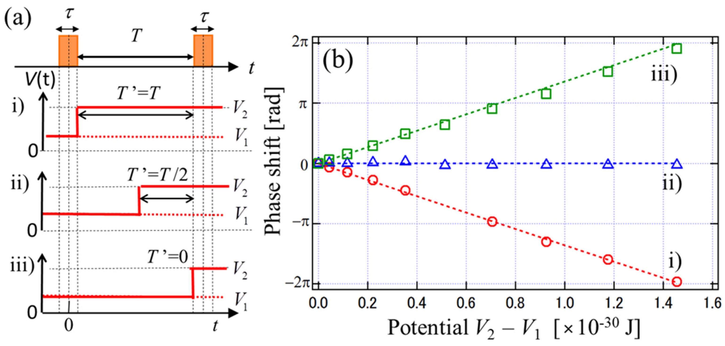
4.2. Scalar Aharonov–Bohm Phase

The resonance frequency of the clock transition between the m_F = 0 and m_F′ = 0 hyperfine states is perturbed by the second-order Zeeman effect and shifts by

$$\frac{V}{h}\equiv \Delta \nu =\frac{{(g_J-g_I)}^2{\mu }_B^2}{2h^2{\Delta }_{hfs}}{B}^2\equiv 0.22183\times {(B/\mathsf{\mu }\mathrm{T})}^2$$

(6)

where B is the strength of the quantization magnetic field, g_J and g_I are the fine structure and nuclear Landé g factors, respectively, μ_B is the Bohr magneton, and Δ_hfs is the hyperfine splitting frequency [12]. It was confirmed that the frequency of the resonance curve shifts in accordance with Equation (6) within an uncertainty of 20 Hz by using a single Raman pulse with a duration of 5 ms. We varied the strength of the quantization magnetic field from 10 μT to 100 μT, where the latter corresponds to the scalar potential of 1.47 × 10⁻³⁰ J. The shift of the resonance frequency was 2.20 kHz. On the other hand, the phase of the Ramsey fringes at the resonance frequency of ${\nu }_0+(V_1+V_2)/(2h)$ is shifted by the time-varying potential during time T owing to the scalar Aharonov–Bohm effect, which is given as Equation (3’), where V₁ is the potential at the center of the first pulse, V₂ is the potential at the center of the second pulse, and τ is pulse width, which is sufficiently short. Then, the phase shift is given by Equation (5).

Figure 4a shows enlargements of the central three fringes appearing in Figure 3a for two different potentials V(t) and V′(t). Both curves were fitted by sine functions, and the phase difference between the two sine functions was measured. First, a time-independent constant potential was applied to the atom interferometer during the whole time, and the phase difference was measured for different magnitudes of the potential. The phase observed at each resonance frequency is shown in (i) of Figure 4b, and it should be noted that the phase shift is always zero, although the resonance frequency shifts. Next, the potential V₁ and V₂ was fixed at B = 10 μT, but the magnitudes of the potential V(t) was changed to V during the interrogation time between two pulses (T = 900 μs). Then, the phase at the resonance frequency at 10 μT decreased in proportion to the magnitude of the potential V, as shown by (ii) of Figure 4b. The phase shift is −(V − V₁)T/ħ. These results show that the integral term in Equation (5) should be

$$-\frac{1}{\hslash }{\displaystyle {\int }_0^{\tau +T}V(t)dt}=-\frac{V_1}{\hslash }\tau -\frac{V}{\hslash }T$$

(7)

Finally, we consider a simple time-varying potential. We assume asymmetrical potentials V₁ at the center of the first pulse and V₂ at the center of the second pulse. For case (i) in Figure 5a, the potential abruptly varies from V₁ to V₂ at t = τ/2 (T′ = T). For (ii), it varies from V₁ to V₂ at t = τ/2 + T/2 (T′ = T/2). For (iii), it varies from V₁ to V₂ at t = τ/2 + T (T′ = 0). At the resonance frequency of ${\nu }_0+(V_1+V_2)/(2h)$, the phase shifts were obtained to be –(V₂ − V₁)T/(2ħ), 0, and (V₂ − V₁)T/(2ħ) for (i) to (iii), respectively, as shown in Figure 5b. Thus, the integral term in Equation (5) should be

$$-\frac{1}{\hslash }{\displaystyle {\int }_0^{\tau +T}V(t)dt}=-\frac{V_1}{2\hslash }\tau -\frac{V_1}{\hslash }(T-T\prime )-\frac{V_2}{\hslash }T\prime -\frac{V_2}{2\hslash }\tau$$

Then, the phase of the Ramsey fringe at the resonance frequency is

$$\phi =\frac{V_1+V_2}{2\hslash }(\tau +T)-\frac{1}{\hslash }\left(\frac{V_1}{2}\tau +V_1(T-T\prime )+V_{2}T\prime +\frac{V_2}{2}\tau \right)=\left(\frac{V_2-V_1}{2\hslash }\right)(T-2T\prime )$$

(8)

Finally, we conclude the following experimental formula for the time-varying potential during the interrogation zone.

$$P=g\left({\nu }_{\mathrm{L}}-{\nu }_0-\frac{V_1+V_2}{2h}\right)\left[1+\cos \left\{2\pi ({\nu }_L-{\nu }_0)(\tau +T)-\frac{1}{\hslash }\left(\frac{V_1+V_2}{2}\tau +{\displaystyle {\int }_{\tau /2}^{\tau /2+T}V(t)dt}\right)\right\}\right]$$

(9)

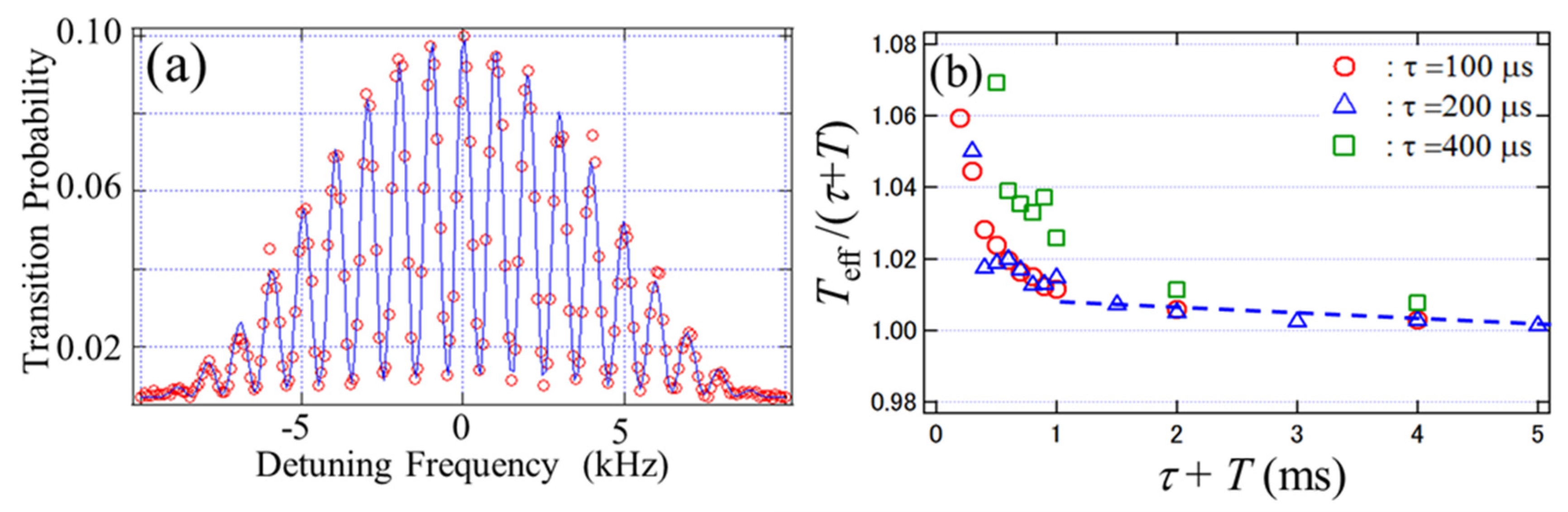
4.3. Ramsey-Type Frequency Standard

We apply the present formula to evaluate the Ramsey atomic frequency standard, where atoms are irradiated by two radio-frequency pulses separated by time T in a homogeneous weak magnetic field. During time T, the atoms are affected by the magnetic field and also by the blackbody radiation from the surrounding environment or stray rf fields. These cause a phase shift and fluctuation due to the scalar Aharonov–Bohm phase, in addition to a frequency shift at the interaction. In the Ramsey frequency standard, the frequency of the applied rf field is stabilized to the frequency at which the transition probability becomes maximum. The frequency is searched for by use of a derivative technique of the transition probability. Under a time-varying potential V(t), the phase at the resonance frequency of the interaction shifts from zero to

$$\phi =\frac{V_1+V_2}{2\hslash }T-\frac{1}{\hslash }{\displaystyle {\int }_{\tau /2}^{\tau /2+T}V(t)dt}$$

(10)

Here, we assumed $\left|\phi \right|\le 2\pi$. As a result, the frequency with the maximum transition probability is

$${\nu }_{\mathrm{L}}={\nu }_0+(V_1+V_2)/(2h)-\phi /\left\{2\pi (\tau +1)\right\}={\nu }_0+\frac{(V_1+V_2)\tau }{2h(\tau +T)}+\frac{1}{h(\tau +T)}{\displaystyle {\int }_{\tau /2}^{\tau /2+T}V(t)dt}$$

(11)

This means that the frequency of the Ramsey frequency standard shifts from the resonance frequency under the zero potential by the integral of the potential with respect to t during the interrogation time divided by h. Therefore, during the interrogation time, all potentials must be measured as a function of time to compensate them. In particular, the strength of the quantization magnetic field must be measured during the interrogation time, because the compensation of the second-order Zeeman effect is relatively larger than those of other potentials.

In a Ramsey atom interferometer—except during the interaction between the two rf pulses—there is no rf field during the interrogation zone. If the AC Stark frequency shift under rf pulses is ν^ac, the phase shift at the frequency of ν₀ + ν^ac is 2πν^acT, according to the first term on the right side of Equation (10). Therefore, the stabilized frequency reverts to the resonance frequency when there is no rf field. In a Ramsey atom interferometer using two-photon Raman pulses, this shift is commonly observed without cancellation of the AC Stark shift [12]. However, in a Cs atomic fountain clock [6], the shift will be negligibly small because the AC Stark shift is too small to detect [17].

5. Conclusions

Using a Ramsey atom interferometer with the two-photon Raman pulses having a duration of τ, which are separated by time T, under a time-varying magnetic field B, the scalar Aharonov–Bohm effect due to the second-order Zeeman potential V(t) was examined experimentally. The effective separation time T_eff that determines the Ramsey fringe cycle is τ + T—namely, the time from the center of the first pulse to that of the second pulse, provided that τ is smaller than T/10. The resonance frequency, which corresponds to the center frequency of the envelope curve of the transition probability, is given by the mean of V₁/h and V₂/h, where V₁ and V₂ are the potentials at the centers of the first and the second pulses, respectively. It was deduced that the phase of the Ramsey fringes at the resonance frequency shifts by

$$\phi =\frac{V_1+V_2}{2\hslash }T-\frac{1}{\hslash }{\displaystyle {\int }_{\tau /2}^{\tau /2+T}V(t)dt}$$

The Ramsey resonance is a superior method of realizing not only the present Cs primary frequency standard but also a future frequency standard with ultimate accuracy, such as a single-ion trap or optical lattice clock. Then, using the formulas derived in this paper, we will be able to accurately evaluate the frequency shift or phase shift due to the scalar Aharonov–Bohm effect for time-varying potentials during a longer interrogation time.

References

1. Ramsey, N.F. A Molecular beam resonance method with separated oscillating fields. Phys. Rev. 1950, 78, 695–698. [Google Scholar] [CrossRef]
2. Bordé, C.J. Atomic interferometry with internal state labelling. Phys. Lett. A 1989, 140, 10–12. [Google Scholar] [CrossRef]
3. Cronin, A.D.; Schmiedmayer, J.; Pritchard, D.E. Optics and interferometry with atoms and molecules. Rev. Mod. Phys. 2009, 81, 1051–1130. [Google Scholar] [CrossRef]
4. Riehle, F.; Kisters, T.; Witte, A.; Helmcke, J.; Bordé, C.J. Optical Ramsey spectroscopy in a rotating frame: Sagnac effect in a matter-wave interferometer. Phys. Rev. Lett. 1991, 67, 177–180. [Google Scholar] [CrossRef] [PubMed]
5. Hudson, J.J.; Kara, D.M.; Smallman, I.J.; Sauer, B.E.; Turbutt, M.R.; Hinds, E.A. Improved measurement of the shape of the electron. Nature 2011, 473, 493–496. [Google Scholar] [CrossRef] [PubMed]
6. Heavner, T.P.; Jefferts, S.R.; Donley, E.A.; Shirley, J.H.; Parker, T.E. NIST-F1: Recent improvements and accuracy evaluations. Metrologia 2005, 42, 411–422. [Google Scholar] [CrossRef]
7. Aharonov, Y.; Bohm, D. Significance of electromagnetic potentials in the quantum theory. Phys. Rev. 1959, 115, 485–490. [Google Scholar] [CrossRef]
8. Allman, B.E.; Cimmino, A.; Opat, G.I.; Klein, A.G.; Kaiser, H.; Werner, S.A. Scalar Aharonov-Bohm experiment with neutrons. Phys. Rev. Lett. 1992, 68, 2409–2412. [Google Scholar] [CrossRef] [PubMed]
9. NicChormaic, S.; Miniatura, C.; Gorceix, O.; Lesengo, B.V.; Robert, J.; Feron, S.; Leorent, V.; Reinhardt, J.; Baudon, J.; Rubin, K. Atomic Stern-Gerlach interferences with time-dependent magnetic fields. Phys. Rev. Lett. 1994, 72, 1–4. [Google Scholar] [CrossRef] [PubMed]
10. Shinohara, K.; Aoki, T.; Morinaga, A. Scalar Aharonov–Bohm effect for ultracold atoms. Phys. Rev. A 2002, 66, 042106. [Google Scholar] [CrossRef]
11. Aoki, T.; Yasuhara, M.; Morinaga, A. Atomic multiple-wave interferometer phase-shifted by the scalar Aharonov–Bohm effect. Phys. Rev. A 2003, 67, 053602. [Google Scholar] [CrossRef]
12. Numazaki, K.; Imai, H.; Morinaga, A. Measurement of the second-order Zeeman effect on the sodium clock transition in the weak-magnetic-field region using the scalar Aharonov–Bohm phase. Phys. Rev. A 2010, 81, 032124. [Google Scholar] [CrossRef]
13. Riehle, F. Frequency Standards, 1st ed.; Wiley-VCH: Weinheim, Germany, 2004; pp. 192–202. [Google Scholar]
14. Moler, K.; Weiss, D.S.; Kasevich, M.; Chu, S. Theoretical analysis of velocity-selective Raman transitions. Phys. Rev. A 1992, 45, 342–348. [Google Scholar] [CrossRef] [PubMed]
15. Nakamura, K.; Murakami, M.; Morinaga, A. Dephasing in sodium Ramsey interferometry under a weak inhomogeneous magnetic field. J. Phys. B 2015, 48, 075001. [Google Scholar] [CrossRef]
16. Tanaka, H.; Imai, H.; Furuta, K.; Kato, Y.; Tashiro, S.; Abe, M.; Tajima, R. Dual magneto-optical trap of sodium atoms in ground hyperfine F = 1 and F = 2 states. Jpn. J. Appl. Phys. 2007, 46, L492–L494. [Google Scholar] [CrossRef]
17. Holloway, J.H.; Racey, R.F. Factors which limit the accuracy of cesium atomic beam frequency standards. In Proceedings of the International Conference on Chronometry, Lausanne, Switzerland, 8–12 June 1964; p. 317.
Figure 1. Ramsey atom interferometer under time-varying potential V(t).
Atoms 04 00023 g001
Figure 2. (a) A partial sodium energy-level scheme and two-photon Raman transition; (b) Experimental set-up. B: quantized magnetic field.
Atoms 04 00023 g002
Figure 3. (a) Ramsey fringes. τ = 100 μs, T = 900 μs; (b) Teff versus τ + T for different τ.
Atoms 04 00023 g003
Figure 4. (a) Three Ramsey fringes in the center of the envelope for two different potentials; (b) Phase shift for two potentials (i) and (ii).
Atoms 04 00023 g004
Figure 5. (a) Three time-varying potentials; (b) Phase shift on resonance for three potentials.
Atoms 04 00023 g005