
Positron-Hydrogen Scattering, Annihilation, and Positronium Formation

Heliophysics Science Division, NASA/Goddard Space Flight Center, Greenbelt, MD 20771, USA
Atoms 2016, 4(4), 27; https://doi.org/10.3390/atoms4040027
Submission received: 14 September 2016
/
Revised: 19 October 2016
/
Accepted: 26 October 2016
/
Published: 4 November 2016
(This article belongs to the Special Issue Positron Scattering and Annihilation with Atoms and Molecules including Emerging New Resonances and their Applications in other Systems)
Abstract
:In previous papers (Bhatia A.K. 2007, 2012) a hybrid theory for the scattering of electrons from a hydrogenic system was developed and applied to calculate scattering phase shifts, Feshbach resonances, and photoabsorption processes. This approach is now being applied to the scattering of positrons from hydrogen atoms. Very accurate phase shifts, using the Feshbach projection operator formalism, were calculated previously (Bhatia A.K. et al. 1971 and Bhatia et al. 1974a). The present results, obtained using shorter expansions in the correlation function, along with long-range correlations in the Schrödinger equation, agree very well with the results obtained earlier. The scattering length is also calculated and the present results are compared with the previous results. Annihilation cross-sections, and positronium formation cross-sections, calculated in the distorted-wave approximation, are also presented.
1. Introduction
Scattering by hydrogenic systems has been carried out using various approximations. Among them is the method of polarized orbitals of Temkin (1959) [1], which takes into account the distortion produced in the target by the incident particle in the ansatz for the wave function for the scattering process. However, this method is not variational and does not provide any bounds on the calculated phase shifts. An alternate approach is to introduce separate correlation functions and amalgamate them into the scattering problem via an optical potential in the scattering equation. The most rigorous approach uses the projection operator formalism of Feshbach [2] (1962). This approach was applied to calculate accurate S and P phase shifts for electron-hydrogen and electron-helium ion scattering by Bhatia and Temkin (2001) [3] and Bhatia (2002, 2004, and 2006) [4,5,6]. The phase shifts obtained have a rigorous lower bound to the exact phase shifts. The close-coupling approach also provides rigorous lower bounds, while the Kohn-variational principle, and other methods related to it, do not. As indicated in the formalism of the hybrid theory by Bhatia (2007, 2008) [7,8] it is not necessary to use Feshbach projection operators to calculate the optical potential which replaces the many-particle Schrödinger equation with a single-particle equation. The phase shifts calculated by Bhatia (2007, 2008) [7,8] have rigorous lower bounds. We now apply this approach to the scattering of positrons from hydrogen atoms. There are no nonlocal potentials in the scattering equation for the scattering function, as in the electron scattering, because of the absence of exchange between positrons and electrons. Previously, Feshbach projection operators were used to carry out the positron-hydrogen scattering calculations of Bhatia et al (1971, 1974) [9,10] and the correction due to the effect of the target polarization was applied to the extrapolated variational results. In spite of the fact that this ad hoc correction destroyed the variational bound, the final results obtained by Bhatia et al. (1971, 1974a) [9,10] have been considered accurate and have stood the test of time. We now apply the hybrid theory to positron scattering and the present calculation includes short-range and long-range correlations at the same time, as mentioned above. The details of this formalism have been given in previous publications of Bhatia (2007, 2008) [7,8] and therefore, we briefly describe the method. The wave function is given by:
where the positron coordinate is given by , the electron coordinate by , and the summation over is from 1 to N, the number of terms in the expansion; are unknown coefficients, and is the correlation function. The correlation functions are short-range in nature in and , and are normalized to unity. Their expectation values of these correlation functions are given by Equation (8). In order to include polarization of the target, the effective target function can be written as:
where Z is the nuclear charge. The function is given by:
The target function is given by:
We find that there is a problem in using the projection operators when polarization of the target is included in the target function. According to Feshbach (1962) [2], the projection operators should be idempotent, i.e.,:
In order to satisfy the above conditions, the perturbed wave function given in Equation (2) must be normalized to unity for all and . This is not possible, as indicated by Bransden (1970) [11]. Therefore, we have not used the projection operators in the present calculation as it becomes too difficult to write the optical potential and to satisfy the above conditions in the presence of the polarization of the target.
Another variational approach, also based on perturbation, has been proposed by Drachman (1968) [12]. He writes the wave function in the form:
where:
The correlation function can be written in the above form, where G is the exact adiabatic perturbation including all multipoles. The functions and are determined variationally using , numerically, obtained from the exact analytic form of G, given in elliptical coordinates by Dalgarno and Lynn (1957) [13]. However, retaining the short-range monopole part is unjustified and by suitably suppressing it, the scattering length and the phase shifts comparable to those of Schwartz (1961) [14] have been obtained.
The variation with respect to , as indicated by Bhatia (2007) [7], in the function:
Gives:
where is given by:
and is the expectation value of H:
In Equation (2), is the smooth cutoff function introduced by Shertzer and Temkin (2006) [15]. This term guarantees that for . This function is given by:
This function is unlike the step function, , introduced by Temkin (1959) [1], which equals 1 when , and equals zero otherwise. This step function ensures that the polarization takes place only when the incident particle is outside the target. Now we want the polarization function in Equation (2) to be valid throughout the range, rather than only for > . The angle is the angle between and . It should be pointed out that in Equation (2), there is a plus sign after the target function and not the negative sign, as in the case of the electron scattering. This is due to the fact that the perturbing potential is of the opposite sign to that in the case of the electron:
The positive sign is for positron scattering and the negative sign for electron scattering. The correctness of the sign in Equation (2) can be ascertained from the paper of Temkin and Lamkin (1961) [16]. In Equation (1), L is the angular momentum, is the scattering function, and the function is the correlation function which can be written in terms of generalized “radial” functions, which depend on the radial coordinates and the Euler angles introduced by Bhatia and Temkin (1964) [17]:
For S-wave (i.e., L = 0) = constant in Equation (13) and is taken of Hylleraas form:
where the sum includes all triplets such that l + m + n = ω and ω = 0, 1, 2, 3, 4, and 5. Bhatia et al. (1971) [9] included a term in the above function to take into account virtual positronium formation. This term has not been included here, and we have not used the Feshbach projection operators either, in the present calculations. The scattering equation with the optical potential becomes simpler without the use of the projection operators. The wave function of the scattered positron is determined from:
In Equation (15), H is the Hamiltonian and E is the total energy of the system. We have used Rydberg units throughout . We have H in these units:
where is the kinetic energy of the incident positron and Z is the nuclear charge.
For L = 0, we can write the equation (15) for the scattering function u in the form:
where:
where:
which can be written as:
where:
In Equations (24a) and (24b) the summation over s is understood. Substituting Equations (19)–(24) in Equation (18), we get the equation for the scattering function u(r):
We give the various quantities:
The direct potentials are given by:
and
The various quantities in the above equation are:
The polarizability of the target is obtained from the following expression for r = infinity:
where:
For r -> infinity, x3 has a term:
where 9/(2Z4) is the dipole polarizability of the target with nuclear charge Z.
Here, is the wave function given in Equation (1) without the correlation term. The phase shifts are inferred from the scattering function uL=0 u for r tending to infinity:
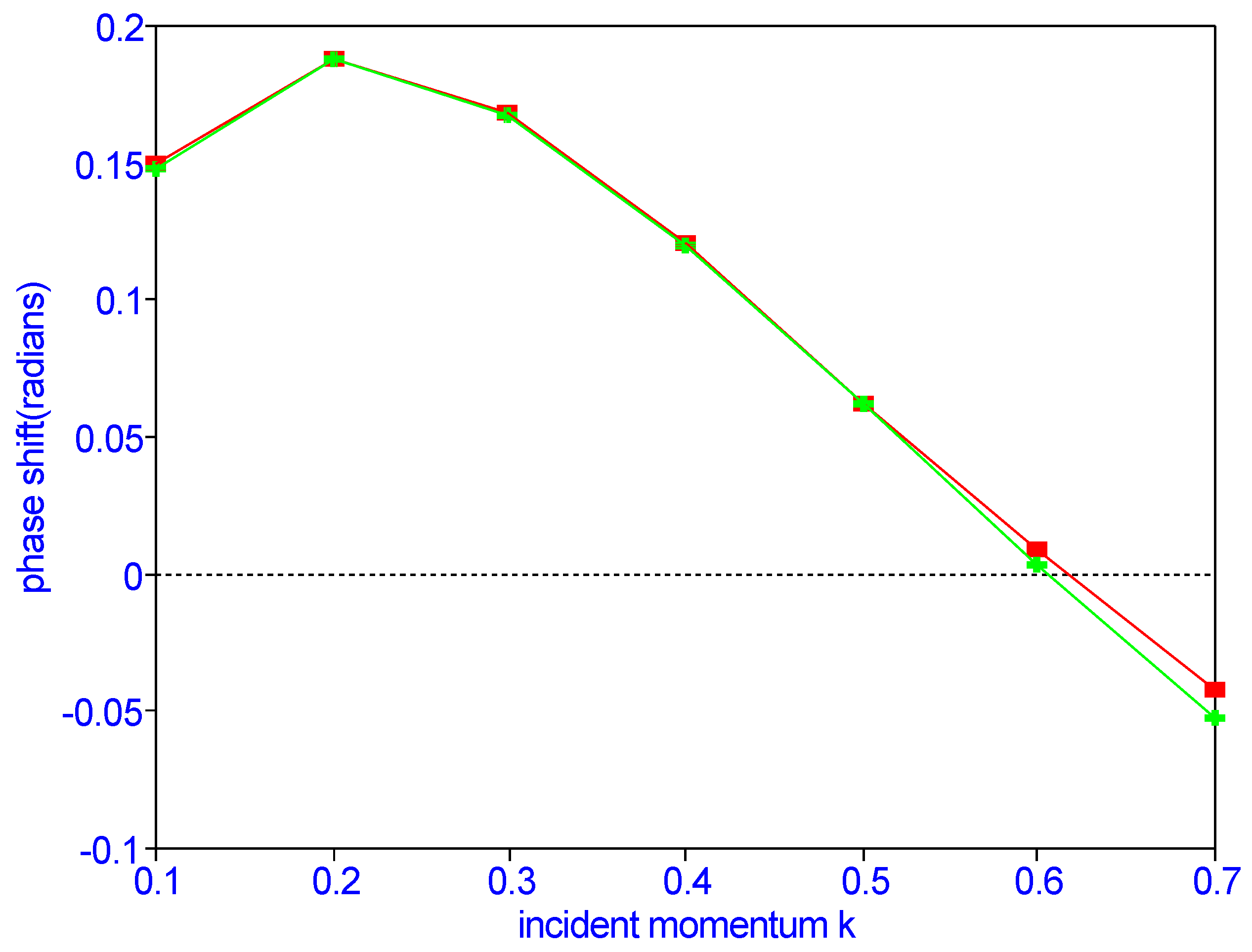
In Table 1, we show the convergence of phase shifts (radians) for k = 0.4 with the number of terms in the correlation function given in Equation (1). By N = 35, the phase shift has converged to at least four significant figures. In Table 2, results, which have not been extrapolated, are given for k = 0.1 to 0.7. The phase shifts obtained for shorter expansions are in good agreement with the previous calculations of Bhatia et al. (1971) [9]. However, the results of Bhatia et al. (1971) have been obtained by extrapolation and by adding the contribution of the long-range potential due to the polarization of the target to the extrapolated results. Their final results do not have any variational bounds anymore. The present and previous results are shown in Figure 1. We also compare the present phase shifts with those obtained by Schwartz (1961) [14] obtained by using the Kohn variational principle, Houston and Drachman (1971) [18], by using the Harris method, Kohn variational calculation of Humberston and Wallace (1972) [19], and Gien (1997) [20], by using the Harris-Nesbet method in Table 2. The 21-state close-coupling approximation phase shifts obtained by Mitroy and Ratnavelu (1995) [21,22,23] are lower than the present results. Mitroy (1995) [21,22,23] has reported a large basis close-coupling calculation of scattering at low energies. The phase shifts of these calculations are lower than the present results given in Table 2. In the most recent publication of Kadyrov and Bray (2016) [24] on the recent progress has given the elastic cross-sections at low positron energies in Figure 6. However, extracting phase shifts from this figure will not be accurate enough for comparison with the present calculations. Phase shifts obtained by Higgins (1990) [25], using intermediate R-matrix theory, are also given in Table 2. The agreement of the results of these calculations is good. However, they are lower than the present results. The phase shifts of Schwartz (1961) [14] are wrong at two incident positron momenta.
The scattering length is given by:
In Table 3 we show the convergence of the scattering length with the number of terms in the correlation function given in Equation (1). Temkin (1961) [26] showed that there is a correction due to the long-range correlations:
The scattering length given in Table 3 for N = 56 has been calculated at R = 1856.470. Only the term contributes significantly in Equation (41). The final result for the scattering length = −2.10158 − 0.002424 = −2.104004 a0. This agrees with the scattering length −2.1036 0.0004 obtained by Houston and Drachman (1971) [18], and with −2.103 0.001 by Humberston and Wallace (1972) [19], using the Kohn variational principle. Another formula obtained by Drachman (2016) [27] using the Calogero method (1967) [28] for a correction due to the long-range correlation is:
This give a = −2.104007a0, which is essentially the result obtained using Equation (41). This result is consistent with the convergence of Schwartz’s calculation (1961) [14] that −2.10 > a > −2.11.
Using the presently calculated scattering length, the cross-section at zero energy is given by . If the experimental results of Zhou et al. (1997) [29] are extrapolated towards zero energy, then their result is found to be too low. The present result for the cross-section should be correct because the scattering length is well established by now, having being previously calculated by Schwartz (1961) [14], Houston and Drachman (1971) [18], and Humberston and Wallace (1972) [19]. Since only S-wave phase shifts have been calculated here, a comparison with the experimental results at higher energies cannot be made.
2. Zeff
In addition to the scattering, there is a possibility of positronium formation and positron annihilation. The cross-section for annihilation of an incoming positron and an atomic electron with the emission of two gamma rays is given by Ferrell (1956) [32]:
where is the fine-structure constant and is the Bohr radius. As the quantity , which measures the overlap of the target electron with the positron, as indicated by DiRienzi and Drachman (2003) [33], approaches Z, the number of electrons for a free positron. For hydrogen:
The normalization of in Equation (1) requires that for :
In Table 4 we present values for Zeff for L = 0 as a function of k below the positronium formation threshold. The present results are compared with the previous results by Bhatia et al. (1974b) [34] and with those obtained by Humberston and Wallace (1972) [19]. The agreement is fairly good. Green and Gribakin (2013) [35], using the diagrammatic many-body theory have calculated phase shifts and Zeff, given in their Figure 7. Their results for Zeff, given in Table 4, could not be read accurately from the figure. Nevertheless, their results appear to be close to those obtained in other calculations. It is found empirically that the value of Zeff at very low energies is proportional to the dipole polarizability α of the hydrogen atom (Osmon, 1965) [36] and can be represented by . The annihilation of positrons with electrons results in two photons at a rate λ, Fraser (1968) [37]:
3. Positronium Formation
Positronium, the bound state of an electron and a positron, was predicted by Mohorovicic (1934) [38] in connection with the spectra of nebulae. Positronium formation takes place when the incident positron captures an electron of the hydrogen atom before the positron and electron annihilate each other:
where Ps is the positronium atom and P is the proton. Experimental determination of the cross-section of positronium formation in various gases have been carried out by Charlton (1985) [39] and Stein et al. (1992) [40]. Experiments on hydrogen atoms have been carried out by Zhou et al. (1997) [29]. R-matrix calculations have been carried out by Chan and Fraser (1973) [41], while coupled-channel calculations have been carried out by Humberston (1982) [42]. Using the distorted-wave approximation, Khan and Ghosh (1983) [43] have carried their calculations using the method of polarized orbitals of Temkin (1959) [1]. The present calculations are similar to those of Khan and Ghosh. However, the scattering functions have been calculated variationally by Bhatia (2007, 2008) [7,8]. The differential cross-section for this rearrangement collision from the ground state is given by:
In the above equation, vi and vPS are the velocities of the incident positron and of positronium in the final state, ki and kPs are the momenta of the incident positron and positronium atom in the final state, and and are the initial and final reduced masses equal to 1/2 and 1, respectively, in Rydberg units. T is the transition matrix which is given by Khan and Ghosh (1983) [43] and Bransden (1965) [44].
where
The ground state wave function of the positronium atom is given by:
The interaction potential in the final state is given by:
In Rydberg units, being used throughout, is equal to 2 and is equal to 1.
We can write:
The first term above involves the target function only and the second terms involve the polarization of the target, as indicated in Equation (2). The integration of these terms can be carried out by using Fourier transforms, given in Khan and Ghosh (1983) [43] and Cheshire (1964) [45], of various terms in the integrand, as indicated in the appendix. We consider L = 0 and the wave function for the initial state is given in Equation (1) without the correlation terms. The differential cross-section is given by:
where T’ is given in the Appendix. The total cross section is given by:
In units, the cross-section is given by:
We have used in Rydberg units. Cross-sections obtained using only , and using for positronium formation at various energies are given in Table 5 and compared with those obtained by Khan and Ghosh (1983) [43]. The first column gives cross-sections without the polarization of the target and their maximum value occurs at = 0.75 while, with polarization, the maximum is at = 0.80. The cross-sections increase considerably when the polarization of the target is taken into account. It is seen that the present results agree with results of Khan and Ghosh (1983) [43] and are also in reasonable agreement with those of Humberston (1982) [42]. The present results are also in reasonable agreement with those of Chan and Fraser (1973) [41] when the second term in Equation (53) is not included. This is rather surprising since polarization is very important in the positron-hydrogen scattering. The present results are also compared with those of Kvitsinsky et al. (1995) [46] who used the Fadeev equations for their calculations. Again, the presently-calculated cross-sections are only at S-wave, and they cannot be compared with the experimental results of Zhou et al. (1997) [29]. Similarly, higher partial waves are required to calculate differential cross-sections.
4. Conclusions
Using the hybrid theory of scattering of Bhatia (2007) [47], we have calculated phase shifts which have lower bounds to exact phase shifts. This calculation, which includes the contribution of the long-range interaction variationally, requires fewer correlation functions compared to the previous calculation of Bhatia et al. (1971) [9]. The scattering length also agrees with previous calculations of Schwartz (1961) [14] and Houston and Drachman (1971) [18]. The scattering functions have been further used to calculate and positronium formation cross-sections in the distorted-wave approximation. The scattering functions obtained using the hybrid theory have been used previously to calculate phase shifts and photoabsorption cross-sections by Bhatia (2004, 2006, and 2008) [5,6,8], giving results agreeing with those obtained using different methods. Equation (25) can be used to calculate bound state energies as well, as indicated by Bhatia and Madan (1973) [48]. It is expected that the present results should be accurate, as well, up to the fourth decimal place.
Acknowledgments
Thanks are extended to R. J. Drachman for many helpful discussions, for a table of Fourier transforms, for bringing to my attention his publication of 1968 on this topic, and for critical reading of the manuscript. I would like to thank Hasi Ray for pointing out the publication of Cheshire (1964) [45] on Fourier transforms during her stay at Goddard in 2015. Calculations were carried out in quadruple precision using the Discover computer of the NASA Center for Computation Science.
Conflicts of Interest
The authors declare no conflict of interest.
Appendix A
The integrals occurring in the calculation are of the form:
and
where
and
The integration of these two integrals can be carried out using the Fourier transforms:
and
The limits of integration are from = 0 to = 1 in Equations (A7) and (A8) are:
The other required integrations in involving powers of and can be obtained by differentiating and with respect to λ and α, respectively, in the Fourier transforms shown in Equations (A6) and (A7).
DiRienzi and Drachman (2003) [33] also used Fourier transforms and contour integration for evaluating integrals occurring in their positronium-helium scattering.
References
- Temkin, A. A Note on the Scattering of Electrons from Atomic Hydrogen. Phys. Rev. 1959, 116, 358. [Google Scholar] [CrossRef]
- Feshbach, H. A unified theory of nuclear reactions. II. Ann. Phys. 1962, 19, 287–313. [Google Scholar] [CrossRef]
- Bhatia, A.K.; Temkin, A. Complex-correlation Kohn T-matrix method of calculating total and elastic cross sections: Electron-hydrogen elastic scattering. Phys. Rev. A 2001, 64, 032709. [Google Scholar] [CrossRef]
- Bhatia, A.K. Electron-He+ elastic scattering. Phys. Rev. A 2002, 66, 064702. [Google Scholar]
- Bhatia, A.K. Electron-hydrogen P-wave elastic scattering. Phys. Rev. A 2004, 69, 032714. [Google Scholar] [CrossRef]
- Bhatia, A.K. Electron-He+ P-wave elastic scattering and photoabsorption in two-electron systems. Phys. Rev. A 2006, 73, 012705. [Google Scholar] [CrossRef]
- Bhatia, A.K. Hybrid theory of electron-hydrogen elastic scattering. Phys. Rev. A 2007, 75, 032713. [Google Scholar] [CrossRef]
- Bhatia, A.K. Applications of the hybrid theory to the scattering of electrons from He+ and Li2+ and resonances in these systems. Phys. Rev. A 2008, 77, 052707. [Google Scholar] [CrossRef]
- Bhatia, A.K.; Temkin, A.; Drachman, R.J.; Eiserike, H. Generalized Hylleraas Calculation of Positron-Hydrogen Scattering. Phys. Rev. A 1971, 3, 1328. [Google Scholar] [CrossRef]
- Bhatia, A.K.; Temkin, A.; Eiserike, H. Rigorous precision p-wave positron-hydrogen scattering calculation. Phys. Rev. A 1974, 9, 219. [Google Scholar] [CrossRef]
- Bransden, B.H. Atomic Collision Theory; W.A. Benjamin Inc.: New York, NY, USA, 1970. [Google Scholar]
- Drachman, R.J. Variational Bounds in Positron-Atom Scattering. Phys. Rev. 1968, 173, 190. [Google Scholar] [CrossRef]
- Dalgarno, A.; Lynn, N. An Exact Calculation of Second Order Long Range Forces. Proc. Phys. Soc. A 1957, 70, 223. [Google Scholar] [CrossRef]
- Schwartz, C. Electron Scattering from Hydrogen. Phys. Rev. 1961, 124, 1468. [Google Scholar] [CrossRef]
- Shertzer, J.; Temkin, A. Direct calculation of the scattering amplitude without partial-wave analysis. III. Inclusion of correlation effects. Phys. Rev. A 2006, 74, 052701. [Google Scholar] [CrossRef]
- Temkin, A.; Lamkin, J.C. Application of the Method of Polarized Orbitals to the Scattering of Electrons from Hydrogen. Phys. Rev. 1961, 121, 788. [Google Scholar] [CrossRef]
- Bhatia, A.K.; Temkin, A. Symmetric Euler-Angle Decomposition of the Two-Electron Fixed-Nucleus Problem. Rev. Mod. Phys. 1964, 36, 1050. [Google Scholar] [CrossRef]
- Houston, S.K.; Drachman, R.J. Positron-Atom Scattering by the Kohn and Harris Methods. Phys. Rev. A 1971, 3, 1335. [Google Scholar] [CrossRef]
- Humberston, J.W.; Wallace, J.B.G. The elastic scattering of positrons by atomic hydrogen. J. Phys. B 1972, 5, 1138. [Google Scholar] [CrossRef]
- Gien, T.T. Coupled-state calculations of positron-hydrogen scattering. Phys. Rev. A 1997, 56, 1332. [Google Scholar] [CrossRef]
- Mitroy, J.; Ratnavalu, K. The positron-hydrogen system at low energies. J. Phys. B 1995, 28, 287. [Google Scholar] [CrossRef]
- Mitroy, J. Large Basis Calculation of Positron? Hydrogen Scattering at Low Energies. Aust. J. Phys. 1995, 48, 645–676. [Google Scholar] [CrossRef]
- Mitroy, J. Positronium-Proton Scattering at Low Energies. Aust. J. Phys. 1995, 48, 893–906. [Google Scholar] [CrossRef]
- Kadyrov, A.S.; Bray, I. Recent Progress in the Description of Positron Scattering from Atoms Using the Convergent Close-Coupling Theory. 2016; arXiv:1609.04082. [Google Scholar]
- Higgin, K.; Burke, P.G.; Walters, H.R. Positron scattering by atomic hydrogen at intermediate energies. J. Phys. B 1990, 23, 1345–1357. [Google Scholar] [CrossRef]
- Temkin, A. Polarization and the Triplet Electron-Hydrogen Scattering Length. Phys. Rev. Lett. 1961, 6, 354. [Google Scholar] [CrossRef]
- Drachman, R.J.; (Greenbelt, Maryland, USA). Private communication, 2016.
- Calogero, F. Variable Approach to Potential Scattering; Academic Press: New York, NY, USA, 1971. [Google Scholar]
- Zhou, S.; Li, H.; Kaupppila, W.E.; Kwan, C.K.; Stein, T.S. Measurements of total and positronium formation cross sections for positrons and electrons scattered by hydrogen atoms and molecules. Phys. Rev. A 1997, 55, 361. [Google Scholar] [CrossRef]
- Drachman, R.J. Electron Atomic Collisions. Proc. Int. Conf. Phys. 1971, 277. [Google Scholar]
- Bhatia, A.K. Positron Interactions with Atoms and Ions. J. At. Mol. Condens. Nano Phys. 2014, 1, 45. [Google Scholar]
- Ferrall, R.A. Theory of Positron Annihilation in Solids. Rev. Mod. Phys. 1956, 28, 308. [Google Scholar] [CrossRef]
- DiRienzi, J.; Drachman, R.J. Re-examination of a simplified model for positronium–helium scattering. J. Phys. B 2003, 36, 2409. [Google Scholar] [CrossRef]
- Bhatia, A.K.; Drachman, R.J.; Temkin, A. Annihilation during positron-hydrogen collisions. Phys. Rev. A 1974, 9, 223. [Google Scholar] [CrossRef]
- Green, D.G.; Gribakin, G.F. Positron scattering and annihilation in hydrogen like ions. Phys. Rev. A 2013, 88, 032708. [Google Scholar] [CrossRef]
- Osmon, P.E. Positron Lifetime Spectra in Molecular Gases. Phys. Rev. 1965, 140, A8. [Google Scholar] [CrossRef]
- Fraser, P.A. Positrons and Positronium in Gases. Adv. At. Mol. Phys. 1968, 4, 63–107. [Google Scholar]
- Mohorovicic, S. Möglichkeit neuer Elemente und ihre Bedeutung für die Astrophysik. Astron. Nachr. 1934, 253, 93. [Google Scholar] [CrossRef]
- Charlton, M. Experimental studies of positrons scattering in gases. Rep. Prog. Phys. 1985, 48, 737. [Google Scholar] [CrossRef]
- Stein, T.S.; Kauppila, W.E.; Kwan, C.K.; Parikh, S.P.; Zhou, S. Measurements of positronium formation cross sections for positron-ar and-K scattering. Hyperfine Interact. 1992, 73, 53–63. [Google Scholar]
- Chan, Y.F.; Fraser, P.A. S-wave positron scattering by hydrogen atoms. J. Phys. B 1973, 6, 2504. [Google Scholar] [CrossRef]
- Humberston, J.W. Positronium formation in s-wave positron–hydrogen scattering. Can. J. Phys. 1982, 60, 591–596. [Google Scholar] [CrossRef]
- Khan, A.; Ghosh, A.S. Positronium formation in positron-hydrogen scattering. Phys. Rev. A 1983, 27, 1904. [Google Scholar] [CrossRef]
- Bransden, B.H. Atomic Rearrangement Collisions. Adv. At. Mol. Phys. 1965, 1, 85–148. [Google Scholar]
- Cheshire, I.M. Positronium formation by fast positrons in atomic hydrogen. Proc. Phys. Soc. 1964, 83, 227. [Google Scholar] [CrossRef]
- Kvitsinsky, A.A.; Wu, A.; Hu, C.-Y. Scattering of electrons and positrons on hydrogen using the Faddeev equations. J. Phys. B 1995, 28, 275. [Google Scholar] [CrossRef]
- Bhatia, A.K. Hybrid theory of P-wave electron-hydrogen elastic scattering. Phys. Rev. A 2012, 85, 052708. [Google Scholar] [CrossRef]
- Bhatia, A.K.; Madan, R.N. S-Matrix Method for the Numerical Determination of Bound States. Phys. Rev. A 1973, 7, 523. [Google Scholar] [CrossRef]
Figure 1.
(Color online) The upper curve represents the present results, while the lower curve represents results obtained by Bhatia et al. (1971) [9].
Figure 1.
(Color online) The upper curve represents the present results, while the lower curve represents results obtained by Bhatia et al. (1971) [9].


Table 1.
Convergence of phase shifts (radians) for e+-H scattering with respect to the number of correlation terms N for k = 0.4.
| N | |||
|---|---|---|---|
| 10 | 0.56 | 0.90 | 0.09649 |
| 20 | 0.56 | 0.90 | 0.11619 |
| 35 | 0.60 | 0.91 | 0.11976 |
| 56 | 0.72 | 0.83 | 0.12083 |
Table 2.
Phase shifts ( radians) e+-H scattering for various k and comparison with previous calculations.
| K | N | Present | A | B | C | D | E | F | G |
|---|---|---|---|---|---|---|---|---|---|
| 0.1 | 35 | 0.14918 | 0.1483 | 0.151 | 0.149 | 0.148 | 0.1482 | 0.142 | 0.1404 |
| 0.2 | 35 | 0.18803 | 0.1877 | 0.188 | 0.189 | 0.187 | 0.1875 | 0.182 | 0.1767 |
| 0.3 | 35 | 0.16831 | 0.1677 | 0.168 | 0.169 | 0.167 | 0.1671 | 0.159 | 0.1558 |
| 0.4 | 56 | 0.12083 | 0.1201 | 0.120 | 0.123 | 0.119 | 0.1196 | 0.111 | 0.1105 |
| 0.5 | 20 | 0.06278 | 0.0624 | 0.062 | 0.065 | 0.062 | 0.0621 | 0.055 | 0.0536 |
| 0.6 | 20 | 0.00903 | 0.0039 | 0.007 | 0.008 | 0.003 | 0.0033 | −0.002 | −0.004 |
| 0.7 | 20 | −0.04253 | −0.0512 | −0.054 | −0.049 | … | −0.0520 | −0.0588 |
Table 3.
Convergence of the scattering length for e+-H scattering with respect to the number of correlation terms N.
| N | A | ||
|---|---|---|---|
| 10 | 0.56 | 0.90 | −1.86341 |
| 20 | 0.56 | 0.82 | −2.05266 |
| 35 | 0.56 | 0.84 | −2.10074 |
| 56 | 0.52 | 0.84 | −2.10158 |
Table 4.
Zeff (0) as a function of the incident positron momentum k, obtained in this calculation and compared with previous calculations.
| k | A | B | C | D |
|---|---|---|---|---|
| 0.1 | 8.092 | 7.363 | 7.5 | 7.5 |
| 0.2 | 5.357 | 5.538 | 5.7 | 5.5 |
| 0.3 | 4.264 | 4.184 | 4.3 | 4.1 |
| 0.4 | 3.370 | 3.327 | 3.3 | 3.5 |
| 0.5 | 2.424 | 2.730 | 2.7 | 3.0 |
| 0.6 | 2.249 | 2.279 | 2.3 | 2.8 |
| 0.7 | 2.069 | 1.950 | … | 2.2 |
Table 5.
Comparison of the present results for the positronium formation cross-section ( ) with those obtained in other calculations.
| A | B | C | D | E | |
|---|---|---|---|---|---|
| 0.5041 | 0.0010053 | 0.0066228 | 0.009037 | 0.0041 | 0.0038 |
| 0.5476 | 0.0025753 | 0.018783 | ... | … | ... |
| 0.5625 | 0.0026829 | 0.020249 | 0.024795 | 0.0044 | 0.0041 |
| 0.64 | 0.0025604 | 0.022566 | 0.0248 | 0.0049 | 0.0047 |
| 0.6724 | 0.002412 | 0.022350 | ... | … | ... |
| 0.7225 | 0.0021366 | 0.021456 | 0.021164 | 0.0058 | ... |
| 0.75 | 0.0020034 | 0.020835 | 0.019707 | ... | ... |
| 0.81 | 0.0017211 | 0.019256 | ... | ... | ... |
| 0.9025 | 0.0013698 | 0.016760 | ... | ... | ... |
| 1.00 | 0.0010916 | 0.014327 | ... | ... | ... |
© 2016 by the author; licensee MDPI, Basel, Switzerland. This article is an open access article distributed under the terms and conditions of the Creative Commons Attribution (CC-BY) license (http://creativecommons.org/licenses/by/4.0/).
Share and Cite
MDPI and ACS Style
Bhatia, A.K. Positron-Hydrogen Scattering, Annihilation, and Positronium Formation. Atoms 2016, 4, 27. https://doi.org/10.3390/atoms4040027
AMA Style
Bhatia AK. Positron-Hydrogen Scattering, Annihilation, and Positronium Formation. Atoms. 2016; 4(4):27. https://doi.org/10.3390/atoms4040027
Chicago/Turabian StyleBhatia, Anand K. 2016. "Positron-Hydrogen Scattering, Annihilation, and Positronium Formation" Atoms 4, no. 4: 27. https://doi.org/10.3390/atoms4040027
Note that from the first issue of 2016, this journal uses article numbers instead of page numbers. See further details here.