
The Role of the Hyperfine Structure for the Determination of Improved Level Energies of Ta II, Pr II and La II

Abstract
:1. Introduction
2. Ta II
3. Pr II
4. La II
5. Conclusions
Acknowledgments
Conflicts of Interest
Appendix

| Line | Upper level | Lower Level | References to Cols. | |||||||||||||
|---|---|---|---|---|---|---|---|---|---|---|---|---|---|---|---|---|
| Fig. No. | Sp. | Wavelength (Å) | SNR | Energy (cm−1) | J | P | A (MHz) | B(MHz) | Energy (cm−1) | J | P | A (MHz) | B(MHz) | 5,10 | 8,9 | 13,14 |
| 1 | 2 | 3 | 4 | 5 | 6 | 7 | 8 | 9 | 10 | 11 | 12 | 13 | 14 | 15 | 16 | 17 |
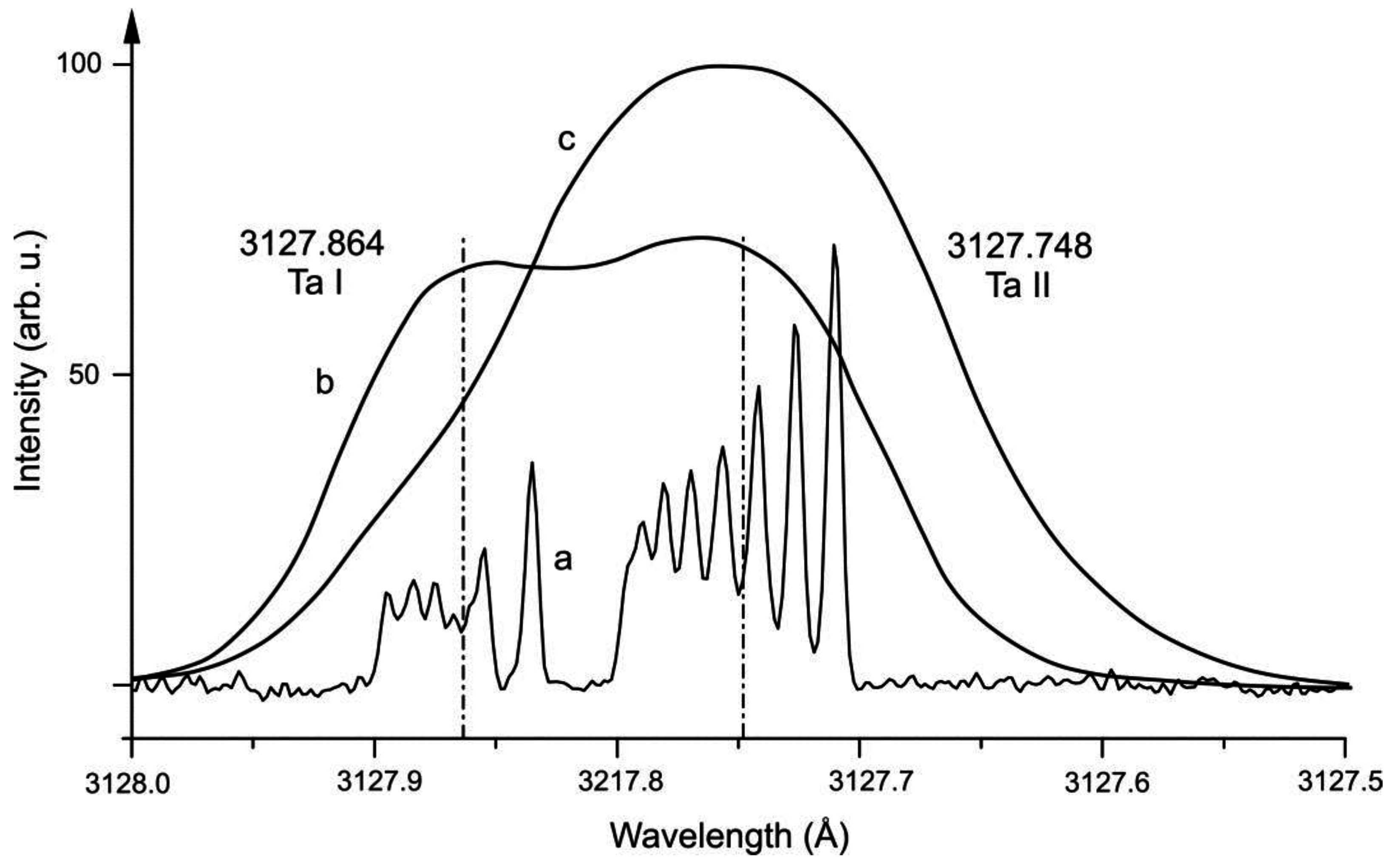
| 1 | Ta II | 3127.748 | 86 | 41708.994 | 5 | o | 914(5) | 350(100) | 9746.376 | 4 | e | 303(10) | 1680(300) | [25] | [25] | [25] |
| 1 | Ta I | 3127.864 | 30 | 31961.442 | 5/2 | o | 1243(3) | 740(10) | 0 | 3/2 | e | 509.084(1) | −1012.238(8) | [18] | tw | [55] |
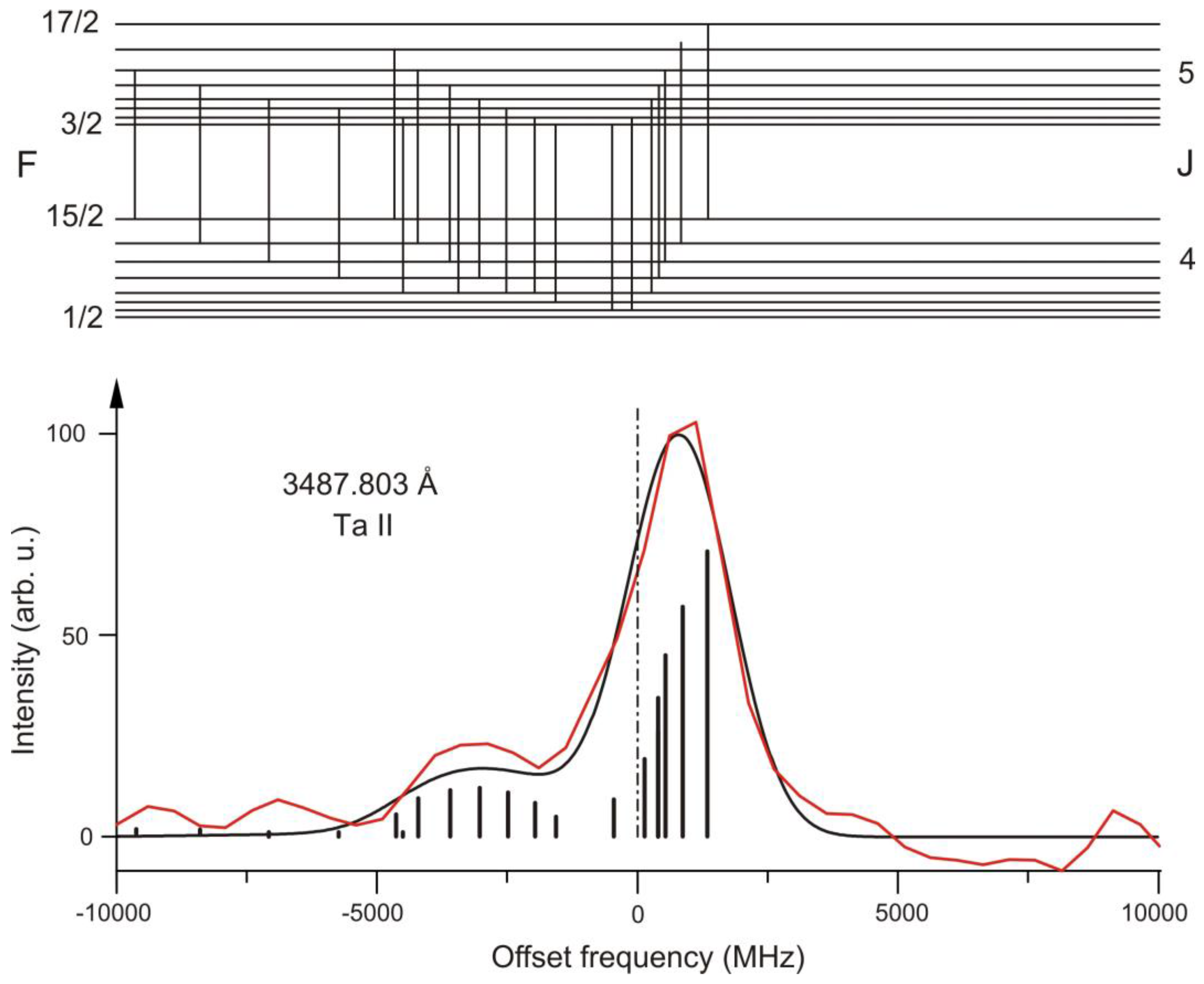
| 2 | Ta II | 3487.803 | 21 | 54048.682 | 5 | o | 650(10) | 1200(200) | 25385.546 | 4 | e | 730(20) | 0(200) | [25] | [25] | [25] |
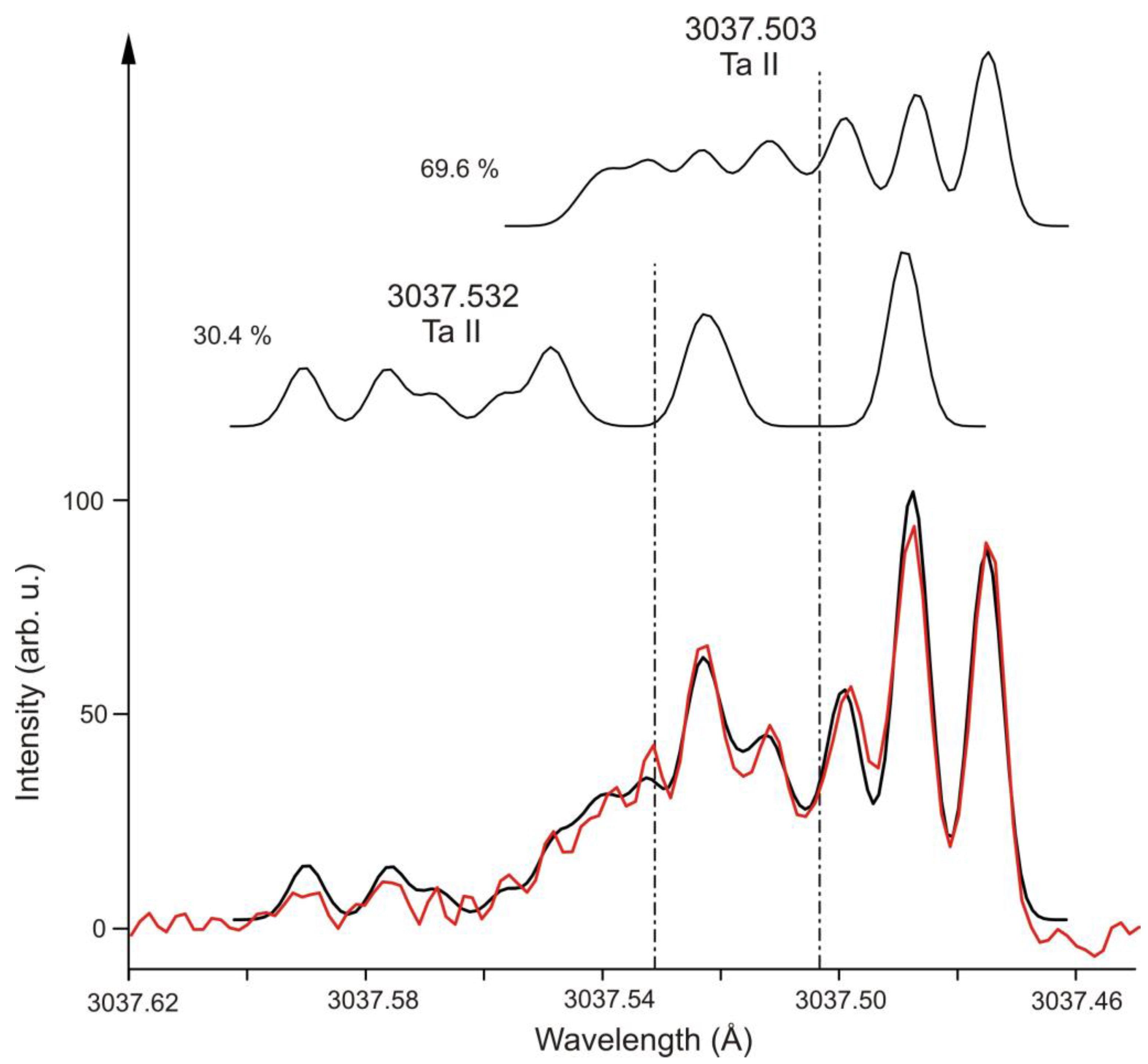
| 3 | Ta II | 3037.503 | 39 | 39743.636 | 4 | o | 955(5) | −1200(100) | 6831.437 | 3 | e | 360(10) | 970(200) | [25] | [25] | [25] |
| 3 | Ta II | 3037.532 | 17 | 46387.287 | 2 | o | 1802(15) | −130(50) | 13475.416 | 1 | e | −480(4) | 724(20) | [25] | [25] | [21] |
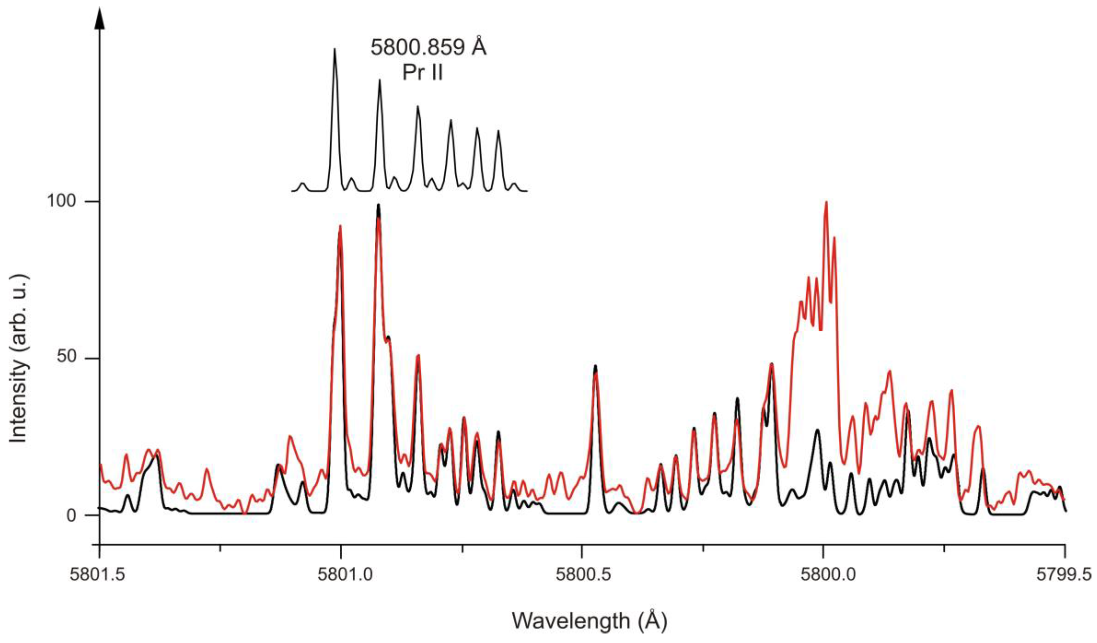
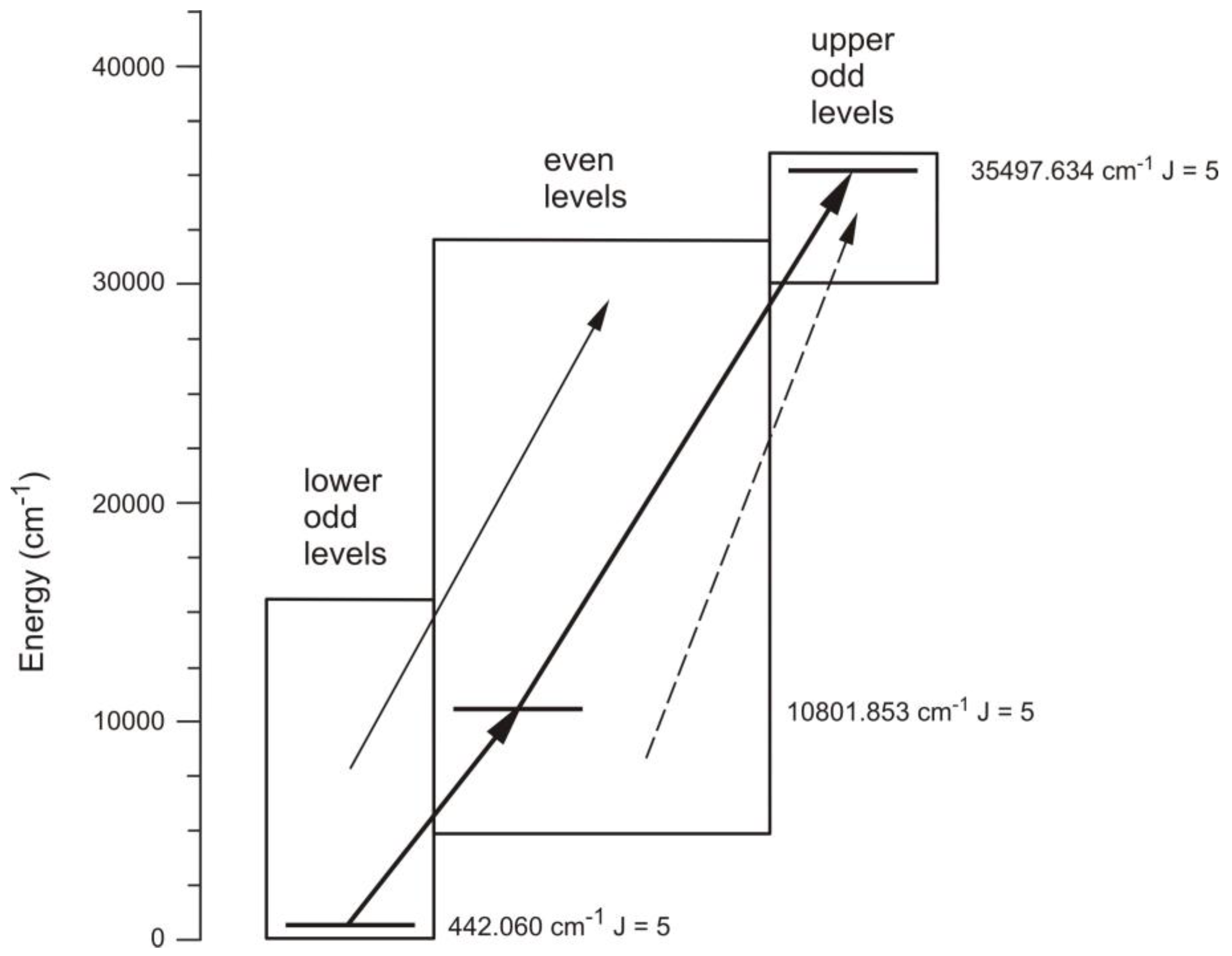
| 5 | Pr II | 5800.859 | 16 | 17676.112 | 5 | e | 805 | - | 442.060 | 5 | o | 1910.3(21) | - | [40] | [34] | [42] |
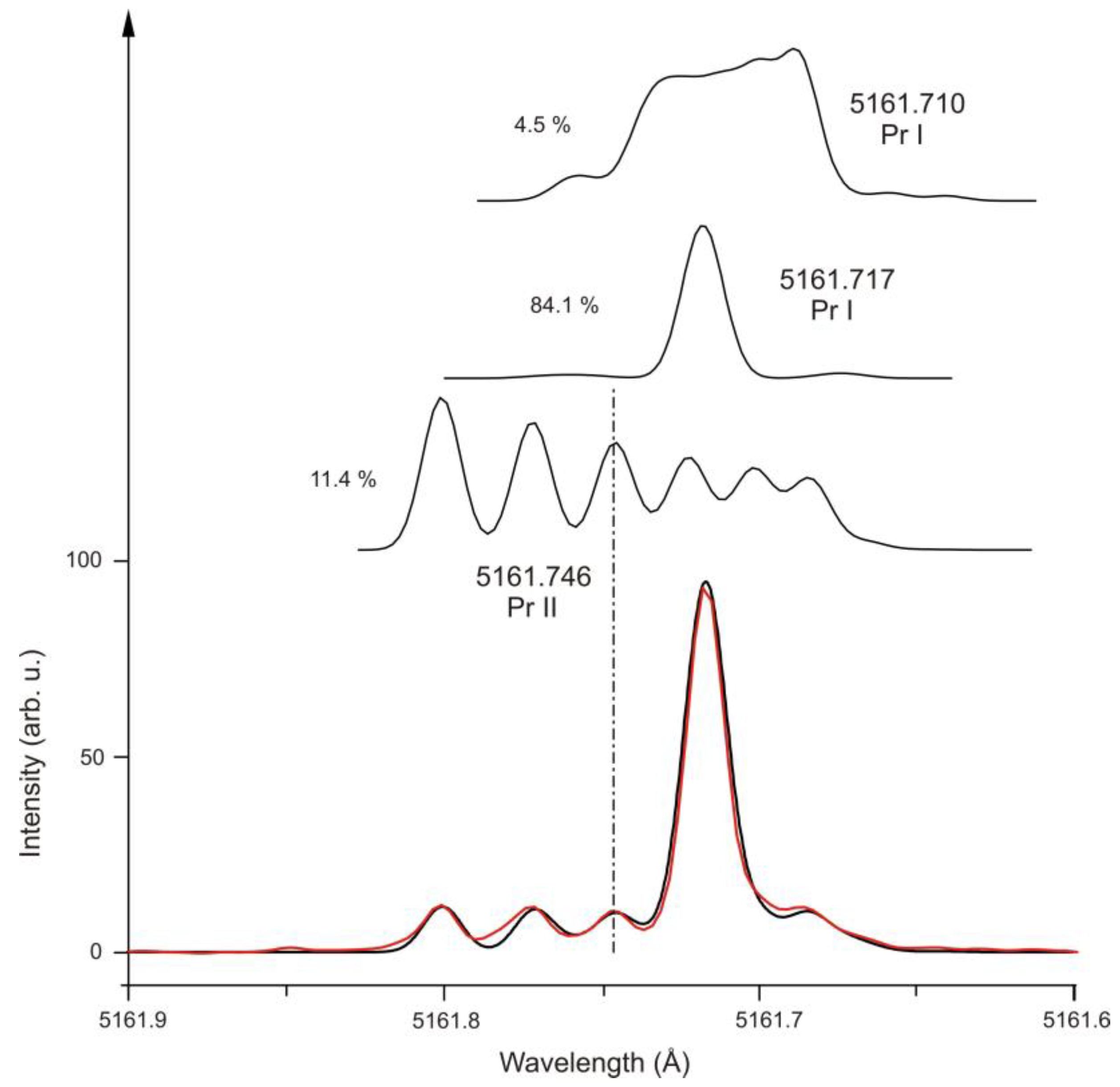
| 7 | Pr I | 5161.710 | 15 | 33932.700 | 13/2 | o | 737(1) | - | 14564.673 | 13/2 | e | 577(2) | - | [38] | [38] | [37] |
| 7 | Pr I | 5161.717 | 280 | 29899.954 | 17/2 | o | 529(1) | - | 10531.951 | 17/2 | e | 546(3) | - | [38] | [38] | [38] |
| 7 | Pr II | 5161.746 | 38 | 23261.402 | 5 | e | 581.9(3) | −19(5) | 3893.46 | 6 | o | 902.1 | - | [40] | [41] | [34] |
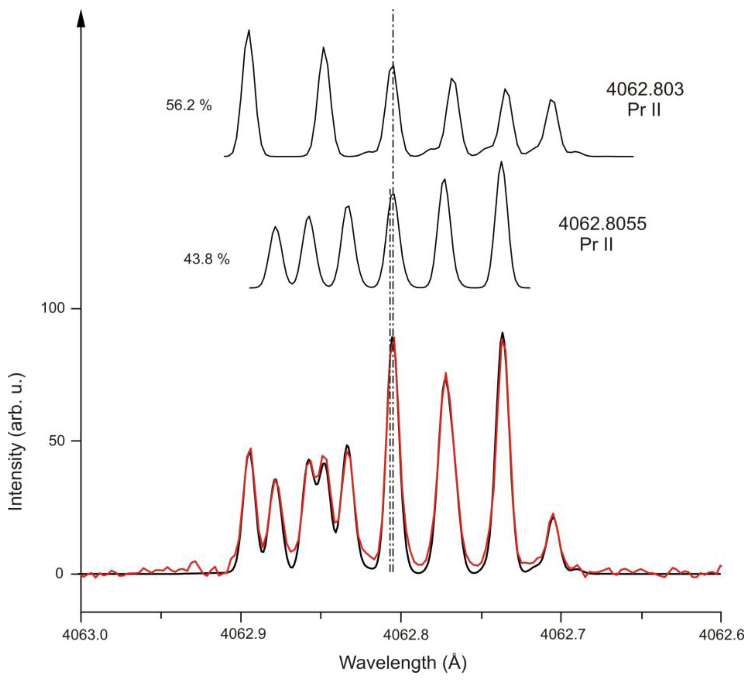
| 8 | Pr II | 4062.803 | 55 | 28009.828 | 7 | e | 556.5(7) | −34(25) | 3403.226 | 6 | o | −146.5(4) | - | [40] | [41] | [42] |
| 8 | Pr II | 4062.8055 | 34 | 27604.990 | 6 | e | 597.0(5) | 1(32) | 2998.412 | 7 | o | 1435.2(16) | - | [40] | [41] | [42] |
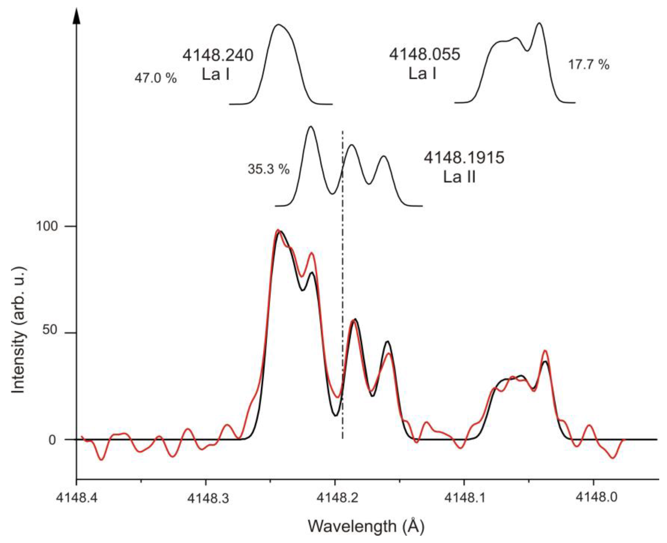
| 9 | La I | 4148.055 | 6 | 33820.316 | 1/2 | o | −232.7(60) | - | 9719.429 | 3/2 | e | −655.138 | −33.249 | tw | [56] | [57] |
| 9 | La II | 4148.1915 | 12 | 51524.005 | 2 | e | −220(3) | - | 27423.911 | 1 | o | 886.9(15) | −18.9(48) | [53] | [53] | [49] |
| 9 | La I | 4148.240 | 16 | 38903.885 | 5/2 | e | 181(3) | - | 14804.067 | 5/2 | o | 335.01(74 ) | 23.64(95) | [58] | [58] | [59] |
| 10 | La II | 4151.957 | 24 | 25973.360 | 1 | o | 547.3(30) | 27(7) | 1895.128 | 1 | e | −1128.1(0.9) | 49.8(65) | [53] | [52] | [45] |
References
- Windholz, L.; Gamper, B.; Binder, T. Variation of the observed widths of La I lines with the energy of the upper excited levels, demonstrated on previously unknown energy levels. Spectr. Anal. Rev. 2016, 4, 23–40. [Google Scholar] [CrossRef]
- Siddiqui, I.; Khan, S.; Windholz, L. Experimental investigation of the hyperfine spectra of Pr I—Lines: Discovery of new fine structure energy levels of Pr I using LIF spectroscopy with medium angular momentum quantum number between 7/2 and 13/2. Eur. Phys. J. D 2016, 70, 44. [Google Scholar] [CrossRef]
- Głowacki, P.; Uddin, Z.; Guthöhrlein, G.H.; Windholz, L.; Dembczyński, J. A study of the hyperfine structure of Ta I lines based on Fourier transform spectra and laser-induced fluorescence. Phys. Scr. 2009, 80, 025301. [Google Scholar] [CrossRef]
- Stone, N.J. Table of nuclear magnetic dipole and electric quadrupole moments. Atom. Data Nucl. Data 2003, 90, 75–176. [Google Scholar] [CrossRef]
- Moore, C.E. Atomic Energy Levels, Vol. III; Circular of the National Bureau of Standards 467; U.S. Government Printing Office: Washington, DC, USA, 1958.
- Martin, W.C.; Zalubas, R.; Hagan, L. Atomic Energy Levels—The Rare Earth Elements; National Bureau of Standards: Washington, DC, USA, 1978.
- Windholz, L. Finding of previously unknown energy levels using Fourier-transform and laser spectroscopy. Phys. Scr. 2016, 91, 114003. [Google Scholar] [CrossRef]
- Messnarz, D.; Jaritz, N.; Arcimowicz, B.; Zilio, V.O.; Engleman, R., Jr.; Pickering, J.C.; Jäger, H.; Guthöhrlein, G.H.; Windholz, L. Investigation of the hyperfine structure of Ta I lines (VII). Phys. Scr. 2003, 68, 170–191. [Google Scholar] [CrossRef]
- Gamper, B.; Uddin, Z.; Jagangir, M.; Allard, O.; Knöckel, H.; Tiemann, E.; Windholz, L. Investigation of the hyperfine structure of Pr I and Pr II lines based on highly resolved Fourier transform spectra. J. Phys. B At. Mol. Opt. 2011, 44, 045003. [Google Scholar] [CrossRef]
- Güzelçimen, F.; Gö, B.; Tamanis, M.; Kruzins, A.; Ferber, R.; Windholz, L.; Kröger, S. High-resolution Fourier transform spectroscopy of lanthanum in Ar discharge in the near infrared. Astrophys. Suppl. Ser. 2013, 218, 18. [Google Scholar] [CrossRef]
- Harrison, G.R. Wavelength Tables; Massachusetts Institute of Technology, The MIT Press: Cambridge, MA, USA, 1969. [Google Scholar]
- Learner, R.C.M.; Thorne, A.P. Wavelength calibration of Fourier-transform emission spectra with applications to Fe I. J. Opt. Soc. Am. B 1988, 5, 2045–2059. [Google Scholar] [CrossRef]
- Peck, E.R.; Reeder, K. Dispersion of air. J. Opt. Soc. Am. 1972, 62, 958–962. [Google Scholar] [CrossRef]
- Program package “Fitter”; developed by Guthöhrlein, G.H., Helmut-Schmidt-Universität; Universität der Bundeswehr Hamburg: Hamburg, Germany, 1998.
- Windholz, L.; Guthöhrlein, G.H. Classification of spectral lines by means of their hyperfine structure. Application to Ta I and Ta II levels. Phys. Scr. 2003, 2003, 55–60. [Google Scholar] [CrossRef]
- Kiess, C.C. Description and analysis of the second spectrum of tantalum, Ta II. J. Res. Natl. Bur. Stand. 1962, 66A, 111–161. [Google Scholar] [CrossRef]
- Brown, B.M.; Tomboulian, D.H. The nuclear moments of Ta181. Phys. Rev. 1952, 88, 1158–1162. [Google Scholar] [CrossRef]
- Engleman, R., Jr. Improved Analysis of Ta I and Ta II. In Proceedings of the Symposium on Atomic Spectroscopy and Highly-Ionized Atoms, IL, USA, 16 August 1987.
- Eriksson, M.; Litzén, U.; Wahlgren, G.M.; Leckrone, D.S. Spectral data for Ta II with application to the tantalum abundance in χ Lupi. Phys. Scr. 2002, 65, 480–489. [Google Scholar] [CrossRef]
- Messnarz, D. Laserspektroskopische und Parametrische Analyse der Fein- und Hyperfeinstruktur des Tantal-Atoms und Tantal-Ions. Ph.D. Thesis, Wissenschaft & Technik Verlag, Berlin, Germany, 2011. [Google Scholar]
- Messnarz, D.; Guthöhrlein, G.H. Laserspectroscopic Investigation of the hyperfine structure of Ta II—Lines. Phys. Scr. 2003, 67, 59–63. [Google Scholar] [CrossRef]
- Zilio, V.O.; Pickering, J.C. Measurements of hyperfine structure in Ta II. Mon. Not. R. Astron. Soc. 2002, 334, 48–52. [Google Scholar] [CrossRef]
- Jaritz, N.; Guthöhrlein, G.H.; Windholz, L.; Messnarz, D.; Engleman, R., Jr.; Pickering, J.C.; Jäger, H. Investigation of the hyperfine structure of Ta I lines (VIII). Phys. Scr. 2004, 69, 441–450. [Google Scholar] [CrossRef]
- Jaritz, N.; Windholz, L.; Messnarz, D.; Jäger, H.; Engleman, R., Jr. Investigation of the hyperfine structure of Ta I lines (IX). Phys. Scr. 2005, 71, 611–620. [Google Scholar] [CrossRef]
- Windholz, L.; Arcimowicz, B.; Uddin, Z. Revised energy levels and hyperfine structure constants of Ta II. J. Quant. Spectrosc. Radiat. Transf. 2016, 176, 97–121. [Google Scholar] [CrossRef]
- Uddin, Z.; Windholz, L. New levels of Ta II with energies higher than 72,000 cm−1. J. Quant. Spectrosc. Radiat. Transf. 2014, 149, 204–210. [Google Scholar] [CrossRef]
- Uddin, Z. Hyperfine Structure Studies of Tantalum and Praseodymium. Ph.D Thesis, Graz University of Technology, Graz, Austria, 2006. [Google Scholar]
- Stachowska, E.; Dembczyński, J.; Windholz, L.; Ruczkowski, J.; Elantkowska, M. Extended analysis of the system of even configurations of Ta II. Atom. Data Nucl. Data 2017, 113, 350–360. [Google Scholar] [CrossRef]
- White, H.E. Hyperfine structure in singly ionized praseodymium. Phys. Rev. 1929, 34, 1397–1403. [Google Scholar] [CrossRef]
- Rosen, N.; Harrison, G.R.; McNally, R., Jr. Zeeman effect data and preliminary classification of the spark spectrum of praseodymiun—Pr II. Phys. Rev. 1941, 60, 722–730. [Google Scholar] [CrossRef]
- Blaise, J.; Verges, J.; Wyart, J.-F.; Camus, P.; Zalubas, R.J. Opt. Soc. Am. 1973, 63, 1315. [Google Scholar]
- Ginibre, A. Fine and hyperfine structures in the configurations 4f25d6s2 and 4f25d26s of neutral praseodymium. Phys. Scr. 1981, 23, 260–267. [Google Scholar] [CrossRef]
- Ginibre-Emery, A. Classification et Étude Paramétrique Des Spectres Complexes Á L`Aide De L`Interprétation Des Structures Hyperfines: Spectres I et II du Praséodyme. Ph.D Thesis, Université de Paris-Sud, Centre d’Orsay, France, 1988. [Google Scholar]
- Ginibre, A. Fine and hyperfine structures of singly ionized praseodymium: I. energy levels, hyperfine structures and Zeeman effect, classified lines. Phys. Scr. 1989, 39, 694–709. [Google Scholar] [CrossRef]
- Ginibre, A. Fine and hyperfine structures of singly ionized praseodymium: II. Parametric interpretation of fine and hyperfine structures for the even levels of singly ionised praseodymium. Phys. Scr. 1989, 39, 710–721. [Google Scholar] [CrossRef]
- Ivarsson, S.; Litzén, U.; Wahlgren, G.M. Accurate wavelengths, oscillatror strengths and hyperfine structure in slected praseodymium lines of astrophysical interest. Phys. Scr. 2001, 64, 455–461. [Google Scholar] [CrossRef]
- Guthöhrlein, G.H.; (Helmut-Schmidt-Universität, Universität der Bundeswehr Hamburg, Hamburg, Germany. Private communication, 2005.
- Zaheer, U.; Driss, E.B.; Gamper, B.; Khan, S.; Siddiqui, I.; Guthöhrlein, G.H.; Windholz, L. Laser spectroscopic investigations of praseodymium I transitions: New energy levels. Adv. Opt. Technol. 2012, 2012, 639126. [Google Scholar]
- Khan, S.; Siddiqui, I.; Iqbal, S.T.; Uddin, Z.; Guthöhrlein, G.H.; Windholz, L. Experimental investigation of the hyperfine structure of neutral praseodymium spectral lines and discovery of new energy levels. Int. J. Chem. 2017, 9, 7–29. [Google Scholar] [CrossRef]
- Akhtar, N.; Windholz, L. Improved energy levels and wavelengths of Pr II from a high-resolution Fourier transform spectrum. J. Phys. B At. Mol. Opt. 2012, 45, 095001. [Google Scholar] [CrossRef]
- Akhtar, N.; Anjum, N.; Hühnermann, H.; Windholz, L. A study of hyperfine transitions of singly ionized praseodymium (141Pr+) using collinear laser ion beam spectroscopy. Eur. Phys. J. D 2012, 66, 264. [Google Scholar] [CrossRef]
- Rivest, R.C.; Izawa, M.R.; Rosner, S.D.; Scholl, T.J.; Wu, G.; Hol, R.A. Laser spectroscopic measurements of hyperfine structure in Pr II. Can. J. Phys. 2002, 80, 557–562. [Google Scholar] [CrossRef]
- Werbowy, S.; Kwela, J.; Anjum, N.; Hühnermann, H.; Windholz, L. Zeeman effect of hyperfine-resolved spectral lines of singly ionized praesodymium using collinear laser-ion-beam spectroscopy. Phys. Rev. A 2014, 90, 032515. [Google Scholar] [CrossRef]
- Werbowy, S.; Windholz, L. Revised Lande gJ-factors of some 141Pr II levels using collinear laser ion beam spectroscopy. J. Quant. Spectrosc. Radiat. Transf. 2016, 187, 267–273. [Google Scholar] [CrossRef]
- Höhle, C.; Hühnermann, H.; Wagner, H. Measurements of the hyperfine structure constants of all the 5d2 and 5d6s levels in 139La II. Z. Phys. A Hadron Nucl. 1982, 304, 279–283. [Google Scholar]
- Bauche, J.; Wyart, J.-F. Interpretation of the hyperfine structures of the low even configurations of lanthanum II. Z. Phys. A Hadron Nucl. 1982, 304, 285–292. [Google Scholar] [CrossRef]
- Li, M.; Ma, H.; Chen, M.; Chen, Z.; Lu, F.; Tang, J.; Yang, F. Hyperfine structure measurements in the lines 576.91 nm, 597.11 nm and 612.61 nm of La II. Phys. Scr. 2000, 61, 449–451. [Google Scholar]
- Li, G.W.; Zhang, X.M.; Lu, F.Q.; Peng, X.J.; Yang, F.J. Hyperfine structure measurement of La II by collinear fast ion beam laser spectroscopy. Jpn. J. Appl. Phys. 2001, 40, 2508–2510. [Google Scholar] [CrossRef]
- Liang, M.H. Hyperfine structure of singly ionized lanthanum and praseodymium. Chin. Phys. 2002, 11, 905–909. [Google Scholar] [CrossRef]
- Lawler, J.E.; Bonvallet, G.; Sneden, C. Experimental radiative lifetimes, branching fractions, and oscillator strengths for La II and a new determination of the solar lanthanum abundance. Astrophys. J. 2001, 556, 452–460. [Google Scholar] [CrossRef]
- Furmann, B.; Elantkowska, M.; Stefańska, D.; Ruczkowski, J.; Dembczyński, J. Hyperfine structure in La II even configuration levels. J. Phys. B At. Mol. Opt. 2008, 41, 235002. [Google Scholar] [CrossRef]
- Furmann, B.; Ruczkowski, J.; Stefańska, D.; Elantkowska, M.; Dembczyński, J. Hyperfine structure in La II odd configuration levels. J. Phys. B At. Mol. Opt. 2008, 41, 215004. [Google Scholar] [CrossRef]
- Gücelçimen, F.; Tonka, M.; Uddin, Z.; Bhatti, N.A.; Başar, G.; Windholz, L.; Kröger, S. Improved energy levels and wavelengths of La II from a high-resolution Fourier transform spectrum. J. Quant. Spectrosc. Radiat. Transf. 2017. submitted for publication. [Google Scholar]
- Werbowy, S.; Güney, C.; Windholz, L. Studies of Landé gj-factors of singly ionized lanthanum by laser-induced fluorescence spectroscopy. J. Quant. Spectrosc. Radiat. Transf. 2016, 179, 33–39. [Google Scholar] [CrossRef]
- Büttgenbach, S.; Meisel, G. Hyperfine structure measurements in the ground states 4F3/2, 4F5/2 and 4F7/2 of Ta181 with the atomic beam magnetic resonance method. Z. Phys. 1971, 244, 149–162. [Google Scholar] [CrossRef]
- Furmann, B.; Stefańska, D.; Dembczyński, J. Hyperfine structure analysis odd configurations levels in neutral lanthanum: I. Experimental. Phys. Scr. 2007, 76, 264. [Google Scholar] [CrossRef]
- Childs, W.J.; Nielsen, U. Hyperfine structure of the (5d+6s)3 configuration of 139La I: New measurements and ab initio multiconfigurational Dirac-Fock calculations. Phys. Rev. A 1988, 37, 6–15. [Google Scholar] [CrossRef]
- Güzelçimen, F.; Siddiqui, I.; Başar, G.; Kröger, S.; Windholz, L. New energy levels and hyperfine structure measurements of neutral lanthanum by laser-induced fluorescence spectroscopy. J. Phys. B At. Mol. Opt. 2012, 45, 135005. [Google Scholar] [CrossRef]
- Jin, W.G.; Endo, T.; Uematsu, H.; Minowa, T.; Katsuragawa, H. Diode-laser hyperfine-structure spectroscopy of 138,139La. Phys. Rev. A 2001, 63, 064501. [Google Scholar] [CrossRef]


| Element | Z | Isotope | Natural Abundance % | Lifetime (Years) | Nuclear Spin Quantum Number I | Magnetic Moment μ (μN) | Electric Quadrupole Moment Q (10−28 m2) |
|---|---|---|---|---|---|---|---|
| Ta | 73 | 180 | 0.012 | 1.2×10¹⁵ | 9 | +4.825(11) | +4.95(2) |
| Ta | 73 | 181 | 99.998 | stable | 7/2 | +2.3705(7) | +3.28(6) |
| Pr | 59 | 141 | 100 | stable | 5/2 | +4.2754(5) | −0.059(4) |
| La | 57 | 138 | 0.09 | 1.05×10¹¹ | 5 | +3.713646(7) | +0.45(2) |
| La | 57 | 139 | 99.91 | stable | 7/2 | +2.7830455(9) | +0.20(1) |
© 2017 by the author. Licensee MDPI, Basel, Switzerland. This article is an open access article distributed under the terms and conditions of the Creative Commons Attribution (CC BY) license ( http://creativecommons.org/licenses/by/4.0/).
Share and Cite
Windholz, L. The Role of the Hyperfine Structure for the Determination of Improved Level Energies of Ta II, Pr II and La II. Atoms 2017, 5, 10. https://doi.org/10.3390/atoms5010010
Windholz L. The Role of the Hyperfine Structure for the Determination of Improved Level Energies of Ta II, Pr II and La II. Atoms. 2017; 5(1):10. https://doi.org/10.3390/atoms5010010
Chicago/Turabian StyleWindholz, Laurentius. 2017. "The Role of the Hyperfine Structure for the Determination of Improved Level Energies of Ta II, Pr II and La II" Atoms 5, no. 1: 10. https://doi.org/10.3390/atoms5010010