Excitation of the 2S State of Atomic Hydrogen by Electron Impact

Bhatia, Anand K.

doi:10.3390/atoms6010007

Open AccessArticle

Excitation of the 2S State of Atomic Hydrogen by Electron Impact

by

Anand K. Bhatia

Heliophysics Science Division, NASA/Goddard Space Flight Center, Greenbelt, MD 20771, USA

Atoms 2018, 6(1), 7; https://doi.org/10.3390/atoms6010007

Submission received: 13 November 2017 / Revised: 2 January 2018 / Accepted: 9 February 2018 / Published: 12 February 2018

Download

Browse Figures

Versions Notes

Abstract

:

The excitation cross sections of the 2S state of atomic hydrogen at 10 low incident electron energies (10.30 and 54.5 eV) have been calculated using the variational polarized method. Nine partial waves are used to get convergence of cross sections in the above energy range. The maximum of the cross section is 0.137

π a_{0}^{2}

at 11.14 eV which is close to the experimental result 0.163

\pm 0.2 π a_{0}^{2}

at 11.6

\pm

0.2 eV. The present results are compared with other calculations, many of them are based on the close-coupling approximation, including the R-matrix method. Differential cross sections at 13.6 eV incident energy have also been calculated. Spin-flip cross sections have been calculated and compared with those obtained using the close-coupling approximation.

Keywords:

electron-impact excitation

1. Introduction

Cross sections for excitation of the 2S state of atomic hydrogen at low incident electron energies is a two-channel problem. It requires that two coupled equations must be solved. The close-coupling method of Burke et al. [1] in which the total wave function is expanded in eigenstates of the hydrogen atom has been applied to calculate excitation cross sections. This wave function has both 1S and 2S states and therefore is equivalent to solving two coupled equations. In one approximation, they retained 1S and 2S eigenstates while in the other they retained 1S, 2S and 2P eigenstates. The second approximation gives 66% of the asymptotic polarizability of the 1S state of the hydrogen atom.

Callaway [2] has carried out calculations for excitation in the range 12 to 54 eV using 11-state expansion including seven pseudostates. A similar calculation in the above energy range has been carried out by Callaway et al. [3] using six-state close-coupling expansion including an optical potential. The results of these two calculations are essentially the same. Scott et al. [4] have performed calculations using the standard R-matrix close-coupling method using nine-state basis which consists of three eigenstates and six pseudostates. Their results are in agreement with those of Callaway et al. [3]. The calculations in [2,3,4] are essentially based on the close-coupling approximation, and therefore, results are expected to be not too different. Implementing the Schmidt orthogonalization procedure in the R-matrix method, cross sections at intermediate energies have been calculated by Bartschat et al. [5]. Their results are given in a figure and the maximum of the cross section appear to be around 0.07

π a_{0}^{2}

at about 13.6 eV. This maximum value is much lower than the experimental value and also the results of other calculations.

There are other calculations in which the excitation has been treated as a single-channel problem and the initial state wave function is in principle an exact solution of the Schrödinger equation, has been calculated by using some approximation. Lloyd and McDowell [6] carried out calculations using the method of polarized orbitals [7] for the first three partial waves and Bessel functions for the higher partial waves. Calculations by Poet [8] were carried out by assuming that the co-ordinate wave function is spherically symmetric with respect to both incident electron and target electron positions.

Because a hydrogen atom has only one electron, different methods of calculation have been tried to infer the feasibility of various calculations and the accuracy of results. It seems that an exact calculation of excitation is not possible in spite of the presence of only one atomic electron in the target. The last two calculations amount to treating the excitation as a one-channel problem. However, the results obtained in these five calculations [1,2,4,6,8] do not agree with each other as indicated in Table 1.

The present calculation has been carried out using the variational polarized orbital method of Bhatia [9]. In this method, the asymptotic polarizabilty is 4.5

a_{0}^{3}

, the exact value. This again is a single-channel or a distorted wave calculation. However, in the scattering calculations carried out, the phase shifts obtained in this calculation have lower bounds to the exact phase shifts. This approach has also been applied to calculate Feshbach resonances [10] and photoabsorption cross sections [11]. The results obtained in [9,10,11] are accurate and compare well with the results obtained in various previous calculations and experiments. It is expected that the present calculation carried out in the distorted-wave approximation, using the variational method of polarized orbitals, will provide accurate results for excitation cross sections as well, calculated in a single-channel approximation.

2. Calculations

The present calculation, as mentioned above, has been carried out in the distorted—wave approximation. The total cross section from a state ‘i’ to a state ‘f’ can be written

σ = \frac{k_{f}}{k_{i}} \int {| T_{f i} |}^{2} d Ω,

(1)

where

k_{i}

and

k_{f}

are the initial and final momenta and

T_{f i}

is a matrix element given by

T_{f i} = - (1 / 4 π) < ψ_{f} | V | Ψ_{i} > .

(2)

In the above expression,

V = - \frac{2 Z}{r_{1}} + \frac{2}{r_{12}} .

(3)

Z is the nuclear charge,

r_{1}

and

r_{2}

indicate the position of the incident and target electrons, and

r_{12} = | {\vec{r}}_{1} - {\vec{r}}_{2} |

. We assume that the nucleus has an infinite mass. The initial state wave function, in principle, an exact solution of the Schrödinger equation, is given by:

Ψ_{i} ({\vec{r}}_{1}, {\vec{r}}_{2}) = \frac{1}{\sqrt{2}} [u ({\vec{r}}_{1}) Φ^{p o l} ({\vec{r}}_{1}, {\vec{r}}_{2}) \pm (1 \leftrightarrow 2)] .

(4)

Temkin and Lamkin [12] have shown, using the adiabatic approximation in the first-order-perturbation theory and using the dipole part of the resulting perturbed wave function, that in the presence of the incident electron r₁ the effective target wave function can be written as

Φ^{p o l} ({\vec{r}}_{1}, {\vec{r}}_{2}) = ϕ_{0} ({\vec{r}}_{2}) - \frac{χ_{S T} (r_{1})}{r_{1}^{2}} \frac{u_{1 s \to p} (r_{2})}{r_{2}} \frac{\cos (θ_{12})}{\sqrt{Z π}},

(5)

where

θ_{12}

is the angle between

{\vec{r}}_{1}

and

{\vec{r}}_{2}

. The smooth cutoff function

χ_{S T}

, introduced by Shertzer and Temkin [13], is given by

χ_{S T} (r_{1}) = 1 - e^{- 2 Z r_{1}} (\frac{1}{3} {(Z r_{1})}^{4} + \frac{4}{3} {(Z r_{1})}^{3} + 2 {(Z r_{1})}^{2} + 2 Z r_{1} + 1) .

(6)

The function

u_{1 s \to p}

is given by

u_{1 s \to p} (r_{2}) = (\frac{Z}{2} r_{2}^{3} + r_{2}^{2}) e^{- Z r_{2}} .

(7)

The target function is given by

ϕ_{0} ({\overset{⇀}{r}}_{2}) = \sqrt{\frac{Z^{3}}{π}} e^{- Z r_{2}} .

(8)

The scattering function

u (r_{1})

in Equation (1) is given by

u ({\vec{r}}_{1}) = a (L) \frac{u (r_{1})}{r_{1}} Y_{L 0} (Ω_{1}) .

(9)

In the above equation, we have used the plane wave normalization:

a (L) = \sqrt{4 π (2 L + 1)} .

(10)

The equation for the function

u (r_{1})

is obtained from

〈 Y_{L 0} (Ω_{1}) Φ^{p o l} ({\vec{r}}_{1}, {\vec{r}}_{2}) | H - E | Ψ_{i} ({\vec{r}}_{1}, {\vec{r}}_{2}) 〉 .

(11)

The integration in the above equation is carried out over

d Ω_{1}

and

d {\vec{r}}_{2}

, as indicated in [9] and the resulting integro-differential equations for all partial waves are solved by a noniterative method, as indicated in the Appendix A. The initial wave is assumed to be exact and the final state wave function is given by

ψ_{f} ({\vec{r}}_{1}, {\bar{r}}_{2}) = e^{i {\vec{k}}_{f} • {\vec{r}}_{1}} ϕ_{2 S} ({\vec{r}}_{2}) .

(12)

The excited state wave function is given by

ϕ_{2 S} ({\vec{r}}_{2}) = \sqrt{\frac{Z^{3}}{32 π}} (2 - Z r_{2}) e^{- Z r_{2} / 2} .

(13)

Cross section for excitation is given by

σ (a_{0}^{2}) = \frac{k_{f}}{k_{i}} \int | T_{f i} |^{2} P_{L}^{2} (θ_{f i}) \partial Ω_{f i} .

(14)

In the above equation

k_{i}

and

k_{f}

are the initial and final momenta, and

θ_{f i}

is the angle between the initial and final electron directions.

3. Cross Sections

Cross sections for excitation from 1S to 2S state have been calculated for the partial waves L = 0 to L = 8 and they are given in Table 2 for various incident momentum k = 0.87 to 2.00. The convergence at lower energies is good up to fifth and sixth decimal places while at energies higher than 14.15 eV (corresponding to k = 1.05 in the Table 2) it is good up to the third decimal place.

Maximum of the cross section is 0.13673

π a_{0}^{2}

at 11.1428 eV while Burke et al. [1] get maximum cross section of 0.1783

π a_{0}^{2}

at 13.605 eV. A comparison of the present results with the results of other calculations is shown in Table 1. Lloyd and McDowell [6] calculated cross sections using the polarized orbital method which does not provide bounds on phase shifts. They used this method for partial waves L = 0, 1, and 2 and for higher partial waves, they used Bessel functions for the continuum functions. The present results are expected to be accurate compared to those in [6] because the variational method has been used for partial waves 0 to 8, however, the method in [6] is not even variationally correct for the first three partial waves (0, 1, and 2) and Bessel functions have been used for the higher partial waves. McCarthy et al. [14] calculated the polarization potential, which is due to excitation to the excited states, for 2S, 2P, 3S, 3P, 4P, and 5P states. They find that the excitation cross section at 54.4 eV is 0.092

π a_{0}^{2}

, which is lower than the present value and higher than that obtained by Burke et al. [1] at the same energy.

Poet [8] carried out his calculation by neglecting all angular momenta for all low and medium energies. This amounts to using spherical symmetric wave functions. It is clear from Table 1 that the previous calculations give different results and there is no agreement between them. However, the present results are closer to the results obtained using the close-coupling approximation which is equivalent to solving two-coupled equations. However, the close-coupling approximation [1] does not include the full asymptotic polarizability of the hydrogen atom. Therefore, these results cannot be considered accurate in the absence of the full polarizability.

Kauppila et al. [15] obtained absolute values for a 2S cross section by measuring the ratio of the 2S and 2P cross sections in a modulated crossed-beam experiment and using the previously measured 2P cross sections [16,17] which have been normalized to the Born approximation at high energies. They obtained maximum of 2S excitation cross section of 0.163

\pm 0.020 π a_{0}^{2}

at 11.6

\pm

0.2 eV, while the present calculation gives the maximum of the cross section of 0.137

π a_{0}^{2}

at 11.14 eV. Burke et al. [1] get maximum value of 0.1783

π a_{0}^{2}

at 13.6 eV. After 11.14 eV the cross section decreases and has a minimum at 16.46 eV and again has another maximum value at 34.82 eV as shown in Figure 1.

4. Spin-Flip Cross Section

Spin-flip cross section is given by:

σ_{S F} (θ_{f i}) = \frac{1}{4} \sum_{L} | (2 L + 1) [F (θ_{f i}) - G (θ_{f i})] |^{2} P_{L}^{2} (\cos θ_{f i}) .

(15)

F (θ)

and

G (θ)

are the singlet and triplet matrix elements for excitation, respectively. Here

F (θ)

and

G (θ)

are independent of angles, we can, therefore, write:

σ_{S F} (a_{0}^{2}) = π \sum_{} (2 L + 1) | F - G |^{2} .

(16)

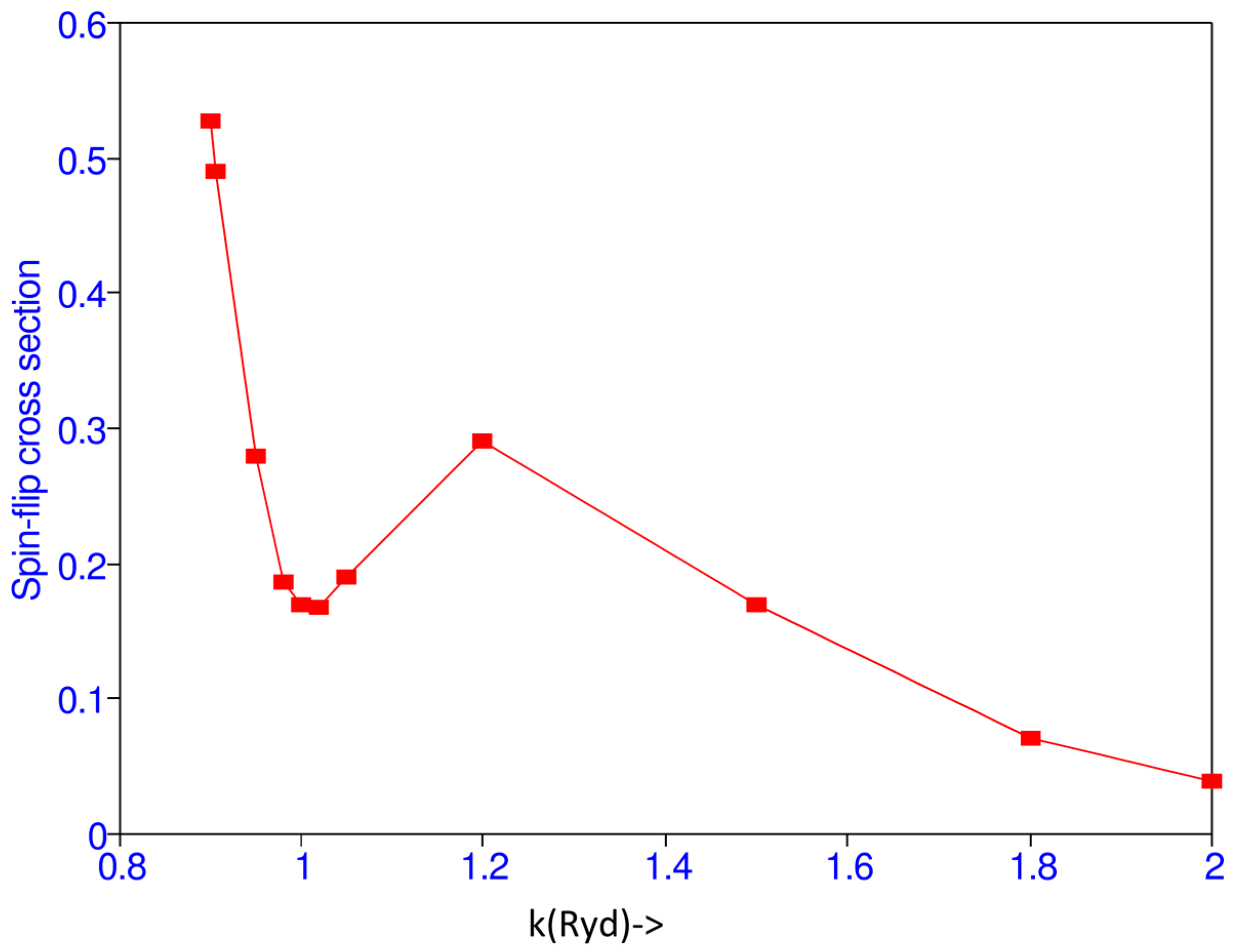
Matrix elements F and G at k = 1.0 are given in Table 3. Cross sections for various values of k are given in Table 4. There is a maximum at the threshold and a minimum at k = 1.02 as shown in Figure 2. The present results have been compared with those obtained by Burke et al. [1] and the present spin-flip cross sections are higher than those obtained in [1].

5. Differential Cross Sections

Differential cross section for excitation is given by:

\frac{d σ}{d Ω} = \frac{k_{f}}{k_{i}} | \sum_{L} (2 L + 1) T_{f i} P_{L} (\cos θ_{f i}) |^{2} .

(17)

Total differential cross section is given by:

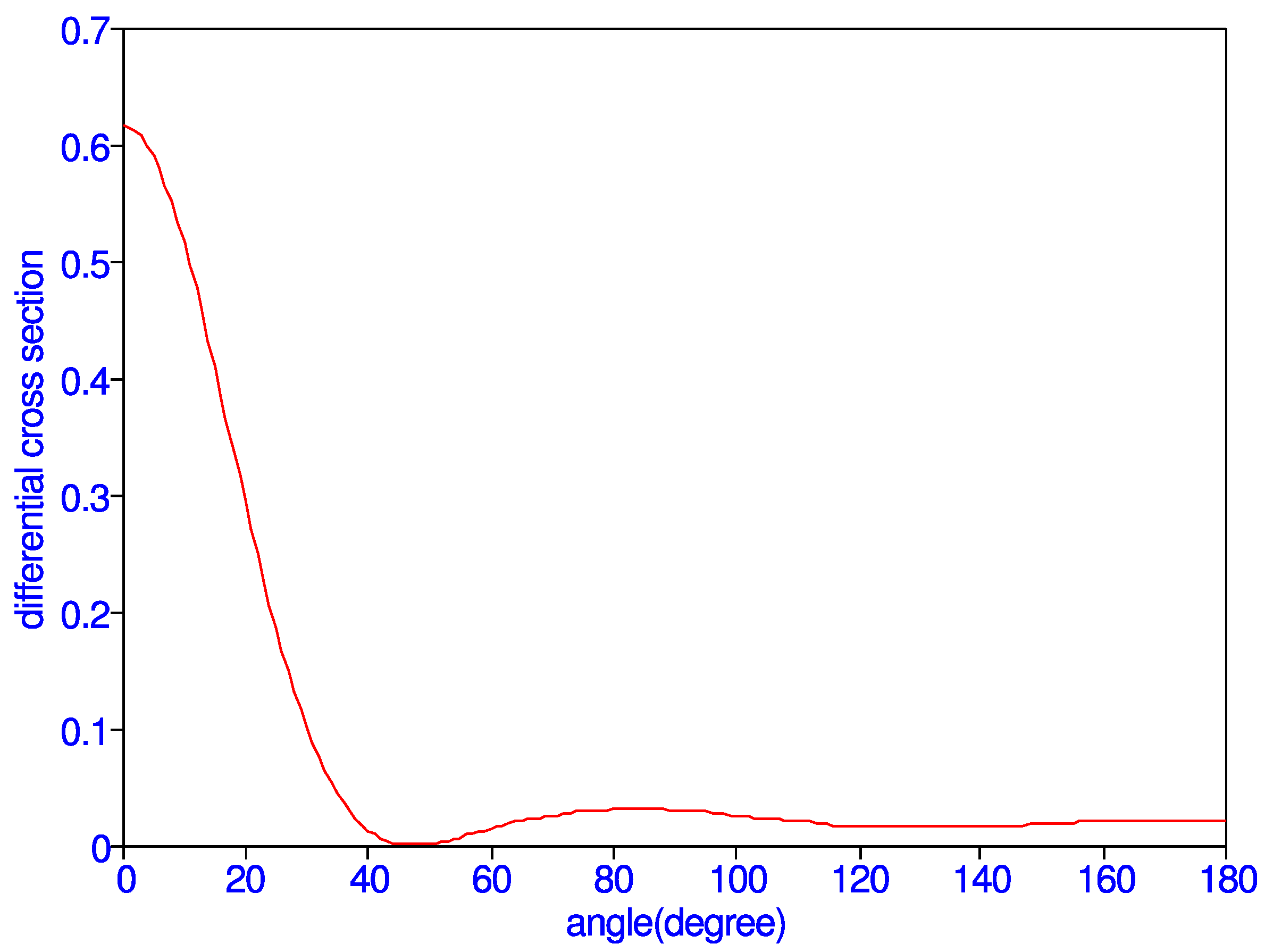
\frac{\partial σ}{\partial Ω} |_{t o t a l} = \frac{\partial σ}{\partial Ω} |_{S i n g l e t} + 3 \frac{\partial σ}{\partial Ω} |_{T r i p l e t} .

(18)

The resulting differential cross section is the sum of the singlet differential cross section and three times the triplet differential cross section. Differential cross sections as a function of scattering angle

θ_{f i}

, in an interval of five degrees, are given in Table 5 for

k_{i}

= 1.0. It is strongly peaked in the forward direction and has a minimum at

θ_{f i}

= 45 degrees, as indicated in Figure 3. The differential cross section rapidly decreases in the beginning as the scattering angle increases. There are no measurements of the differential cross section at this energy to compare with the present results. The total cross section is obtained by multiplying the above equation by

\sin (θ_{f i})

and summing the results for all

θ_{f i}

. Total cross section obtained thus is 0.089648

π a_{0}^{2}

in good agreement with the direct calculation which gives 0.089474

π a_{0}^{2}

.

Differential cross sections over the angular range 20 to 140 degrees have been measured by Williams and Willis [18] for incident energies of 54 to 680 eV. They state that the experimental values do not agree with values predicted by various theories, mentioned in [18]. Differential cross sections at various energies have been calculated using the R-matrix method and Born approximation for higher energies by Scott [19]. However, the results are given in a figure and it is not possible to compare the present results with those given in [19]. Fon et al. [20] have also calculated differential cross sections at k = 1.01, 1.05, and 1.1 using the R-matrix method and their results at 1.01 are lower than the present results at k = 1.0.

6. Conclusions

Calculations for excitation of 2S state of the hydrogen atom from 1S state has been carried out in the distorted-wave approximation using the variational polarized method [9]. At low incident energies, cross sections have been calculated at a fine energy interval. Using the results between k = 0.87 and 2.0, cross sections at other k values can be obtained by interpolation. The present results compare well with those of Burke et al. [1] and agree well with the experimental result of Kauppila et al. [15]. The present results have converged to at least fifth decimal place for most low incident energies.

Acknowledgments

Thanks are extended to R.J. Drachman for helpful discussions and for critical reading of the manuscript. Thanks are also extended to A. Temkin for comments. Calculations were carried out in quadruple precision using the Discover computer at the NASA Center for Computation Science.

Conflicts of Interest

The author declares no conflict of interest.

Appendix A

There are a number of integro-differential equations being solved for scattering functions in this calculation of the excitation of 2S state of atomic hydrogen. They can be solved by an iterative process or by a non-iterative process. A typical integro-differential equation occurring in this calculation can be written in the form:

[\frac{d^{2}}{d r^{2}} + V (r) + k^{2}] u (r) = f (r) \int_{0}^{\infty} g (x) u (x) d x = f (r) C .

(A1)

In the noniterative method of Omidvar [21], we let the function u(r) be of the form:

u (r) = u_{0} (r) + C u_{1} (r) .

(A2)

The constant C represents the definite integral in Equation (A1). Substitution of u(r) in Equation (A1) gives us two equations:

[\frac{d^{2}}{d r^{2}} + V (r) + k^{2}] u_{0} (r) = 0,

(A3)

[\frac{d^{2}}{d r^{2}} + V (r) + k^{2}] u_{1} (r) = f (r) .

(A4)

Now we have two equations which can be solved easily for

u_{0}

and

u_{1}

. Substitution of Equation (A2) in the integral gives

C = \int_{0}^{\infty} g (x) u_{0} (x) d x + C \int_{0}^{\infty} g (x) u_{1} (x) d x = I_{0} + C I_{1}

(A5)

I_{0} = \int_{0}^{\infty} g (x) u_{0} (x) d x,

(A6)

and

I_{1} = \int_{0}^{\infty} g (x) u_{1} (x) d x .

(A7)

Having solved for

u_{0}

and

u_{1}

,

I_{0}

and

I_{1}

can be calculated. From Equation (A5), we can solve for C. We obtain

C = \frac{I_{0}}{(1 - I_{1})} .

(A8)

Putting

u_{0}

,

u_{1}

, and C in Equation (A2), the function u(r) can be calculated. The above procedure can be generalized to any number of integro-differential equations, as has been carried out in [22], where the number of constants were 220, instead of one.

References

Burke, P.G.; Schey, H.M.; Smith, K. Collisions of Slow Electrons and Positrons with Atomic Hydrogen. Phys. Rev. 1963, 129, 1258. [Google Scholar] [CrossRef]
Callaway, J. Scattering of electrons by atomic hydrogen at intermediate energies: Elastic scattering and n = 2 excitation from 12 to 54 eV. Phys. Rev. A 1985, 32, 775–783. [Google Scholar] [CrossRef]
Callaway, J.; Unnikrishnan, K.; Oza, D.H. Optical potential of electron-hydrogen scattering at intermediate energies. Phys. Rev. A 1987, 36, 2576–2584. [Google Scholar] [CrossRef]
Scott, M.P.; Scholz, T.T.; Walters, H.R.; Burke, P.G. Electron scattering by atomic hydrogen at intermediate energies: Integrated elastic, 1s-2s and 1s-2p cross sections. J. Phys. B 1989, 22, 3055–3077. [Google Scholar] [CrossRef]
Bartschat, K.; Hudson, E.T.; Scott, M.P.; Burke, P.G.; Burke, V.M. Electron-atom scattering at low and intermediate energies using a pseudo-state/R-matrix basis. J. Phys. B 1996, 29, 115–123. [Google Scholar] [CrossRef]
Lloyd, M.D.; McDowell, M.R.C. An application of the polarized-orbital approximation to electron impact excitation of atomic hydrogen. J. Phys. B 1969, 2, 1313–1322. [Google Scholar] [CrossRef]
Temkin, A. A Note on the Scattering of Electrons from Atomic Hydrogen. Phys. Rev. 1959, 116, 358. [Google Scholar] [CrossRef]
Poet, R. The exact solution for a simplified model of electrons scattering by hydrogen atoms. J. Phys. B 1978, 11, 3081–3094. [Google Scholar] [CrossRef]
Bhatia, A.K. Hybrid theory of electron-hydrogen elastic scattering. Phys. Rev. A 2007, 75, 032713. [Google Scholar] [CrossRef]
Bhatia, A.K. Application of P-wave hybrid theory to the scattering of electrons from He⁺ and resonances in He and H⁻. Phys. Rev. A 2012, 86, 032709. [Google Scholar] [CrossRef]
Bhatia, A.K. Hybrid theory of P-wave electron-Li⁺ elastic scattering and photoabsorption in two-electron systems. Phys. Rev. A 2013, 87, 042705. [Google Scholar] [CrossRef]
Temkin, A.; Lamkin, J.C. Application of the Method of Polarized Orbitals to the Scattering of Electrons from Hydrogen. Phys. Rev. 1961, 121, 788–794. [Google Scholar] [CrossRef]
Shertzer, J.; Temkin, A. Direct calculation of the scattering amplitude without partial-wave analysis. III. Inclusion of correlation effects. Phys. Rev. A 2006, 74, 052701. [Google Scholar] [CrossRef]
McCarthy, I.E.; Saha, B.C.; Stelbovics, A.T. The polarization potential in electron-atom scattering. J. Phys. B 1981, 14, 2871–2893. [Google Scholar] [CrossRef]
Kauppila, W.E.; Ott, W.R.; Fite, W.L. Excitation of Atomic Hydrogen to the Metastable 2²S_1/2 State by Electron-Impact. Phys. Rev. A 1970, 1, 1099. [Google Scholar] [CrossRef]
Fite, W.L.; Brachman, R.T. Collisions of Electrons with Hydrogen Atoms. II. Excitation of Lyman-Alpha Radiation. Phys. Rev. 1958, 112, 1141–1151. [Google Scholar] [CrossRef]
Fite, W.L.; Stebbings, R.F.; Brachman, R.T. Collisions of Electrons with Hydrogen Atoms. IV. Excitation of Lyman-Alpha Radiation near Threshold. Phys. Rev. 1959, 116, 356–357. [Google Scholar] [CrossRef]
Williams, J.F.; Willis, B.A. Electron scattering from atomic hydrogen I. Differential cross sections for excitation of n = 2 states. J. Phys. B 1975, 8, 1641–1669. [Google Scholar] [CrossRef]
Scott, B.L. Angular Distributions for e⁻ -H Scattering near the First Inelastic Threshold. Phys. Rev. 1965, 140, A699. [Google Scholar] [CrossRef]
Fon, W.C.; Aggarwal, K.M.; Ratnavelu, K. Electron impact excitation of n = 2 states of atomic hydrogen at energies just above the ionization threshold. J. Phys. B 1992, 25, 2625. [Google Scholar] [CrossRef]
Omidvar, K. 2s and 2p Electron-impact Excitation in Atomic Hydrogen. Phys. Rev. 1964, 133, A970. [Google Scholar] [CrossRef]
Bhatia, A.K. Electron-hydrogen P-wave elastic scattering. Phys. Rev. A 2004, 69, 032714. [Google Scholar] [CrossRef]

Figure 1. (Color online) Total 1S–2S excitation cross section (

π a_{0}^{2})

vs. the incident momentum k (Ryd).

Figure 1. (Color online) Total 1S–2S excitation cross section (

π a_{0}^{2})

vs. the incident momentum k (Ryd).

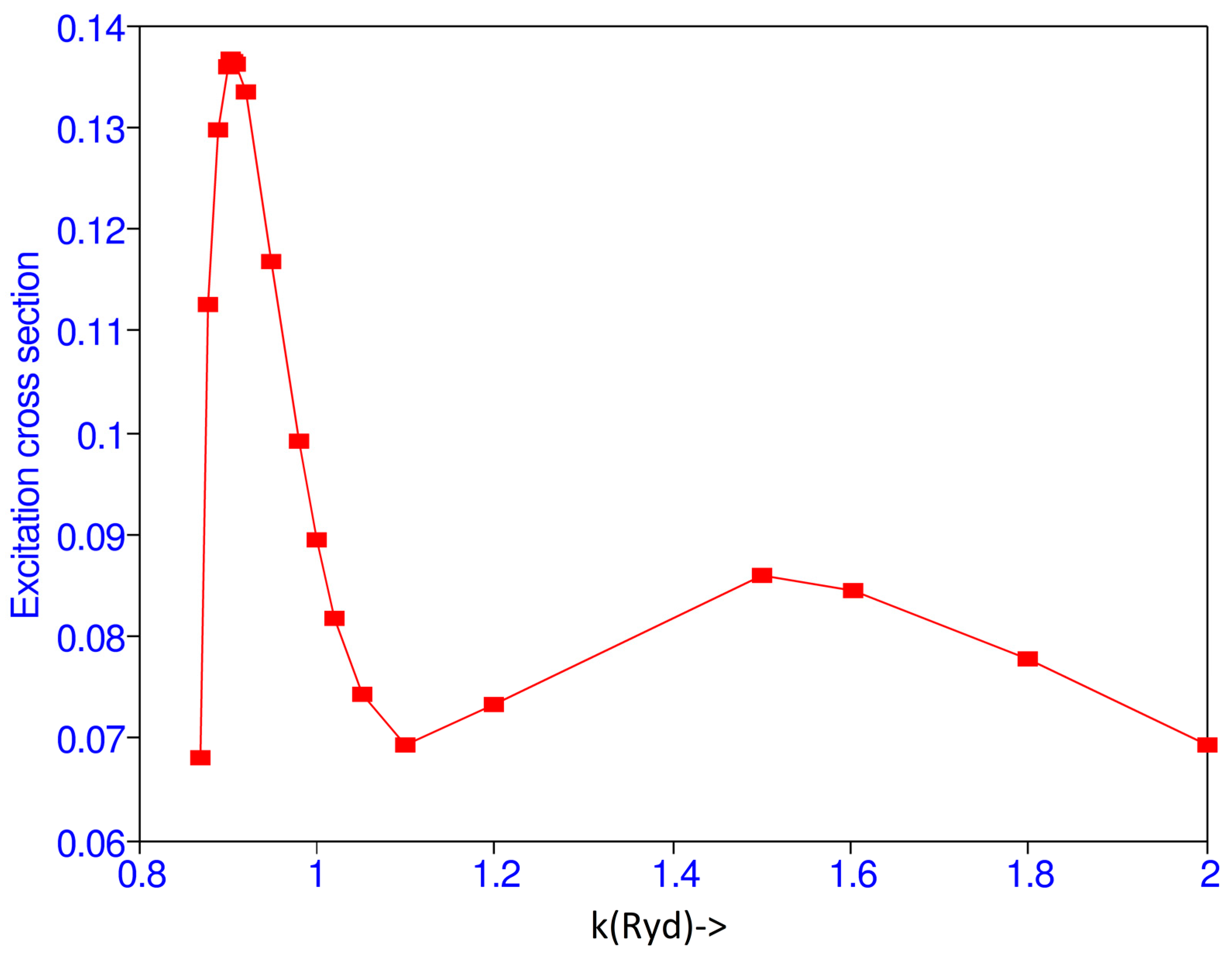
Figure 2. (Color online) Spin-flip cross section

(π a_{0}^{2})

vs. the incident momentum k (Ryd).

Figure 2. (Color online) Spin-flip cross section

(π a_{0}^{2})

vs. the incident momentum k (Ryd).

Figure 3. (Color online) Differential cross section

(π a_{0}^{2} / s r)

vs. angle (degree) at k = 1.0.

Figure 3. (Color online) Differential cross section

(π a_{0}^{2} / s r)

vs. angle (degree) at k = 1.0.

Table 1. Present results (

π a_{0}^{2}

) for excitation of the 2S state of atomic hydrogen using the variational polarized orbital method with Lmax = 8 and comparison with the results obtained in references [1,2,4,6,8]. The superscript indicates interpolated results.

Table 1. Present results (

π a_{0}^{2}

) for excitation of the 2S state of atomic hydrogen using the variational polarized orbital method with Lmax = 8 and comparison with the results obtained in references [1,2,4,6,8]. The superscript indicates interpolated results.

k	Present	Lloyd and McDowell [6]	Poet [8]	Burke et al. [1]	Callaway [2]	Scott et al. [4]
0.87	6.8208(-2)
0.88	1.1267(-1)
0.89	1.2971(-1)
0.90	1.3589(-1)	0.1789		0.09918
0.904	1.3667(-1)
0.905	1.3673(-1)
0.906	1.3662(-1)
0.907	1.3660(-1)
0.91	1.3630(-1)
0.92	1.3345(-1)
0.95	1.1684(-1)
0.98	9.9106(-2)				0.161 ^a
1.00	8.9474(-2)	0.1443	0.0407	0.1783	0.154
1.02	8.1852(-2)				0.150 ^a
1.05	8.4057(-2)				0.142
1.10	6.9444(-2)			0.1654	0.135	0.1087
1.20	7.3317(-2)			0.1349	0.111	0.0986
1.50	8.5797(-2)			0.0891	0.087	0.0867
1.60	8.4611(-2)				0.081 ^a
1.80	7.1804(-2)				0.074 ^a
2.00	6.9460(-2)	0.1198	0.0168	0.06355	0.066	0.0661

Table 2. Cross sections (

π a_{0}^{2}

) for 1 s -> 2 s excitation in the variational P.O. approximation.

Table 2. Cross sections (

π a_{0}^{2}

) for 1 s -> 2 s excitation in the variational P.O. approximation.

k	Present
k	Lmax = 0	Lmax = 1	Lmax = 2	Lmax = 3	Lmax = 4	Lmax = 5	Lmax = 6	Lmax = 7	Lmax = 8
0.87	6.7949(-2)	6.8204(-2)	6.8209(-2)	6.8209(-2)
0.88	1.1107(-1)	1.1246(-1)	1.1255(-1)	1.1267(-1)	1.1267(-1)
0.89	1.2678(-1)	1.2938(-1)	1.2970(-1)	1.2971(-1)	1.2971(-1)
0.90	1.3148(-1)	1.3517(-1)	1.3586(-1)	1.3589(-1)	1.3589(-1)
0.904	1.3166(-1)	1.3574(-1)	1.3663(-1)	1.3667(-1)	1.3667(-1)
0.905	1.3158(-1)	1.3575(-1)	1.3670(-1)	1.3673(-1)	1.3673(-1)
0.906	1.3131(-1)	1.3558(-1)	1.3657(-1)	1.3662(-1)	1.3662(-1)
0.907	1.3115(-1)	1.3550(-1)	1.3655(-1)	1.3660(-1)	1.3660(-1)
0.91	1.3039(-1)	1.3501(-1)	1.3624(-1)	1.3630(-1)	1.3630(-1)
0.92	1.2602(-1)	1.3144(-1)	1.3333(-1)	1.3344(-1)	1.3345(-1)	1.3345(-1)
0.95	1.0447(-1)	1.1187(-1)	1.1638(-1)	1.1681(-1)	1.1684(-1)	1.1684(-1)	1.1684(-1)
0.98	8.0886(-2)	9.0296(-2)	9.8005(-2)	9.898(-2)	9.9093(-2)	9.9105(-2)	9.9105(-2)	9.9105(-2)
1.00	6.6852(-2)	7.7800(-2)	8.7768(-2)	8.9260(-2)	8.9447(-2)	8.9471(-2)	8.9474(-2)	8.9474(-2)
1.02	5.4526(-2)	6.7197(-2)	7.9401(-2)	8.1502(-2)	8.1801(-2)	8.1844(-2)	8.1851(-2)	8.1852(-2)
1.05	3.9620(-2)	5.5101(-2)	7.0508(-2)	7.3670(-2)	7.4202(-2)	7.4290(-2)	7.4305(-2)	7.4308(-2)
1.10	2.2524(-2)	4.2752(-2)	6.2890(-2)	6.8079(-2)	6.9165(-2)	6.9384(-2)	6.3431(-2)	6.9441(-2)	6.9444(-2)
1.20	7.0712(-3)	3.4327(-2)	6.0266(-2)	6.9638(-2)	7.2324-2)	7.3047(-2)	7.3224(-2)	7.3300(-2)	7.3317(-2)
1.50	3.0064(-3)	2.9985(-2)	5.6548(-2)	7.2552(-2)	8.0324(-2)	8.3709(-2)	8.5124(-2)	8.5714(-2)	8.5967(-2)
1.60	3.2974(-3)	2.7537(-2)	5.2116(-2)	6.8368(-2)	7.7147(-2)	8.1383(-2)	8.3328(-2)	8.4208(-2)	8.4612(-2)
1.80	3.2385(-3)	2.2129(-2)	4.2387(-2)	5.7648(-2)	6.7307(-2)	7.2763(-2)	7.5671(-2)	7.7176(-2)	7.7951(-2)
2.00	2.7917(-3)	1.7333(-2)	3.3707(-2)	4.7147(-2)	5.6640(-2)	6.2647(-2)	6.6235(-2)	6.8297(-2)	6.9461(-2)

Table 3. Matrix element for k = 1.0.

L	F	G
0	3.5686(-1)	4.6042(-2)
1	−2.0022(-1)	−9.2426(-2)
2	−9.7205(-2)	−1.7338(-1)
3	−4.6353(-2)	−7.9044(-2)
4	−2.1528(-2)	−3.1113(-2)
5	−9.5763(-3)	−1.1964(-2)
6	−4.1782(-3)	−4.7157(-3)
7	−1.8169(-3)	−1.9301(-3)
8	−7.9477(-4)	−8.1743(-4)

Table 4. Present results for spin-flip cross sections

(π a_{0}^{2})

for various values of k and comparison with the results of [1].

Table 4. Present results for spin-flip cross sections

(π a_{0}^{2})

for various values of k and comparison with the results of [1].

k	Present	Burke et al. [1]
0.90	5.2831(-1)	0.157
0.905	4.9029(-1)
0.95	2.7794(-1)
0.98	1.8597(-1)
1.0	1.6885(-1)	0.2212
1.02	1.6641(-1)
1.05	1.8922(-1)
1.1	2.1959(-1)
1.2	2.8980(-1)	0.1146
1.5	1.6894(-1)	0.0285
1.8	7.0457(-2)
2.0	3.8774(-2)	0.0059

Table 5. Differential cross section (

π a_{0}^{2}

/sr) at k = 1.0 at various scattering angles.

Table 5. Differential cross section (

π a_{0}^{2}

/sr) at k = 1.0 at various scattering angles.

$θ_{f i}$	$\frac{\partial σ}{d Ω}$	$θ_{f i}$	$\frac{\partial σ}{d Ω}$	$θ_{f i}$	$\frac{\partial σ}{d Ω}$
0	6.1752(-1)	65	2.1103(-2)	130	1.6477(-2)
5	5.9068(-1)	70	2.5993(-2)	135	1.6807(-2)
10	5.1623(-1)	75	2.9160-2)	140	1.7405(-2)
15	4.1029(-1)	80	3.0793(-2)	145	1.8120(-2)
20	2.9386(-1)	85	3.1106(-2)	150	1.8854(-2)
25	1.8651(-1)	90	3.0280(-2)	155	1.9557(-2)
30	1.0164(-1)	95	2.8520(-2)	160	2.0211(-2)
35	4.4444(-2)	100	2.6109(-2)	165	2.0804(-2)
40	1.3019(-2)	105	2.3419(-2)	170	2.1298(-2)
45	1.1171(-3)	110	2.0854(-2)	175	2.1634(-2)
50	1.3008(-3)	115	1.8754(-2)	180	2.1754(-2)
55	7.2108(-3)	120	1.7321(-2)
60	1.4565(-2)	125	1.6593(-2)

© 2018 by the author. Licensee MDPI, Basel, Switzerland. This article is an open access article distributed under the terms and conditions of the Creative Commons Attribution (CC BY) license (http://creativecommons.org/licenses/by/4.0/).

Share and Cite

MDPI and ACS Style

Bhatia, A.K. Excitation of the 2S State of Atomic Hydrogen by Electron Impact. Atoms 2018, 6, 7. https://doi.org/10.3390/atoms6010007

AMA Style

Bhatia AK. Excitation of the 2S State of Atomic Hydrogen by Electron Impact. Atoms. 2018; 6(1):7. https://doi.org/10.3390/atoms6010007

Chicago/Turabian Style

Bhatia, Anand K. 2018. "Excitation of the 2S State of Atomic Hydrogen by Electron Impact" Atoms 6, no. 1: 7. https://doi.org/10.3390/atoms6010007

Note that from the first issue of 2016, this journal uses article numbers instead of page numbers. See further details here.

Article Menu

Excitation of the 2S State of Atomic Hydrogen by Electron Impact

Abstract

1. Introduction

2. Calculations

3. Cross Sections

4. Spin-Flip Cross Section

5. Differential Cross Sections

6. Conclusions

Acknowledgments

Conflicts of Interest

Appendix A

References

Share and Cite

Article Metrics

Article Access Statistics

Further Information

Guidelines

MDPI Initiatives

Follow MDPI