Quantum and Semiclassical Stark Widths for Ar VII Spectral Lines


1
Laboratoire Dynamique Moléculaire et Matériaux Photoniques, GRePAA, École Nationale Supérieure d’ingénieurs de Tunis, University of Tunis, Tunis 1008, Tunisia
2
LDMMP, GRePAA, Faculté des Sciences de Bizerte, University of Carthage, Bizerte 7021, Tunisia
3
Sorbonne Université, Observatoire de Paris, Université PSL, CNRS, LERMA, F-92190 Meudon, France
4
Astronomical Observatory, Volgina 7, 11060 Belgrade, Serbia
*
Author to whom correspondence should be addressed.
†
Current address: Astronomical Observatory, Volgina 7, 11060 Belgrade, Serbia.
Atoms 2018, 6(2), 20; https://doi.org/10.3390/atoms6020020
Submission received: 15 March 2018
/
Revised: 6 April 2018
/
Accepted: 10 April 2018
/
Published: 16 April 2018
(This article belongs to the Special Issue Spectral Line Shapes in Astrophysics and Related Topics)
Abstract
:We present in this paper the results of a theoretical study of electron impact broadening for several lines of the Ar VII ion. The results have been obtained using our quantum mechanical method and the semiclassical perturbation one. Results are presented for electron density 1018 cm−3 and for electron temperatures ranging from to K required for plasma modeling. Our results have been compared to other semiclassical ones obtained using different sources of atomic data. A study of the strong collisions contributions to line broadening has been performed. The atomic structure and collision data used for the calculations of line broadening are also calculated by our codes and compared to available theoretical results. The agreement found between the two calculations ensures that our line broadening procedure uses adequate structure and collision data.
1. Introduction
Atomic and line broadening data for many elements and their ions are very useful for solving many astrophysical problems, such as the calculations of opacity and radiative transfer [1]. Especially, accurate Stark broadening parameters are important to obtain a reliable modelization of stellar interiors. The Stark broadening mechanism is also important for the investigation, analysis, and modeling of B-type and particularly A-type stellar atmospheres, as well as white dwarf atmospheres [2,3]. Furthermore, the development of computers and instruments, such as the new X-ray space telescope Chandra, has motivated the calculations of line broadening of trace elements in the X-ray wavelength range. It has been shown that analysis of white dwarf atmospheres, where Stark broadening is dominant compared to the thermal Doppler broadening, needs models taking into account heavy element opacity.
In Rauch et al. [4], the authors reported problems encountered in their determination of element abundances: the line cores of the S VI resonance doublet appear too deep to match the observation and they are not well suited for an abundance determination, and the same problem exists in relation to the N V and O VI. This is due to the lack of line broadening data for these ions. Some other data exist, but the required temperatures and electron densities are lacking, and it is necessary to extrapolate such data to obtain the temperatures and densities at the line-forming regions, especially the line cores. This procedure of extrapolation can provide inaccurate results especially in the case of extrapolating to obtain temperatures, since the temperature dependence of line widths may be very different. This lack of data represents an inconvenience for the development of spectral analysis by means of the NLTE model atmosphere techniques. We quote here the conclusion in Rauch et al. [4]: “spectral analysis by means of NLTE model atmospheres has presently arrived at a high level of sophistication, which is now hampered largely by the lack of reliable atomic data and accurate line-broadening tables.”
Astrophysical interest of Ar VII illustrates for example recent discovery of far UV lines of this ion in the spectra of very hot central stars of planetary nebulae and white dwarfs [5]. In this article, the authors have also shown the importance of the line broadening data for this element in its various ionization stages. Argon also has an important role in plasma technological applications and devices [6]. It produces favorable conditions for very stable discharges and is also very often used as a carrier gas in plasma, which contains a mixture of other gases. Thus, the knowledge of the Stark broadening parameters of neutral and ionized argon lines is an important tool for plasma electron density diagnostic.
The Stark broadening calculations in the present work are based on two approaches: the quantum mechanical approach and the semiclassical perturbation one. The quantum mechanical expression for electron impact broadening calculations for intermediate coupling was obtained in Elabidi et al. [7]. The first applications were performed for the 2s3s−2s3p transitions in Be-like ions from nitrogen to neon [8] and for the 3s−3p transitions in Li-like ions from carbon to phosphor [9]. This approach was also used in Elabidi & Sahal-Bréchot [10] to check the dependence on the upper level ionization potential of electron impact widths and in Elabidi et al. [11] to investigate the influence of strong collisions and quadrupolar potential contributions on line broadening. Our quantum approach is an ab initio method; i.e., all the parameters required for the calculations of the line broadening such as radiative atomic data (energy levels, oscillator strengths ...) or collisional data (collision strengths or cross sections, scattering matrices ...) are evaluated during the calculation and not taken from other data sources. We used the sequence of the University College London (UCL) atomic codes SUPERSTRUCTURE/DW/JAJOM that have been used for many years to provide fine energy levels, wavelengths, radiative probability rates, and electron impact collision strengths. Recently, they have been adapted to line broadening calculations [8].
In the present paper, we continue the effort to provide atomic and line broadening data for argon ions. Quantum Stark broadening of 12 lines of the Ar VII ion have been calculated using 9 configurations (1s22s22p6: 3s2, 3s3p, 3p2, 3s3d, 3p3d, 3s4s, 3s4p, 3s4d, and 3s5s). Our calculations have been made for a set of temperatures ranging from to K. These parameters will be useful for a more accurate determination of photospheric properties. We perform also a semiclassical calculations for these lines using our atomic data from the code SUPERSTRUCTURE. We compare these results to the semiclassical ones [12], for which the atomic structure has been calculated with the Bates and Damgaard approximation [13].
2. Outline of the Theory and Computational Procedure
2.1. Quantum Mechanical Formalism
We present here an outline of our quantum formalism for electron impact broadening. More details can be found elsewhere [7,8]. The calculations are made within the frame of the impact approximation, which means that the time interval between collisions is much longer than the duration of a collision. The expression of the Full Width at Half Maximum (FWHM) W obtained in Elabidi et al. [8] is:
where is the Boltzmann constant, the electron density, T the electron temperature, and
where + = , + l = and + s = . L and S represent the atomic orbital angular momentum and spin of the target, l is the electron orbital momentum, and the superscript T denotes the quantum numbers of the total electron+ion system. () are the scattering matrix elements for the initial (final) levels, expressed in the intermediate coupling approximation, and are respectively the real and the imaginary parts of the S-matrix element, represent 6–j symbols, and we adopt the notation . Both and are calculated for the same incident electron energy . Equation (1) takes into account the fine structure effects and relativistic corrections resulting from the breakdown of the coupling approximation for the target.
The main goal is the evaluation of the real () and the imaginary parts () of the scattering matrix in the initial I and the final F level. The calculation starts with the study of the atomic structure. The structure problem has been treated using the SUPERSTRUCTURE (SST) code described in Eissner et al. [14], taking into account configuration interaction, where each individual configuration is an expansion in terms of Slater states built from orthonormal orbitals. The radial functions were calculated assuming a scaled Thomas–Fermi–Dirac–Amaldi (TFDA) potential. The potential depends upon parameters which are determined variationally by optimizing the weighted sum of the term energies. Relativistic corrections (spin-orbit, mass, Darwin, and one-body) are introduced according to the Breit–Pauli approach [15] as a perturbation to the non-relativistic Hamiltonian. The SST program also produces the term coupling coefficients (TCCs), which are used to transform the scattering or reactance -matrices to intermediate coupling [7].
The second step is the treatment of the scattering problem. The calculation is carried out in the non-relativistic distorted wave approximation using the UCL distorted wave (DW) program [16]. The reactance matrices are calculated in LS coupling. The program JAJOM [17] uses these reactance matrices and the TCC to calculate collision strengths in intermediate coupling. In the present work, we have transformed JAJOM into JAJPOLARI (Elabidi and Dubau, unpublished results) to produce the collision strengths and the reactance matrices in intermediate coupling, which will be used by the program RtoS (Dubau, unpublished results) to evaluate the real and the imaginary parts of the scattering matrix according to
and
The two expressions (3) and (4) have been deduced from the relation , and such expressions guarantee the unitarity of the S-matrix.
Finally, in the code JAJPOLARI, the reactance matrices in intermediate coupling corresponding to the initial I level are evaluated for each channel and at a total energy . The same procedure is done for but at a total energy . () are the energies of the initial (final) atomic levels. The program RtoS receives -matrices and transforms them into real and imaginary parts of -matrices according to Equations (3) and (4) at total energies and , and combines a given matrix element for an initial level I with a number of matrix element for the final level F. The obtained matrix elements and enter into Equation (2).
The integral over the Maxwell distribution (Equation (1)) is evaluated numerically using a trapezoid integration with a variable step to provide the line width W. The energy step is chosen to be as small as possible around the threshold region where the variation of in (1) is fast. For large energies and far from the threshold region, the variation of becomes slow and then the step is gradually increased.
2.2. Semiclassical Perturbation Method
We give here a detailed description of the semiclassical perturbation formalism for line broadening calculations. The profile is Lorentzian for isolated lines:
where
i and f denote the initial and final atomic states and and their corresponding energies.
The total width at half maximum () in angular frequency units of a spectral line can be expressed as
where is the electron density, the Maxwellian velocity distribution function for electrons, (resp. ) denotes the perturbing levels of the initial state i (resp. final state f). The inelastic cross section (resp. ) can be expressed by an integral over the impact parameter of the transition probability (resp. ) as
where denotes the impact parameter of the incoming electron. The elastic cross section is given by
Strong collisions are evaluated for . The phase shifts and due respectively to the polarization potential () and to the quadrupolar potential (), are given in Section 3 of Chapter 2 in Sahal-Bréchot [18], and is the Debye radius. The cut-offs and are described in Section 1 of Chapter 3 in Sahal-Bréchot [19]. Detailed calculations of the interference term can be found in Formulas 18 and 24–30 on pages 109–110 of Sahal-Bréchot [18]. is the contribution of the Feshbach resonances [20], which concerns only ionized radiating atoms colliding with electrons. It is an extrapolation of the excitation collision strengths (and not the cross-sections) under the threshold by means of the semiclassical limit of the Gailitis approximation (see page 601 of [20] for details of the calculations). A review of the theory, all approximations and the details of applications are given in Sahal-Bréchot et al. [21].
3. Results and Discussions
3.1. Atomic Structure and Electron Scattering Data
We have used the following nine configurations in our calculation: 1s22s22p6: 3s2, 3s3p, 3p2, 3s3d, 3p3d, 3s4s, 3s4p, 3s4d, and 3s5s, which give rise to 38 levels, which are listed in Table 1 with their energies in cm−1. These values have been compared with the observed ones taken from the tables of the National Institute of Standards and Technology database: NIST [22] which are originally from Saloman [23]. We compare also with the energies computed using the multiconfiguration Hartree–Fock method (MCHF) [24] and with those obtained using the AUTOSTRUCTURE code [25]. The averaged disagreement between these three results is less than 1%. We detect an inversion between the two levels 10/13 and 25/26 regarding those of NIST and MCHF. This inversion does not affect the calculations since the agreement is still acceptable (about 5%).
We present also in Table 2 radiative decay rates , weighted oscillator strengths , and line strengths S for some Ar VII lines up to the level 14 (3s3d ). Our values have been compared with those obtained from the AUTOSTRUCTURE code [25], and with those from the SUPERSTRUCTURE code [26] using five configurations (1s22s22p6: 3s2, 3s3p, 3p2, 3s3d, and 3s4s). The averaged difference is about 20% with the results of [25] and about 24% with those of Christensen et al. [26]. Some transitions present a high difference, especially those for which are relatively small (about 106 s−1 and below). The values have been compared only with Christensen et al. [26] and the difference is about 24 %. The values are calculated in [26], but we took them from the database CHIANTI version 8.0 [27].
With the code JAJOM, fine structure collision strengths are calculated for low partial waves l of the incoming electron up to 29. For large partial waves l, this method becomes cumbersome and inaccurate, but their contributions to collision strengths cannot be neglected. For , two different procedures have been used: for dipole transitions, the contribution has been calculated using the JAJOM-CBe code (Dubau, unpublished results) based upon the Coulomb–Bethe formulation of Burgess and Sheorey [28] and adapted to JAJOM approximation. For non-dipole transitions, the contribution has been estimated by the SERIE-GEOM code assuming a geometric series behavior for high partial wave collision strengths [29,30].
We present our collision strengths from the lowest five levels to the first 14 levels in Table 3 at electron energy values 7.779, 13.674, and 23.336 Ry. We compared them with the 5-configurations collision strengths of Christensen et al. [26]. Some important discrepancies exist for transitions involving levels arising from the 3p3 configuration (levels 7, 8, and 9). Except for these transitions, the agreement (averaged over the three energies and all the other transitions) is about 20%. The agreement between our results and those of [26] is the worse for the electron energy 7.779 Ry. This energy is close to the excitation energy of the last calculated level (here the energy 6.80 Ry of the level 38). In this situation, the contribution of elastic collisions (which are mostly due to close/strong collisions) is important. We remark also that the agreement is better for transitions from higher levels: for example, is about 39% for transitions from the level 1, and it is about 15% for transitions from the levels . We note that, in [26], calculations have been carried out for partial waves . This may be the origin of the above disagreement for some transitions (we have taken into account partial waves up to 50 in the present work). The difference in the configurations number may also affect the collision strength values.
3.2. Line Broadening Results
Two methods for line broadening calculations have been used in our work. The first is the quantum mechanical approach (Q), and the second is the semiclassical perturbation method . To evaluate the line broadening through the second method, we need atomic parameters such as energy levels and oscillator strengths. In our SCP calculations (), we have taken atomic data of the code SST [14]. We compare our results (Q and ) to the SCP calculations () performed in [12], where atomic data have been taken from the method of Bates and Damgaard [13]. This method has been used many times with different ions, and it has been shown that the corresponding results (using the Bates and Damgaard or the SST data) are in good agreement with experimental and other theoretical results [31,32,33]. Many of these SCP results have been stored in the database STARK-B [34].
We have performed quantum (Q) and semiclassical perturbation () Stark broadening for 12 lines of Ar VII for electron temperature range ( K and at electron density cm−3. We present our results in Table 4 for transitions between singlets, in Table 5 for the resonance line 3s2 −3s3p , and in Table 6 for transitions between triplets. A comparison was made between our quantum and our semiclassical perturbation results in Table 4 and Table 5. We also included the semiclassical results [12] in Table 6 in our comparison. Table 4 and Table 6 show that the quantum line widths are always higher than the two semiclassical ones ( and ). We also found that, except for the resonance line, the ratio increases and decreases with temperature. The decreasing part starts in general at K. For the resonance line 3s2 −3s3p , the ratio increases with T. As per Table 5, this ratio has the same behavior as that of the other lines (increasing and after decreasing) but starts to decrease for higher temperatures ( K). Table 6 shows that, in all studied cases, the widths are closer to the quantum results than the ones. The disagreement between and results is due to the difference in the source of the used atomic data.
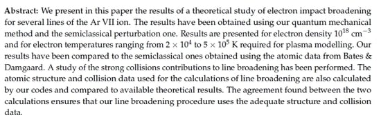
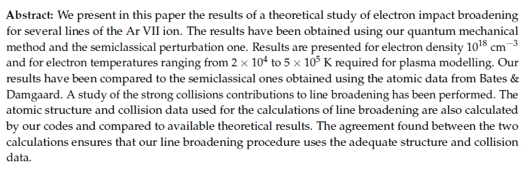
To understand the difference between SCP and quantum calculations, we present also, in Table 4 and Table 6, the contributions of elastic and strong collisions to the line broadening. Firstly, we remark that, for K and except the resonance line, the ratios and decrease with the temperature. Secondly, we see that, for each line, as the elastic and strong collisions contributions decrease, the two results (Q and SCP) become close to each other. For electron temperature K, we can detect in some cases an opposite behavior between and on the one hand and the ratio on the other hand. This may be due to the contributions of resonances that are dominant at low temperatures. These contributions are taken into account differently in the quantum and the semiclassical perturbative methods. Figure 1 shows the behavior of the ratios and with the electron temperature for the 3s3d − 3s4p , 3s3p −3s4d , 3s4p −3s4d , and 3s3p −3s4s transitions. In fact, the Ar VII perturbing levels and are so far from the initial (i) and final (f) levels of the considered transition ( and are high) and, due to this fact, for collisions by electrons, the close collisions are important. Furthermore, with the used temperature values, the ratio is high and consequently, the inelastic cross sections are small compared to the elastic ones that become dominant (mostly due to the close collisions). The perturbative treatment in the semiclassical approach does not correctly estimate this contribution. In that situation, it is necessary to perform more sophisticated calculations such as the quantum ones. We have shown in Elabidi et al. [11], through extensive comparisons between quantum and semiclassical Stark broadening of Ar XV lines, that the disagreement between the two results increases with the increase in strong collision contributions. Figure 2 displays the Stark widths as a function of the electron temperature at a constant electron density for two selected lines between singlets : 3s2 −3s4p and 3s4p −3s5s and two lines between triplets: 3s3p −3s4d , and 3s3d 3s4p .
The obtained Stark broadening parameters will be useful for the investigation and modeling of the plasma of stellar atmospheres. They will be also important for the investigation of laser-produced and inertial fusion plasmas.
4. Conclusions
We have calculated in the present work quantum and semiclassical perturbation Stark broadening parameters for 12 Ar VII lines at electron temperatures from to K and at electron density cm−3. The structure and collision problem has also been treated for this ion. We have used nine configurations (1s22s22p6: 3s2, 3s3p, 3p2, 3s3d, 3p3d, 3s4s, 3s4p, 3s4d, and 3s5s). The structure and collisional parameters have been used in our quantum mechanical line broadening calculations. Since it is important to check their accuracy, we compared our energies to those of [22], to those obtained by the multiconfiguration Hartree-Fock method [24], and to those obtained from the AUTOSTRUCTURE code [25]. An acceptable agreement was found with the NIST results (better than 1%). We also compared our values with those obtained from the AUTOSTRUCTURE code [25] and with those from the SUPERSTRUCTURE code [26] using five configurations (1s22s22p6: 3s2, 3s3p, 3p2, 3s3d, and 3s4s). The averaged difference is about 20% with the results of [25] and about 24% with those of Christensen et al. [26]. The oscillator strengths have been compared only with the results of Christensen et al. [26], and we found an averaged agreement of about 24%. The electron-ion collision process was also studied, and collision strengths from the lowest five levels to the first 14 levels are presented at three electron energies 7.779 Ry, 13.674 Ry, and 23.336 Ry. The comparison with the collision strengths of Christensen et al. [26] indicates an agreement (averaged over the considered transitions and energies) of about 20%. The reason for the disagreement between the two results could be the difference in the number of the configurations and the difference in the partial waves taken into account in the two calculations. Stark line widths for 12 lines have been calculated using our quantum formalism. We perform also a semiclassical perturbation calculations using the structure data of the SST code. We present other semiclassical widths [12] obtained using the atomic data from Bates and Damgaard [13]. Firstly, the disagreement between the two semiclassical calculations is due to the difference in the source of atomic data. Secondly, we have shown that the disagreement between the quantum and the semiclassical widths increases with the increase in the contributions to line broadening of elastic collisions (which are mostly due to strong collisions). This is because the perturbative treatment in the semiclassical approach does not estimate very well the strong collisions. We hope that the present results can fill the lack of line broadening parameters or improve the available results for the Ar VII ion, which are of interest in the investigation and modeling of astrophysical and laboratory plasmas.
Acknowledgments
This work has been supported by the Tunisian Research Unit UR11ES03 and the French one UMR 8112. It has also been supported by the Paris Observatory and the CNRS. We also acknowledge financial support from the “Programme National de Physique Stellaire” (PNPS) of CNRS/INSU, CEA, and CNES, France. This work has also been supported by the Ministry of Education, Science and Technological Development of Serbia (project 176002). Some results have been taken from the database CHIANTI, which is a collaborative project involving George Mason University, the University of Michigan (USA), and the University of Cambridge (UK).
Author Contributions
R.A. and H.E. performed the calculations; H.E., S.S.B., and M.S.D. analyzed the data; H.E. wrote the paper.
Conflicts of Interest
The authors declare no conflict of interest. The founding sponsors had no role in the design of the study; in the collection, analyses, or interpretation of data; in the writing of the manuscript; or in the decision to publish the results.
References
- Dimitrijević, M.S. Stark broadening in astrophysics (applications of Belgrade school results and collaboration with former Soviet republics. Astron. Astrophys. Trans. 2003, 22, 389–412. [Google Scholar] [CrossRef]
- Popović, L.Č.; Simić, S.; Milovanović, N.; Dimitrijević, M.S. Stark Broadening Effect in Stellar Atmospheres: Nd II Lines. Astrophys. J. Suppl. Ser. 2001, 135, 109–114. [Google Scholar] [CrossRef]
- Dimitrijević, M.S.; Ryabchikova, T.; Simić, Z.; Popović, L.Č.; Dačić, M. The influence of Stark broadening on Cr II spectral line shapes in stellar atmospheres. Astron. Astrophys. 2007, 469, 681–686. [Google Scholar] [CrossRef]
- Rauch, T.; Ziegler, M.; Werner, K.; Kruk, J.W.; Oliveira, C.M.; Putte, D.V.; Mignani, R.P.; Kerber, F. High-resolution FUSE and HST ultraviolet spectroscopy of the white dwarf central star of Sh 2-216. Astron. Astrophys. 2007, 470, 317–329. [Google Scholar] [CrossRef]
- Werner, K.; Rauch, T.; Kruk, J.W. Discovery of photospheric argon in very hot central stars of planetary nebulae and white dwarfs. Astron. Astrophys. 2007, 466, 317–322. [Google Scholar] [CrossRef]
- Djurović, S.; Mar, S.; Peláez, R.J.; Aparicio, J.A. Stark broadening of ultraviolet Ar III spectral lines. Mon. Not. R. Astron. Soc. 2011, 414, 1389–1396. [Google Scholar] [CrossRef]
- Elabidi, H.; Ben Nessib, N.; Sahal-Bréchot, S. Quantum mechanical calculations of the electron-impact broadening of spectral lines for intermediate coupling. J. Phys. B 2004, 37, 63–71. [Google Scholar] [CrossRef]
- Elabidi, H.; Ben Nessib, N.; Cornille, M.; Dubau, J.; Sahal-Bréchot, S. Electron impact broadening of spectral lines in Be-like ions: Quantum calculations. J. Phys. B 2008, 41, 025702. [Google Scholar] [CrossRef]
- Elabidi, H.; Sahal-Bréchot, S.; Ben Nessib, N. Quantum Stark broadening of 3s-3p spectral lines in Li-like ions; Z-scaling and comparison with semi-classical perturbation theory. Eur. Phys. J. D 2009, 54, 51–64. [Google Scholar] [CrossRef]
- Elabidi, H.; Sahal-Bréchot, S. Checking the dependence on the upper level ionization potential of electron impact widths using quantum calculations. Eur. Phys. J. D 2011, 61, 285–290. [Google Scholar] [CrossRef]
- Elabidi, H.; Sahal-Bréchot, S.; Dimitrijević, M.S. Quantum Stark broadening of Ar XV lines. Strong collision and quadrupolar potential contributions. Adv. Res. Space 2014, 54, 1184–1189. [Google Scholar] [CrossRef]
- Dimitrijević, M.S.; Valjarević, A.; Sahal-Bréchot, S. Semiclassical Stark broadening parameters of Ar VII spectral lines. Atoms 2017, 5, 27. [Google Scholar] [CrossRef]
- Bates, D.R.; Damgaard, A. The calculation of the absolute strengths of spectral lines. Phil. Trans. R. Soc. Lond. A 1949, 242, 101–122. [Google Scholar] [CrossRef]
- Eissner, W.; Jones, M.; Nussbaumer, H. Techniques for the calculation of atomic structures and radiative data including relativistic corrections. Comput. Phys. Commun. 1974, 8, 270–306. [Google Scholar] [CrossRef]
- Bethe, H.A.; Salpeter, E.E. Quantum Mechanics of One- and Two-Electron Atoms; Springer: Berlin/Göttingen, Germany, 1957. [Google Scholar]
- Eissner, W. The UCL distorted wave code. Comput. Phys. Commun. 1998, 114, 295–341. [Google Scholar] [CrossRef]
- Saraph, H.E. Fine structure cross sections from reactance matrices. Comput. Phys. Commun. 1972, 4, 256–268. [Google Scholar] [CrossRef]
- Sahal-Bréchot, S. Impact Theory of the Broadening and Shift of Spectral Lines due to Electrons and Ions in a Plasma. Astron. Astrophys. 1969, 1, 91–123. [Google Scholar]
- Sahal-Bréchot, S. Impact Theory of the Broadening and Shift of Spectral Lines due to Electrons and Ions in a Plasma (Continued). Astron. Astrophys. 1969, 2, 322–354. [Google Scholar]
- Fleurier, C.; Sahal-Bréchot, S.; Chapelle, J. Stark profiles of some ion lines of alkaline earth elements. J. Quant. Spectrosc. Radiat. Transfer 1977, 17, 595–603. [Google Scholar]
- Sahal-Bréchot, S.; Dimitrijević, M.S.; Ben Nessib, N. Widths and Shifts of Isolated Lines of Neutral and Ionized Atoms Perturbed by Collisions with Electrons and Ions: An Outline of the Semiclassical Perturbation Method and of the Approximations Used for the Calculations. Atoms 2014, 2, 225–252. [Google Scholar] [CrossRef]
- Kramida, A.; Ralchenko, Y.; Reader, J.; NIST ASD Team. NIST Atomic Spectra Database (Version 5.5.1); National Institute of Standards and Technology: Gaithersburg, MD, USA, 2015. Available online: http://physics.nist.gov/asd (accessed on 8 November 2017).
- Saloman, E.B. Energy Levels and Observed Spectral Lines of Ionized Argon, Ar II through Ar XVIII. J. Phys. Chem. Ref. Data 2010, 39, 033101. [Google Scholar] [CrossRef]
- Froese Fischer, C.; Tachiev, G.; Irimia, A. Relativistic energy levels, lifetimes, and transition probabilities for the sodium-like to argon-like sequences. At. Data Nucl. Data Tables 2006, 92, 607–812. [Google Scholar] [CrossRef]
- Fernández-Menchero, L.; Del Zanna, G.; Badnell, N.R. R-matrix electron-impact excitation data for the Mg-like iso-electronic sequence. Astron. Astrophys. 2014, 572, A115. [Google Scholar] [CrossRef]
- Christensen, R.B.; Norcross, D.W.; Pradhan, A.K. Electron-impact excitation of ions in the magnesium sequence. II. SV, ArVII, CaIX, CrXIII, and NiXVII. Phys. Rev. A 1986, 34, 4704–4715. [Google Scholar] [CrossRef]
- Del Zanna, G.; Dere, K.P.; Young, P.R.; Landi, E.; Mason, H.E. CHIANTI—An atomic database for emission lines. Astron. Astrophys. 2015, 582, A56. [Google Scholar] [CrossRef]
- Burgess, A.; Sheorey, V.B. Electron impact excitation of the resonance lines of alkali-like positive ions. J. Phys. B 1974, 7, 2403–2416. [Google Scholar] [CrossRef]
- Chidichimo, M.C.; Haig, S.P. Electron-impact excitation of quadrupole-allowed transitions in positive ions. Phys. Rev. A 1989, 39, 4991–4997. [Google Scholar] [CrossRef]
- Chidichimo, M.C. Electron-impact excitation of electric octupole transitions in positive ions: Asymptotic behavior of the sum over partial-collision strengths. Phys. Rev. A 1992, 45, 1690–1700. [Google Scholar] [CrossRef] [PubMed]
- Hamdi, R.; Ben Nessib, N.; Dimitrijević, M.S.; Sahal-Bréchot, S. Stark broadening of Pb IV lines. Mon. Not. R. Astron. Soc. 2013, 431, 1039–1047. [Google Scholar] [CrossRef]
- Hamdi, R.; Ben Nessib, N.; Sahal-Bréchot, S.; Dimitrijević, M.S. Stark widths of Ar III spectral lines in the atmospeheres of subdwarfs B stars. Adv. Res. Space 2014, 54, 1223–1230. [Google Scholar] [CrossRef]
- Hamdi, R.; Ben Nessib, N.; Sahal-Bréchot, S.; Dimitrijević, M.S. Stark widths of Ar II spectral lines in the atmospeheres of subdwarfs B stars. Atoms 2017, 5, 26. [Google Scholar] [CrossRef]
- Sahal-Bréchot, S.; Dimitrijević, M.S.; Moreau, N. STARK-B Database. Observatory of Paris, LERMA and Astronomical Observatory of Belgrade. 2017. Available online: http://stark-b.obspm.fr (accessed on 8 November 2017).
Figure 1.
Ratios (●) and (○) as a function of the electron temperature for the transitions: 3s3d − 3s4p (left up), 3s3p −3s4d (right up), 3s4p −3s4d (left down), and 3s3p −3s4s (right down).
Figure 1.
Ratios (●) and (○) as a function of the electron temperature for the transitions: 3s3d − 3s4p (left up), 3s3p −3s4d (right up), 3s4p −3s4d (left down), and 3s3p −3s4s (right down).

Figure 2.
Stark width (FWHM) W as a function of the electron temperature for transitions 3s2 −3s4p (left up) and 3s4p −3s5s (right up) at electron density cm−3, and for transitions 3s3p −3s4d (left down) and 3s3d − 3s4p (right down) at electron density cm−3. ○: Present quantum results. ●: Present SCP results. △: SCP results from [12].


Table 1.
Our present fine-structure energy levels E (in cm−1) for Ar VII compared with those of NIST [22], with those obtained from the multiconfiguration Hartree–Fock method (MCHF) [24], and with those from the R-matrix calculation (AS2014) [25]. Levels denoted by asterisks (*) are inverted compared to the NIST values.
| i | Conf. | Level | E | NIST | MCHF | AS2014 | (%) |
|---|---|---|---|---|---|---|---|
| 1 | 0.0 | 0.0 | 0.0 | 0.0 | − | ||
| 2 | 110,717 | 113,101 | 112,817.66 | 112,070 | 2.1 | ||
| 3 | 111,488 | 113,906 | 113,632.14 | 112,889 | 2.1 | ||
| 4 | 113,088 | 115,590 | 115,324.84 | 114,593 | 2.2 | ||
| 5 | 172,878 | 170,722 | 170,598.08 | 173,751 | 1.3 | ||
| 6 | 263,439 | 264,749 | 264,797.88 | 264,530 | 0.5 | ||
| 7 | 271,494 | 269,836 | 269,688.15 | 270,704 | 0.6 | ||
| 8 | 272,341 | 270,777 | 270,667.14 | 271,641 | 0.6 | ||
| 9 | 273,971 | 272,562 | 272,474.76 | 273,432 | 0.5 | ||
| 10 | 325,254 | 324,104 | 324,950.35 | 326,054 | 0.4 | ||
| 11 | 325,335 | 324,141 | 324,966.00 | 326,141 | 0.4 | ||
| 12 | 325,456 | 324,205 | 325,056.68 | 326,273 | 0.4 | ||
| 13 | 333,116 | 316,717 | 317,014.73 | 320,974 * | 5.2 | ||
| 14 | 384,031 | 370,294 | 371,275.29 | 377,167 | 3.7 | ||
| 15 | 443,952 | 443,362 | 444,508.36 | 444,677 | 0.1 | ||
| 16 | 444,892 | 444,780 | 445,556.29 | 445,701 | 0.0 | ||
| 17 | 446,051 | 446,011 | 446,849.87 | 446,969 | 0.0 | ||
| 18 | 450,025 | 450,477 | 450,808.06 | 451352 | 0.1 | ||
| 19 | 474,314 | 472,282 | 473,009.27 | 475,022 | 0.4 | ||
| 20 | 474,956 | 472,875 | 473,782.67 | 475,699 | 0.4 | ||
| 21 | 475,497 | 473,810 | 474,466.36 | 476,301 | 0.4 | ||
| 22 | 477,133 | 475,217 | 475,932.22 | 477,901 | 0.4 | ||
| 23 | 477,515 | 475,585 | 476,306.50 | 478,313 | 0.4 | ||
| 24 | 477,753 | 475,762 | 476,474.91 | 478,560 | 0.4 | ||
| 25 | 513,685 | 514,076 | 508,971.69 | 511,372 | 0.1 | ||
| 26 | 521,897 | 510,268 | 514,890.47 | 515,169 * | 2.3 | ||
| 27 | 527,518 | 517,105 | 517,788.24 | 524,282 | 2.0 | ||
| 28 | 529,866 | 528,910 | 526,205.45 | 523,618 | 0.2 | ||
| 29 | 567,050 | 563,880 | 568,040.66 | 565,087 | 0.6 | ||
| 30 | 567,287 | 564,418 | 568,275.74 | 565,295 | 0.5 | ||
| 31 | 567,811 | 564,728 | 568,944.94 | 565,840 | 0.5 | ||
| 32 | 576,576 | 569,797 | 570,403.78 | 568,205 | 0.2 | ||
| 33 | 635,209 | 634,605 | 635,580.25 | 632,497 | 0.1 | ||
| 34 | 635,241 | 634,639 | 635,659.10 | 632,562 | 0.1 | ||
| 35 | 635,290 | 634,701 | 635,749.02 | 632,659 | 0.1 | ||
| 36 | 639,087 | 635,295 | 636,353.38 | 633,443 | 0.6 | ||
| 37 | 713,912 | 715,747 | − | 717,638 | 0.3 | ||
| 38 | 719,473 | 714,794 | − | 717,997 | 0.7 |
Table 2.
Present radiative decay rates (in s−1) and weighted oscillator strengths compared to those from Christensen et al. [26] (SST86) and to those from [25] (AS2014) for some Ar VII allowed transitions. Line strengths S are also presented. i and j label the levels as in Table 1.
| AS2014) | SST | SST | S | |||
|---|---|---|---|---|---|---|
| 5.968 × | 7.13 × | 1.65 × | 2.160 × | 5.820 × | 0.000638 | |
| 8.114 × | 8.30 × | 8.21 × | 1.221 × | 1.270 × | 2.325423 | |
| 1.854 × | 2.97 × | 2.39 × | 6.018 × | 7.780 × | 0.013038 | |
| 3.748 × | 6.18 × | 6.07 × | 1.243 × | 2.020 × | 0.027216 | |
| 3.719 × | 4.00 × | 3.98 × | 3.400 × | 3.380 × | 1.235825 | |
| 7.249 × | 6.94 × | 6.93 × | 4.245 × | 4.280 × | 0.873472 | |
| 7.818 × | 1.72 × | 1.02 × | 1.205 × | 1.590 × | 0.000402 | |
| 2.492 × | 2.40 × | 2.35 × | 4.291 × | 4.250 × | 0.874104 | |
| 1.842 × | 1.77 × | 1.74 × | 3.202 × | 3.180 × | 0.655396 | |
| 2.976 × | 2.85 × | 2.84 × | 5.278 × | 5.310 × | 1.090986 | |
| 1.274 × | 1.33 × | 3.65 × | 5.793 × | 1.670 × | 0.000192 | |
| 1.877 × | 1.80 × | 1.77 × | 5.329 × | 5.270 × | 1.079810 | |
| 5.481 × | 5.24 × | 5.22 × | 1.587 × | 1.590 × | 3.248175 | |
| 4.965 × | 8.35 × | 7.11 × | 3.642 × | 5.240 × | 0.011859 | |
| 5.993 × | 5.86 × | 5.92 × | 5.857 × | 5.980 × | 0.898754 | |
| 4.449 × | 4.35 × | 4.40 × | 4.379 × | 4.480 × | 0.674448 | |
| 2.906 × | 2.84 × | 2.88 × | 2.904 × | 2.980 × | 0.045058 | |
| 5.117 × | 5.88 × | 1.52 × | 9.913 × | 2.950 × | 0.000214 | |
| 8.015 × | 7.84 × | 7.92 × | 1.314 × | 1.340 × | 2.022700 | |
| 2.618 × | 2.56 × | 2.60 × | 4.356 × | 4.480 × | 0.675718 | |
| 7.418 × | 7.91 × | 1.15 × | 2.392 × | 3.710 × | 0.000517 | |
| 1.048 × | 1.02 × | 1.04 × | 2.439 × | 2.510 × | 3.781547 | |
| 4.347 × | 9.07 × | 5.79 × | 1.327 × | 2.030 × | 0.000197 | |
| 8.643 × | 6.98 × | 6.97 × | 5.047 × | 4.840 × | 1.036879 | |
| 9.459 × | 9.90 × | 1.40 × | 9.546 × | 1.590 × | 0.001153 | |
| 4.427 × | 4.77 × | 4.47 × | 4.521 × | 5.130 × | 0.000055 | |
| 2.085 × | 1.90 × | 1.88 × | 3.506 × | 3.540 × | 5.466647 |
Table 3.
Our collision strengths (Present) and those from [26] (DW86) where and . i and j label the levels as in Table 1.
| Ry | Ry | Ry | ||||
|---|---|---|---|---|---|---|
| Present | DW86 | Present | DW86 | Present | DW86 | |
| 8.901 × | 9.29 × | 4.523 × | 4.54 × | 2.067 × | 2.01 × | |
| 2.936 × | 2.87 × | 1.652 × | 1.46 × | 9.202 × | 7.08 × | |
| 4.430 × | 4.64 × | 2.251 × | 2.26 × | 1.029 × | 1.00 × | |
| 8.841 × | 8.60 × | 9.848 × | 1.03 × | 1.006 × | 1.21 × | |
| 4.208 × | 3.57 × | 4.712 × | 3.48 × | 5.067 × | 3.17 × | |
| 5.400 × | 1.06× | 2.900 × | 5.40 × | 1.200 × | 2.33 × | |
| 1.560× | 2.81× | 8.400 × | 1.30× | 3.300 × | 4.64 × | |
| 4.102 × | 5.74 × | 4.449 × | 5.38 × | 4.785 × | 4.80 × | |
| 2.239 × | 2.39 × | 1.051 × | 1.10 × | 4.603 × | 4.73 × | |
| 3.731 × | 3.99 × | 1.752 × | 1.84 × | 7.671 × | 7.87 × | |
| 5.222 × | 5.58 × | 2.452 × | 2.57 × | 1.074 × | 1.10 × | |
| 3.460× | 1.28 × | 1.030× | 1.10 × | 5.800 × | 8.06 × | |
| 5.431 × | 7.40 × | 6.408 × | 8.03 × | 7.164 × | 8.46 × | |
| 6.257 × | 9.55 × | 3.113 × | 5.28 × | 1.475 × | 3.03 × | |
| 3.621 × | 2.98 × | 3.562 × | 2.79 × | 3.553 × | 2.50 × | |
| 1.103 × | 1.19 × | 5.152 × | 5.09 × | 2.222 × | 2.13 × | |
| 2.860 × | 2.77 × | 1.381 × | 1.40 × | 5.991 × | 6.05 × | |
| 5.657 × | 2.09 × | 2.784 × | 2.95 × | 1.210 × | 1.27 × | |
| 3.379 × | 3.32 × | 3.796 × | 4.05 × | 3.867 × | 4.70 × | |
| 4.773 × | 6.85 × | 2.338 × | 6.45 × | 1.012 × | 3.57 × | |
| 2.744 × | 2.75 × | 3.272 × | 3.43 × | 3.563 × | 4.10 × | |
| 2.286 × | 4.89 × | 1.027 × | 1.23 × | 4.178 × | 5.19 × | |
| 5.517 × | 6.10 × | 5.424 × | 5.58 × | 5.713 × | 5.14 × | |
| 1.746 × | 1.68 × | 8.200 × | 9.19× | 3.490× | 3.75× | |
| 9.861 × | 1.25 × | 4.171 × | 4.77 × | 1.639 × | 1.85 × | |
| 8.916 × | 7.87 × | 8.398 × | 6.89 × | 8.177 × | 5.96 × | |
| 3.383 × | 3.61 × | 1.603 × | 1.55 × | 7.172 × | 6.55 × | |
| 1.349 × | 1.43 × | 9.775 × | 1.19 × | 7.539 × | 1.10 × | |
| 3.379 × | 3.51 × | 3.926 × | 4.27 × | 4.410 × | 4.89 × | |
| 2.556 × | 2.67 × | 2.857 × | 3.12 × | 2.904 × | 3.60 × | |
| 4.186 × | 4.06 × | 4.695 × | 4.81 × | 4.780 × | 5.63 × | |
| 2.088 × | 2.17 × | 2.467 × | 2.66 × | 2.677 × | 3.15 × | |
| 6.232 × | 6.04 × | 7.416 × | 7.47 × | 8.072 × | 9.00 × | |
| 1.428 × | 1.90 × | 1.231 × | 1.28 × | 1.202 × | 1.09 × | |
| 6.369 × | 6.50 × | 3.504 × | 4.24 × | 2.005 × | 2.75 × | |
| 3.305 × | 3.80 × | 1.675 × | 1.49 × | 9.606 × | 6.27 × | |
| 5.693 × | 6.08 × | 2.671 × | 2.61 × | 1.169 × | 1.10 × | |
| 2.318 × | 2.89 × | 1.793 × | 2.75 × | 1.471 × | 2.74 × | |
| 6.345 × | 7.20 × | 3.119 × | 7.70 × | 1.355 × | 4.21 × | |
| 4.238 × | 4.63 × | 4.751 × | 5.46 × | 4.835 × | 6.23 × | |
| 1.261 × | 1.27 × | 1.414 × | 1.52 × | 1.439 × | 1.76 × | |
| 2.468 × | 2.79 × | 2.679 × | 2.93 × | 2.979 × | 3.16 × | |
| 2.208 × | 2.29 × | 2.581 × | 2.75 × | 2.795 × | 3.23 × | |
| 1.165 × | 1.07 × | 1.382 × | 1.32 × | 1.501 × | 1.62 × | |
| 1.042 × | 1.01 × | 4.917 × | 5.27 × | 2.094 × | 2.16 × | |
| 4.929 × | 6.27 × | 2.100 × | 2.39 × | 8.410 × | 9.45 × | |
| 6.396 × | 6.54 × | 6.502 × | 7.69 × | 6.069 × | 8.82 × | |
| 1.214 × | 1.21 × | 6.841 × | 8.61 × | 3.973 × | 5.89 × | |
| 3.337 × | 2.99 × | 1.671 × | 1.68 × | 7.776 × | 7.31 × | |
| 1.169 × | 1.34 × | 8.954 × | 1.27 × | 7.004 × | 1.27 × | |
| 4.295 × | 4.18 × | 1.955 × | 1.84 × | 8.514 × | 7.74 × | |
| 7.151 × | 6.94 × | 3.279 × | 3.04 × | 1.459 × | 1.25 × | |
| 9.742 × | 9.63 × | 4.322 × | 4.18 × | 1.770 × | 1.69 × | |
| 3.939 × | 4.46 × | 4.478 × | 5.32 × | 4.587 × | 6.12 × | |
| 1.653 × | 1.64 × | 1.990 × | 2.06 × | 2.181 × | 2.54 × | |
Table 4.
Our Stark line widths (FWHM) Q for Ar VII at electron density cm−3 compared to the semiclassical results obtained using the atomic data of the code SST. and are respectively the contributions of elastic and strong collisions to line broadening. T is expressed in 104 K.
Table 4.
Our Stark line widths (FWHM) Q for Ar VII at electron density cm−3 compared to the semiclassical results obtained using the atomic data of the code SST. and are respectively the contributions of elastic and strong collisions to line broadening. T is expressed in 104 K.
| Transition | T | Q (Å) | ||||
|---|---|---|---|---|---|---|
| 2 | 2.684 × | 2.380 × | 0.966 | 0.288 | 1.13 | |
| 5 | 1.872 × | 1.500 × | 0.937 | 0.287 | 1.25 | |
| 3s2 −3s3p | 10 | 1.453 × | 1.070 × | 0.891 | 0.286 | 1.36 |
| Å | 20 | 1.135 × | 7.640 × | 0.789 | 0.282 | 1.49 |
| 30 | 9.875 × | 6.360 × | 0.706 | 0.276 | 1.55 | |
| 50 | 8.322 × | 5.160 × | 0.605 | 0.267 | 1.61 | |
| 2 | 9.941 × | 6.070 × | 0.897 | 0.575 | 1.64 | |
| 5 | 6.242 × | 2.930 × | 0.827 | 0.361 | 2.13 | |
| 3s2 −3s4p | 10 | 4.370 × | 2.110 × | 0.766 | 0.357 | 2.07 |
| Å | 20 | 3.038 × | 1.550 × | 0.689 | 0.345 | 1.96 |
| 30 | 2.445 × | 1.320 × | 0.641 | 0.334 | 1.85 | |
| 50 | 1.848 × | 1.090 × | 0.588 | 0.319 | 1.70 | |
| 2 | 6.322 × | 9.750 × | 0.944 | 0.155 | 6.48 | |
| 5 | 3.923 × | 5.400 × | 0.767 | 0.175 | 7.26 | |
| 3s3p −3s4s | 10 | 2.676 × | 3.190 × | 0.616 | 0.172 | 6.84 |
| Å | 20 | 1.759 × | 2.920 × | 0.472 | 0.162 | 6.02 |
| 30 | 1.344 × | 2.500 × | 0.401 | 0.155 | 5.38 | |
| 50 | 9.332 × | 2.080 × | 0.328 | 0.145 | 4.49 | |
| 2 | 4.517 × | 1.360 × | 0.792 | 0.193 | 3.32 | |
| 5 | 2.942 × | 8.840 × | 0.595 | 0.189 | 3.33 | |
| 3s4p −3s5s | 10 | 1.975 × | 6.570 × | 0.458 | 0.179 | 3.01 |
| Å | 20 | 1.266 × | 5.050 × | 0.359 | 0.166 | 2.51 |
| 30 | 9.671 × | 4.400 × | 0.315 | 0.156 | 2.20 | |
| 50 | 6.843 × | 3.740 × | 0.274 | 0.144 | 1.83 | |
| 2 | 1.910 × | 4.150 × | 0.859 | 0.361 | 4.60 | |
| 5 | 1.355 × | 2.650 × | 0.809 | 0.356 | 5.11 | |
| 3s3d −3s4p | 10 | 1.011 × | 1.930 × | 0.737 | 0.346 | 5.24 |
| Å | 20 | 6.854 × | 1.430 × | 0.661 | 0.335 | 4.79 |
| 30 | 5.206 × | 1.210 × | 0.611 | 0.323 | 4.30 | |
| 50 | 3.602 × | 1.010 × | 0.561 | 0.307 | 3.57 | |
| 2 | 1.779 × | 8.070 × | 0.825 | 0.085 | 2.20 | |
| 5 | 1.119 × | 4.750 × | 0.559 | 0.092 | 2.36 | |
| 3s3p −3s5s | 10 | 7.845 × | 3.520 × | 0.400 | 0.087 | 2.23 |
| Å | 20 | 5.460 × | 2.710 × | 0.282 | 0.081 | 2.01 |
| 30 | 4.390 × | 2.360 × | 0.229 | 0.076 | 1.86 | |
| 50 | 3.303 × | 2.000 × | 0.177 | 0.069 | 1.65 |
Table 5.
Our Stark widths (FWHM) Q for the Ar VII 3s2 −3s3p resonance line at electron density cm−3 compared to the semiclassical results obtained using the atomic data of the code SST. and are respectively the contributions of elastic and strong collisions to line broadening. T is expressed in 105 K.
| Transition | T | Q (Å) | ||||
|---|---|---|---|---|---|---|
| 0.2 | 2.684 × | 2.380 × | 0.966 | 0.288 | 1.13 | |
| 0.5 | 1.872 × | 1.500 × | 0.937 | 0.287 | 1.25 | |
| 1 | 1.453 × | 1.070 × | 0.891 | 0.286 | 1.36 | |
| 2 | 1.135 × | 7.640 × | 0.789 | 0.282 | 1.49 | |
| 3s2 −3s3p | 3 | 9.875 × | 6.360 × | 0.706 | 0.276 | 1.55 |
| Å | 5 | 8.322 × | 5.160 × | 0.605 | 0.267 | 1.61 |
| 7.5 | 7.271 × | 4.430 × | 0.537 | 0.255 | 1.64 | |
| 10 | 6.593 × | 4.020 × | 0.494 | 0.245 | 1.64 | |
| 15 | 5.699 × | 3.530 × | 0.444 | 0.232 | 1.61 | |
| 30 | 4.284 × | 2.890 × | 0.389 | 0.211 | 1.48 | |
| 50 | 3.327 × | 2.530 × | 0.366 | 0.199 | 1.32 |
Table 6.
Same as in Table 4 but we add the semiclassical results obtained in Dimitrijević et al. [12] using the atomic data from Bates and Damgaard [13]. Electron density is cm−3 and T is expressed in 104 K.
| Transition | T | Q | ||||||
|---|---|---|---|---|---|---|---|---|
| 2 | 7.510 × | 4.83 × | 4.21 × | 1.55 | 0.889 | 0.444 | 1.77 | |
| 5 | 4.748 × | 2.86 × | 2.49 × | 1.66 | 0.877 | 0.475 | 1.90 | |
| 3s3p −3s4d | 10 | 3.369 × | 2.04 × | 1.81 × | 1.65 | 0.861 | 0.472 | 1.85 |
| Å | 20 | 2.389 × | 1.48 × | 1.35 × | 1.62 | 0.823 | 0.461 | 1.77 |
| 30 | 1.967 × | 1.25 × | 1.15 × | 1.47 | 0.798 | 0.453 | 1.70 | |
| 50 | 1.532 × | 1.02 × | 9.51 × | 1.50 | 0.764 | 0.437 | 1.61 | |
| 2 | 1.613 × | 3.76 × | 3.09 × | 4.29 | 0.901 | 0.457 | 5.22 | |
| 5 | 1.061 × | 2.38 × | 1.99 × | 4.46 | 0.873 | 0.455 | 5.33 | |
| 3s4p −3s4d | 10 | 7.141 × | 1.71 × | 1.45 × | 4.18 | 0.824 | 0.448 | 4.92 |
| Å | 20 | 4.285 × | 1.26 × | 1.08 × | 3.40 | 0.767 | 0.435 | 3.97 |
| 30 | 3.073 × | 1.07 × | 9.27 × | 2.87 | 0.740 | 0.424 | 3.31 | |
| 50 | 2.013 × | 8.87 × | 7.77 × | 2.27 | 0.705 | 0.406 | 2.59 | |
| 2 | 7.585 × | 2.33 × | 1.84 × | 3.26 | 0.928 | 0.406 | 4.12 | |
| 5 | 4.562 × | 1.52 × | 1.16 × | 3.00 | 0.878 | 0.397 | 3.93 | |
| 3s3d −3s4p | 10 | 2.896 × | 1.10 × | 8.35 × | 2.64 | 0.809 | 0.389 | 3.47 |
| Å | 20 | 1.806 × | 8.14 × | 6.12 × | 2.22 | 0.723 | 0.375 | 2.95 |
| 30 | 1.389 × | 6.91 × | 5.18 × | 2.01 | 0.675 | 0.364 | 2.68 | |
| 50 | 1.040 × | 5.73 × | 4.27 × | 1.82 | 0.625 | 0.346 | 2.43 | |
| 2 | 7.605 × | 5.36 × | 5.34 × | 1.42 | 0.942 | 0.337 | 1.42 | |
| 5 | 5.453 × | 3.44 × | 3.33 × | 1.59 | 0.863 | 0.331 | 1.64 | |
| 3s4s −3s4p | 10 | 4.272 × | 2.49 × | 2.40 × | 1.72 | 0.757 | 0.326 | 1.78 |
| Å | 20 | 3.336 × | 1.85 × | 1.79 × | 1.80 | 0.632 | 0.309 | 1.86 |
| 30 | 2.871 × | 1.59 × | 1.53 × | 1.81 | 0.577 | 0.298 | 1.88 | |
| 50 | 2.350 × | 1.33 × | 1.28 × | 1.77 | 0.518 | 0.281 | 1.84 | |
| 2 | 1.396 × | 8.72 × | 5.06 × | 1.56 | 0.996 | 0.358 | 2.75 | |
| 5 | 8.893 × | 5.35 × | 2.68 × | 1.66 | 0.947 | 0.368 | 3.30 | |
| 3s3p −3s4s | 10 | 6.351 × | 3.80 × | 1.91 × | 1.67 | 0.860 | 0.368 | 3.31 |
| Å | 20 | 4.549 × | 2.78 × | 1.41 × | 1.64 | 0.750 | 0.358 | 3.21 |
| 30 | 3.742 × | 2.35 × | 1.21 × | 1.59 | 0.690 | 0.349 | 3.08 | |
| 50 | 2.915 × | 1.94 × | 1.01 × | 1.50 | 0.626 | 0.333 | 2.87 | |
| 2 | 5.727 × | 1.69 × | 9.11 × | 3.39 | 0.986 | 0.334 | 6.24 | |
| 5 | 2.896 × | 9.92 × | 5.85 × | 2.92 | 0.961 | 0.363 | 4.91 | |
| 3s3p −3s3d | 10 | 1.708 × | 7.02 × | 4.17 × | 2.43 | 0.921 | 0.362 | 4.06 |
| Å | 20 | 1.022 × | 5.02 × | 2.96 × | 2.04 | 0.830 | 0.357 | 3.43 |
| 30 | 7.755 × | 4.18 × | 2.45 × | 1.86 | 0.764 | 0.353 | 3.14 | |
| 50 | 5.734 × | 3.37 × | 1.95 × | 1.70 | 0.684 | 0.343 | 2.92 |
© 2018 by the authors. Licensee MDPI, Basel, Switzerland. This article is an open access article distributed under the terms and conditions of the Creative Commons Attribution (CC BY) license (http://creativecommons.org/licenses/by/4.0/).
Share and Cite
MDPI and ACS Style
Aloui, R.; Elabidi, H.; Sahal-Bréchot, S.; Dimitrijević, M.S. Quantum and Semiclassical Stark Widths for Ar VII Spectral Lines. Atoms 2018, 6, 20. https://doi.org/10.3390/atoms6020020
AMA Style
Aloui R, Elabidi H, Sahal-Bréchot S, Dimitrijević MS. Quantum and Semiclassical Stark Widths for Ar VII Spectral Lines. Atoms. 2018; 6(2):20. https://doi.org/10.3390/atoms6020020
Chicago/Turabian StyleAloui, Rihab, Haykel Elabidi, Sylvie Sahal-Bréchot, and Milan S. Dimitrijević. 2018. "Quantum and Semiclassical Stark Widths for Ar VII Spectral Lines" Atoms 6, no. 2: 20. https://doi.org/10.3390/atoms6020020
Note that from the first issue of 2016, this journal uses article numbers instead of page numbers. See further details here.