Matrix Methods for Solving Hartree-Fock Equations in Atomic Structure Calculations and Line Broadening

Abstract

Atomic structure of N-electron atoms is often determined by solving the Hartree-Fock equations, which are a set of integro-differential equations. The integral part of the Hartree-Fock equations treats electron exchange, but the Hartree-Fock equations are not often treated as an integro-differential equation. The exchange term is often approximated as an inhomogeneous or an effective potential so that the Hartree-Fock equations become a set of ordinary differential equations (which can be solved using the usual shooting methods). Because the Hartree-Fock equations are an iterative-refinement method, the inhomogeneous term relies on the previous guess of the wavefunction. In addition, there are numerical complications associated with solving inhomogeneous differential equations. This work uses matrix methods to solve the Hartree-Fock equations as an integro-differential equation. It is well known that a derivative operator can be expressed as a matrix made of finite-difference coefficients; energy eigenvalues and eigenvectors can be obtained by using linear-algebra packages. The integral (exchange) part of the Hartree-Fock equation can be approximated as a sum and written as a matrix. The Hartree-Fock equations can be solved as a matrix that is the sum of the differential and integral matrices. We compare calculations using this method against experiment and standard atomic structure calculations. This matrix method can also be used to solve for free-electron wavefunctions, thus improving how the atoms and free electrons interact. This technique is important for spectral line broadening in two ways: it improves the atomic structure calculations, and it improves the motion of the plasma electrons that collide with the atom.

1. Introduction

Calculations of spectral line broadening are important for a variety of applications, including diagnosing laboratory plasma conditions [1,2], determining temperatures and gravities of white dwarf stars [3], and calculations of stellar opacities [4]. The accuracy of line-broadening calculations is determined by several factors: the accuracy of the atomic structure, the accuracy of the radiator-perturber interaction, and the accuracy of the perturber correlations. If the atomic structure is inaccurate, then the lines will not be in the correct location, and the strengths of the lines may be inaccurate. In addition, the resulting broadening (which depends on both the wavefunctions and the spacing between energy levels) will be affected. If all processes are not considered in the radiator-perturber interaction, then calculations could be missing a broadening mechanism. Lastly, correlations can affect the perturber position thus changing how they interact with the atom.

One particularly important type of interactions that affect all electron-electron interactions is exchange, something that arises due to their indistinguishability. Exchange has been shown to be important for atomic structure [5], atom-electron collisions [6,7,8]), and (most recently) for line-broadening [9]. Line-broadening calculations do not often consider exchange between the radiator and the plasma electrons (though it is included for the calculation of the internal atomic states). There are several reasons for this. First, many use the dipole approximation for the radiator-plasma interaction, which assumes that the radiator and plasma do not occupy the same space, and are therefore distinguishable. Second, many calculations approximate plasma particles as classical, even if they use a more accurate radiator-plasma interaction [10,11,12]. Lastly, many calculations are performed in a high-temperature regime where exchange effects are assumed to be negligible [13,14].

However, some systems, such as lithium-like ions, are known to be dominated by close-range interactions [15]1. From this we can infer that exchange can contribute significantly to the line broadening.

This paper is devoted to exploring wavefunction accuracy, focusing on a technique to improve both atomic structure and free-electron wavefunctions. Most multi-electron wavefunctions are calculated using the Hartree-Fock equations, which are a set of integro-differential equations. However, they are not typically solved as such; they are often solved using techniques of ordinary differential equations (which contain only one variable). We offer a way, using modern computing technology, to solve the integro-differential equations using canned matrix packages, which treats exchange exactly. We begin by looking at changes in the wavefunctions and energy of neutral helium using a matrix method for solving the Hartree-Fock equations with exact exchange. This is a significant improvement since most calculations treat exchange as an inhomogeneous term [21] or treat it using a local-density approximation [22]. We then extend this work to include exchange effects on free-electron wavefunctions. Lastly, we discuss some implications on how collisions of plasma electrons with Li-like ions could change when using our new wavefunctions.

2. The Hartree-Fock Method for Atomic Structure Calculations

Calculation of atomic structure (energy eigenvalues and wavefunctions) of multi-electron atoms or molecules is complicated because no exact analytical solution exists. There are a variety of methods that were introduced to solve multi-electron systems, with the most-studied system being helium-like atoms; see survey in [5]. Probably the most far-reaching method is that of Hartree [23], who used an iterative-refinement method2. The two-electron (non-relativistic) Hamiltonian is

$$\begin{array}{ccc}\hfill H(r_1,r_2)& =& H_0\left(r_1\right)+H_0\left(r_2\right)+V(r_1,r_2)\hfill \\ \hfill H_0\left(r_1\right)& =& -\frac{1}{2}{\nabla }_1^2-\frac{Z}{r_1}\hfill \end{array}$$

(1)

$$\begin{array}{ccc}\hfill V(r_1,r_2)& =& \frac{1}{|{\overrightarrow{r}}_1-{\overrightarrow{r}}_2|},\hfill \end{array}$$

(2)

where Z is the charge of the nucleus, ${\overrightarrow{r}}_1$ and ${\overrightarrow{r}}_2$ are the coordinates of electron 1 and electron 2 respectively. Hartree solved for the motion of one of the electrons by calculating average Coulomb fields due to the second electron. The Hartree method uses an iterative procedure to solve for the atomic structure by solving for the motion of individual electrons with fields due to the other electrons. Each iteration improves the wavefunction; this procedure is repeated until a desired convergence is reached. The steps of the Hartree method can be summarized as

(1)

Assume a wavefunction for the state of interest (hydrogenic is good enough for this step).

(2)

Determine a mean-Coulomb field acting on electron i based on the wavefunctions of the other electron.

(3)

Solve the one-electron Schrödinger equation for electron i in its mean-Coulomb field to generate a new set of wavefunctions.

(4)

Repeat steps (2) and (3) until convergence is achieved.

Hartree’s method, however, neglected the physical indistinguishability of identical particles; this resulted in poor results in matching the helium spectrum. The two-electron Hamiltonian (Equation (1)) is unchanged upon exchange of the positions of electron 1 and electron 2. The wavefunction eigensolution, therefore, must also have this property, such that

$$\begin{array}{ccc}\hfill \Psi ({\overrightarrow{r}}_1,{\overrightarrow{r}}_2)& =& \pm \Psi ({\overrightarrow{r}}_2,{\overrightarrow{r}}_1),\hfill \end{array}$$

(3)

$$\begin{array}{cc}=& \frac{1}{\sqrt{2}}\left[{\psi }_1\left({\overrightarrow{r}}_1\right){\psi }_2\left({\overrightarrow{r}}_2\right)\pm {\psi }_2\left({\overrightarrow{r}}_1\right){\psi }_1\left({\overrightarrow{r}}_2\right)\right],\hfill \end{array}$$

(4)

where ${\psi }_1$ and ${\psi }_2$ are the one-electron wavefunctions for electrons 1 and 2, respectively. The positive symmetry sign is interpreted as the spin-anti-aligned case, while the anti-symmetry choice is the spin-aligned case.

The Hartree-Fock equations [5,21,24] are based on a variational method to minimize the energy of the system using the fully symmetrized wavefunctions in Equation (4), resulting in the following set of differential equations for ${\psi }_1$ and ${\psi }_2$,

$$\begin{array}{ccc}\hfill \left[-\frac{1}{2}{\nabla }_1^2-\frac{Z}{r_1}+V_C\left(r_1\right)-E\right]{\psi }_1\left({\overrightarrow{r}}_1\right)& \approx & \mp \left\{\int d^3{\overrightarrow{r}}_2{\psi }_1\left({\overrightarrow{r}}_2\right)\frac{1}{r_{12}}{\psi }_2\left({\overrightarrow{r}}_2\right)\right\}{\psi }_2\left({\overrightarrow{r}}_1\right)\hfill \end{array}$$

(5)

$$\begin{array}{ccc}\hfill \left[-\frac{1}{2}{\nabla }_2^2-\frac{Z}{r_2}+V_C\left(r_2\right)-E\right]{\psi }_2\left({\overrightarrow{r}}_2\right)& \approx & \mp \left\{\int d^3{\overrightarrow{r}}_1{\psi }_1\left({\overrightarrow{r}}_1\right)\frac{1}{r_{12}}{\psi }_2\left({\overrightarrow{r}}_1\right)\right\}{\psi }_1\left({\overrightarrow{r}}_2\right)\hfill \end{array}$$

(6)

for a two electron system; $V_C$ is the average direct Coulomb potential from the other electron,

$$V_c\left(r_1\right)={\int }_0^{\infty }{d}^3{\overrightarrow{r}}_2{\psi }_2\left({\overrightarrow{r}}_2\right)\frac{1}{r_{12}}{\psi }_2\left({\overrightarrow{r}}_2\right),$$

and the terms in curly brackets on the right-hand side are the exchange terms. Here we have omitted some of the overlap integrals, which are often approximated with Lagrangian multipliers [21]3. The Hartree-Fock equations are some of the most widely-used equations in atomic structure [5,21,25], providing an accurate set of starting wavefunctions and energies.

One source of uncertainty with solving the Hartree-Fock equations is the treatment of the exchange term on the right-hand sides of Equations (5) and (6). Current calculations which treat exchange explicitly approximate these terms as if they are an inhomogeneous term of a differential equation [21,26,27,28], where the differential equation for electron 1 is approximated as

$$\left[-\frac{1}{2}{\nabla }_1^2-\frac{Z}{r_1}+V_C\left(r_1\right)-E\right]{\psi }_1\left({\overrightarrow{r}}_1\right)\approx \mp s\left(r_1\right),$$

(7)

where $s\left(r_1\right)$ is the inhomogeneous term of the differential equation, which contains the exchange term, and its evaluation relies on the previous guess of the new wavefunction for which we are trying to solve. In addition, one must be careful when evaluating an inhomogeneous term numerically [21]. Equation (7) is often solved using the shooting method, which involves matching boundary conditions and searching for eigenvalues.

Contrast Equation (7) with Equation (5), where the function that is being solved is inside the integral on the right-hand side; therefore the Hartree-Fock equations are integro-differential equations. Computing power has now reached a point where integro-differential equations can be solved using finite-difference matrices similar to the one used by Beck [28].

3. Finite Difference Matrix to Solve the Schrödinger Equation for One-Electron Atom

Before we begin discussing solutions to the Hartree-Fock equations, we would like to introduce the idea of using matrices to solve the one-electron Schrödinger equation for a problem where an analytic solution is known. We therefore choose to use finite-difference matrix methods to solve for the hydrogen atom. The non-relativistic hydrogen wavefunction can be separated into radial and spherical coordinates,

$$\psi (r,\theta ,\varphi )=\frac{1}{r}{R}_{nl}\left(r\right)Y_{lm}(\theta ,\varphi ),$$

where the behavior of the angular part is known and well-characterized by the spherical harmonics, and the radial wavefunction, $R_{nl}\left(r\right)$, is the part that needs to be solved. The radial wavefunction is the solution to the Schrödinger equation (atomic units used throughout; $\hslash =1$, $m_e=1$, and $e=1$),

$$\left[-\frac{d^2}{d{r}^2}+\frac{l(l+1)}{r^2}-\frac{2Z}{r}\right]R_{nl}\left(r\right)=2E_n{R}_{nl}$$

(8)

As is shown in Beck [28], the second-order derivative can be represented with finite-difference coefficients,

$$\begin{array}{c}\begin{array}{ccc}\left[\frac{d^2}{d{r}^2}{R}_{nl}\left(r_i\right)\right]\hfill & \approx \hfill & \frac{1}{{(\Delta r)}^2}\left[R_{nl}\left(r_{i+1}\right)+R_{nl}\left(r_{i-1}\right)-2R_{nl}\left(r_i\right)\right]\hfill \\ & \approx \hfill & \frac{1}{{(\Delta r)}^2}\left(\begin{array}{ccc}1& -2& 1\end{array}\right)\left(\begin{array}{c}{R}_{nl}\left(r_{i-1}\right)\\ R_{nl}\left(r_i\right)\\ R_{nl}\left(r_{i+1}\right)\end{array}\right)\hfill \end{array}\hfill \end{array}$$

(9)

which can be written more generally as a matrix (with $r_i$ = $i\Delta r$)

$$\begin{array}{ccc}\hfill \left[\frac{d^2}{d{r}^2}{R}_{nl}\left(r\right)\right]& \approx & \frac{1}{{(\Delta r)}^2}\left(\begin{array}{ccccc}-2& 1& 0& 0& \cdots \\ 1& -2& 1& 0& \cdots \\ 0& 1& -2& 1& \cdots \\ 0& 0& 1& -2& \cdots \\ ⋮& ⋮& ⋮& ⋮& \ddots \end{array}\right)\left(\begin{array}{c}{R}_{nl}(\Delta r)\\ R_{nl}(2\Delta r)\\ R_{nl}(3\Delta r)\\ R_{nl}(4\Delta r)\\ ⋮\end{array}\right).\hfill \end{array}$$

(10)

The potential in which the electron is moving is a diagonal matrix,

$$V\left(r\right)R_{nl}\left(r\right)=\left(\begin{array}{ccccc}V\left(r_1\right)& 0& 0& 0& \cdots \\ 0& V\left(r_2\right)& 0& 0& \cdots \\ 0& 0& V\left(r_3\right)& 0& \cdots \\ 0& 0& 0& V\left(r_4\right)& \cdots \\ ⋮& ⋮& ⋮& ⋮& \ddots \end{array}\right)\left(\begin{array}{c}{R}_{nl}(\Delta r)\\ R_{nl}(2\Delta r)\\ R_{nl}(3\Delta r)\\ R_{nl}(4\Delta r)\\ ⋮\end{array}\right),$$

(11)

where $V\left(r\right)$ is

$$V\left(r\right)=\frac{l(l+1)}{r^2}-2\frac{Z}{r}.$$

The total Hamiltonian will simply be the sum of the differential matrix and the potential matrix. These techniques are well established e.g., [29,30] and could be improved upon by using higher-order finite-difference elements, or using the Numerov method in matrix form.

The advantage of this technique is that any linear-algebra package, such as LAPACK [31], can be used to diagonalize this Hamiltonian to get energies and wavefunctions. As a result, complications with shooting methods, such as trying to match the inner and outer solutions (or having to search for an eigenvalue), are avoided—though at a cost: numerically solving for the eigenvalues and eigenvectors of a large Hamiltonian can become time-consuming (taking anywhere from a few times to hundreds of times longer than a Numerov shooting method, depending on the size of the box and the solver). As with any finite-difference method, smaller $\Delta r$ results in more accurate wavefunctions, but requires a larger matrix to solve, which means the calculation will converge more slowly.

To illustrate the accuracy of the calculations using this method,

Table 1. Numerical Eigenvalue Solutions.

n	$\mathbf{\Delta }\mathit{r}=0.5$	$\mathbf{\Delta }\mathit{r}=0.2$	$\mathbf{\Delta }\mathit{r}=0.1$	$\mathbf{\Delta }\mathit{r}=0.05$	Exact
1	−0.94427	−0.99019	−0.99751	−0.99937	−1.00000
2	−0.24621	−0.24938	−0.24984	−0.24996	−0.25000
3	−0.11035	−0.11098	−0.11108	−0.11110	−0.11111
4	−0.06218	−0.06237	−0.06240	−0.06241	−0.06250

shows the energy eigenvalues of hydrogen assuming a maximum r of 50 Bohr, and compares the accuracy of different $\Delta r$; the Hamiltonians are $N\times N$ matrices where $N=100$, $N=250$, $N=500$, $N=1000$ for $\Delta r=0.5$, $\Delta r=0.2$, $\Delta r=0.1$, $\Delta r=0.05$, respectively (all in units of Bohr distance; 1 Bohr = 5.29$\times {10}^{-9}$ cm).

We see that the errors in the energy eigenvalue for $\Delta r=0.1$ Bohr is roughly 0.2% for the ground state, and less than 0.1% for the excited states, while the $\Delta r=0.05$ Bohr calculation has 0.06% errors in the ground-state energies, and ≤0.02% errors for the excited states.

4. Matrix Form of the Hartree-Fock Equation

To solve for multi-electron systems, we can extend Equation (10) to solve for more than one radial function simultaneously. For example, one can construct a differential matrix for a wavefunction that has two coordinate positions,

$$R(r_1,r_2)=\left(\begin{array}{c}R(\Delta r,\Delta r)\\ R(2\Delta r,\Delta r)\\ R(3\Delta r,\Delta r)\\ ⋮\\ R(\Delta r,2\Delta r)\\ R(2\Delta r,2\Delta r)\\ R(3\Delta r,2\Delta r)\\ ⋮\end{array}\right)$$

If there are N spatial coordinates ($N=r_{max}/\Delta r$), then this means that for two-electron systems, the vector size will be $N^2$ instead of N. Therefore, the most practical method for solving for multi-electron systems is the Hartree-Fock equations—though it is not impossible to solve such a large system on a laptop computer4.

The Hartree-Fock equations (Equations (5) and (6)) contain two additional terms not present in the one-electron Schrödinger equation: the direct and exchange interactions with the other electrons in the system. For the rest of the section, we use the multipole expansion of the Coulomb interaction,

$$\frac{1}{|{\overrightarrow{r}}_1-{\overrightarrow{r}}_2|}=\sum _{k=0}^{\infty }\frac{r_{<}^k}{r_{>}^{k+1}}{P}_k(cos{\gamma }_{12})$$

(12)

where $r_{<}$ and $r_{>}$ are the lesser/greater of $r_1$ and $r_2$, and $P_k$ is a Legendre polynomial, and ${\gamma }_{12}$ is the angle between ${\overrightarrow{r}}_1$ and ${\overrightarrow{r}}_2$.

The direct term is defined as the spherically-averaged potential, which is just the monopole term. The $i^{th}$ electron feels the average monopole interaction from the other electrons

$$V_{dir}\left(r\right)R_i\left(r\right)=R_i\left(r\right)\sum _{j\ne i}{\int }_0^{\infty }d{r}_1{R}_j^{*}\left(r_1\right)R_j\left(r_1\right)\frac{1}{r_{>}},$$

(13)

where $r_{>}$ is the greater of $r_1$ and r. This poses no complications from the treatment in Section 3 due to the fact that the resulting potential is diagonal like Equation (11), and can just be added to the centrifugal and nuclear potentials.

The exchange term is a bit more complicated [5,21],

$$V_{exch}\left(r\right){\psi }_i\left(\overrightarrow{r}\right)=\mp \sum _{j\ne i}\sum _k{\psi }_j\left(\overrightarrow{r}\right){\int }_0^{\infty }{d}^3{\overrightarrow{r}}_1{\psi }_j^{*}\left({\overrightarrow{r}}_1\right)\frac{r_{<}^k}{r_{>}^{k+1}}{P}_k(cos\gamma ){\psi }_i\left({\overrightarrow{r}}_1\right),$$

Using the spherical harmonics, their relationship with the Wigner 3j-symbols, and averaging over all m quantum numbers, the exchange contribution can be reduced to [21],

$$V_{exch}\left(r\right)R_i\left(\overrightarrow{r}\right)=\sum _{j\ne i}\sum _k-\frac{1}{2}{\left(\begin{array}{ccc}{l}_j& k& l_i\\ 0& 0& 0\end{array}\right)}^2{R}_j\left(r\right){\int }_0^{\infty }d{r}_1{R}_j^{*}\left(r_1\right)\frac{r_{<}^k}{r_{>}^{k+1}}{R}_i\left(r_1\right).$$

(14)

We can define the integral with finite difference matrix coefficients in a similar way to the derivative, as discussed in the previous section. The integral in Equation (14) can be discretized as follows (where $r_1$ have been replaced with a spatial index, $x\Delta r$),

$$V\left(r\right)=\sum _{j\ne i}\sum _k{R}_j\left(r\right)\sum _x{R}_j^{*}(x\Delta r){\widehat{V}}^k(r,x\Delta r)R_i(x\Delta r)\Delta r,$$

where

$$\widehat{V}(r_1,r_2)=-\frac{1}{2}{\left(\begin{array}{ccc}{l}_j& k& l_i\\ 0& 0& 0\end{array}\right)}^2\frac{r_{<}^k}{r_{>}^{k+1}}.$$

This can be written as a matrix (omitting the sums over j and k),

$$\begin{array}{c}\hfill \Delta r\left(\begin{array}{cccc}{R}_j(\Delta r)R_j^{*}(\Delta r){\widehat{V}}^k(\Delta r,\Delta r)& R_j(\Delta r)R_j^{*}(2\Delta r){\widehat{V}}^k(\Delta r,2\Delta r)& R_j(\Delta r)R_j^{*}(3\Delta r){\widehat{V}}^k(\Delta r,3\Delta r)& \cdots \\ R_j(2\Delta r)R_j^{*}(\Delta r){\widehat{V}}^k(2\Delta r,\Delta r)& R_j(2\Delta r)R_j^{*}(2\Delta r){\widehat{V}}^k(2\Delta r,2\Delta r)& R_j(2\Delta r)R_j^{*}(3\Delta r){\widehat{V}}^k(2\Delta r,3\Delta r)& \cdots \\ R_j(3\Delta r)R_j^{*}(\Delta r){\widehat{V}}^k(3\Delta r,\Delta r)& R_j(3\Delta r)R_j^{*}(2\Delta r){\widehat{V}}^k(3\Delta r,2\Delta r)& R_j(3\Delta r)R_j^{*}(3\Delta r){\widehat{V}}^k(3\Delta r,3\Delta r)& \cdots \\ R_j(4\Delta r)R_j^{*}(\Delta r){\widehat{V}}^k(4\Delta r,\Delta r)& R_j(4\Delta r)R_j^{*}(2\Delta r){\widehat{V}}^k(4\Delta r,2\Delta r)& R_j(4\Delta r)R_j^{*}(3\Delta r){\widehat{V}}^k(4\Delta r,3\Delta r)& \cdots \\ ⋮& ⋮& ⋮& \ddots \end{array}\right)\left(\begin{array}{c}{R}_i(\Delta r)\\ R_i(2\Delta r)\\ R_i(3\Delta r)\\ R_i(4\Delta r)\\ ⋮\end{array}\right).\end{array}$$

(15)

This method still requires knowledge of the other electrons, but now this equation solves for $R_i\left(r\right)$ once per iteration. It should be stated that the shooting method, which requires multiple integrations on its inhomogeneous term, is still faster than the matrix method. However, as we stated above, the matrix method finds the eigenvalues automatically, does not require any delicate handling of the numerics surrounding an inhomogeneous term, and it is self consistent, needing no information about $R_i$ from a previous guess that the shooting method requires.

The numerical results of using this Hartree-Fock matrix method are plotted in Figure 1 for the spin-aligned (ortho-helium) and spin-anti-aligned (para-helium) cases. These results differ from the wavefunctions calculated from Cowan [21], even for the average (of para- and ortho-helium). The biggest difference is in the size of the part that overlaps with the 1s electron, as evident in Figure 2. This means that Cowan’s code predicts a wavefunction that is more likely to occupy the same space as the 1s electron. Orthogonality, defined as

$${\int }_0^{\infty }dr{R}_i\left(r\right)R_j\left(r\right)={\delta }_{ij},$$

(16)

between the 1s and 2s electrons of the 1s2s configuration offers a useful metric for comparison. Cowan’s code uses Lagrangian multipliers to force orthogonality. Our calculation of LS-averaged wavefunctions produce overlap integrals (Equation (16) for the 2s and 1s states that are 0.02. However, if we calculate each LS term (ortho- and para-helium), the 1s and 2s ortho-helium (spin-aligned) triplet states have overlap integrals that are less than 0.001 (comparable to Cowan [21]), but the 1s and 2s states of the para-helium singlet state are not orthogonal (overlap integral is 0.08); this have been observed before in Hartree-Fock calculations [24,32].

The energies are also different—and this may be where these details matter most. In

Table 2. Energy difference between $2s^{3}S$ and $2s^{1}S$ in Ry.

Cowan	Hartree-Fock with Exact Exchange	Direct Two-Electron Solution	Measured [33,34]
0.06749	0.06158	0.0602	0.05857

, we compare the different calculations for the energy separation of the two different LS terms (para- and ortho-helium) of the 2s state of helium to the reference value from NIST [33,34]. Our matrix Hartree-Fock method reduces the discrepancy with experiment to 5% from the 15% discrepancy from Cowan [21]; see Table 2. A direct numerical two-electron solution (where we expand Equation (10) to two dimensions and include a monopolar repulsion term; this is not the Hartree-Fock equations) agrees well with the reference value.

5. Extension to Free-Electron Wavefunctions

This same technique can also be used to calculate free-electron wavefunctions. However, the problem is slightly different than the bound-electron problem. First, the eigenvalue is known, and second, the outer boundary condition is not zero. To accommodate this, we move the energy ($E=\frac{1}{2}{k}^2$) to the other side of Equation (8), so that the system for which we are solving is

$$(H-E)\psi \left(r\right)=0$$

We then use a matrix solver ($Ax=b$), rather than an eigenvalue solver, and set the b vector equal to zero except for the final value, which is set to 1,

$$b=\left(\begin{array}{c}0\\ 0\\ 0\\ ⋮\\ 0\\ 1\end{array}\right).$$

This choice will ensure that the wavefunction does not decay to zero at the outer-most boundary.

The changes in the free-electron wavefunction are shown in Figure 3 and Figure 4 for a distorted-wave treatment, where we assume that the atom is not perturbed by the presence of the free-electron. Figure 3 shows the free electron reacting to a hydrogen atom in the $2s$ state, while Figure 4 shows the free electron reacting to a lithium atom in the $1s^{2}2s$ configuration. In these figures, we also plot the plane-wave solution for the same k state, and a local-density-approximation (LDA) for the exchange contribution [21,35,36]. The changes in the wavefunction in Figure 3 are fairly minor, and the LDA gives fairly reasonable amplitudes for the inner 5 Bohr of the wavefunction. The lithium wavefunctions calculated with an LDA, on the other hand, are not nearly as good; the amplitudes of the exact exchange are lower by 30–50%. This means that if one were trying to accurately calculate the effects of penetrating collisions for multi-electron—meaning more than one electron—systems, the LDA wavefunction may not be accurate enough depending on the application.

The differences between the three treatments (Coulomb/Plane wave, LDA, and exact exchange) become less important as the charge of the atom increases. For example, in Li-like boron, the differences are much less pronounced because the nuclear charge becomes the dominant contribution to the potential.

6. Application to Spectral Line Broadening

The line broadening of spectral lines is due to the radiator interacting with its environment. Therefore, the accuracy of spectral line broadening depends on three primary details: the atomic structure, the description of the plasma ensemble properties, and the way the plasma and atoms interact. The work here has an impact on spectral line broadening in two ways: the atomic structure and the behavior of plasma electrons when they impact the radiator.

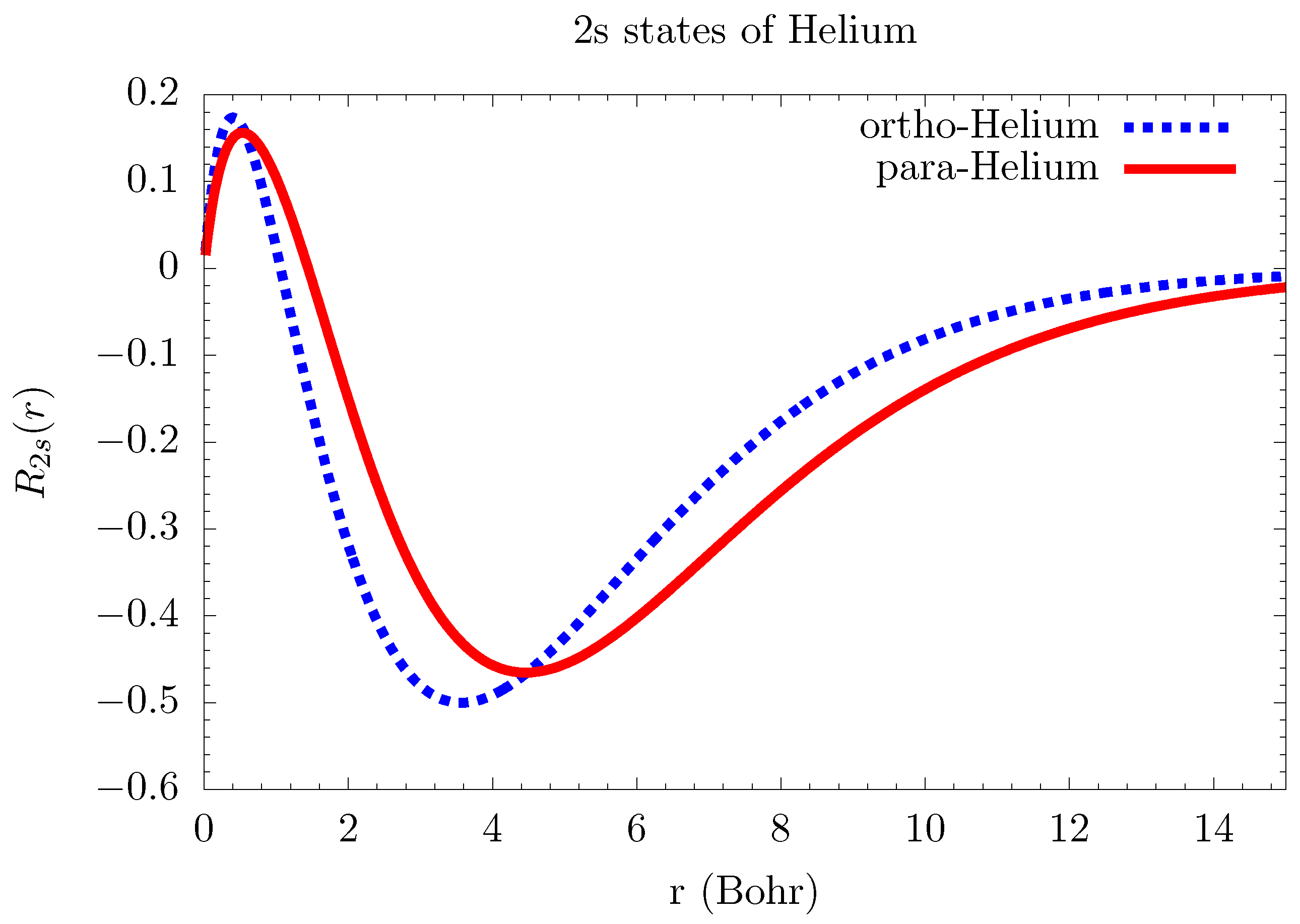
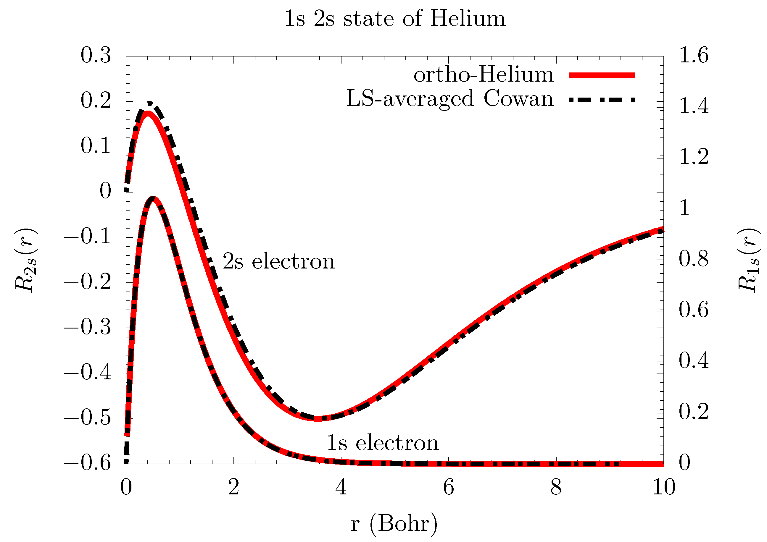
6.1. Atomic Structure

The changes in the atomic data will affect all spectral line shape calculations. All spectral line broadening calculations require input from an atomic structure code, and the most commonly-used information is the energy levels and dipole moments. As we showed in Section 4, the energy levels of the helium atom can substantially change with a different treatment of exchange. The small changes in the wavefunctions will also result in changes in the dipole moments used by line-shape codes.

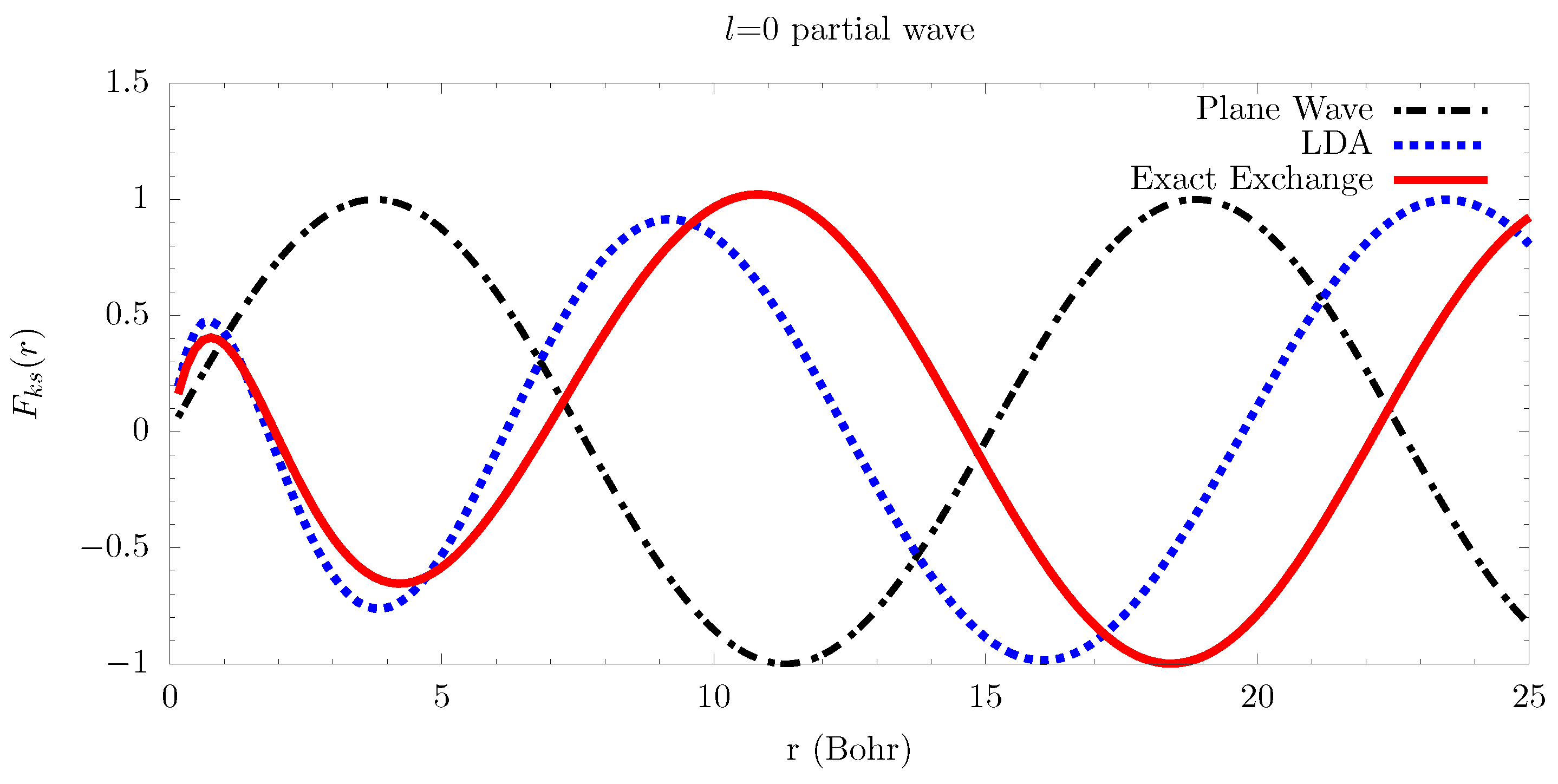
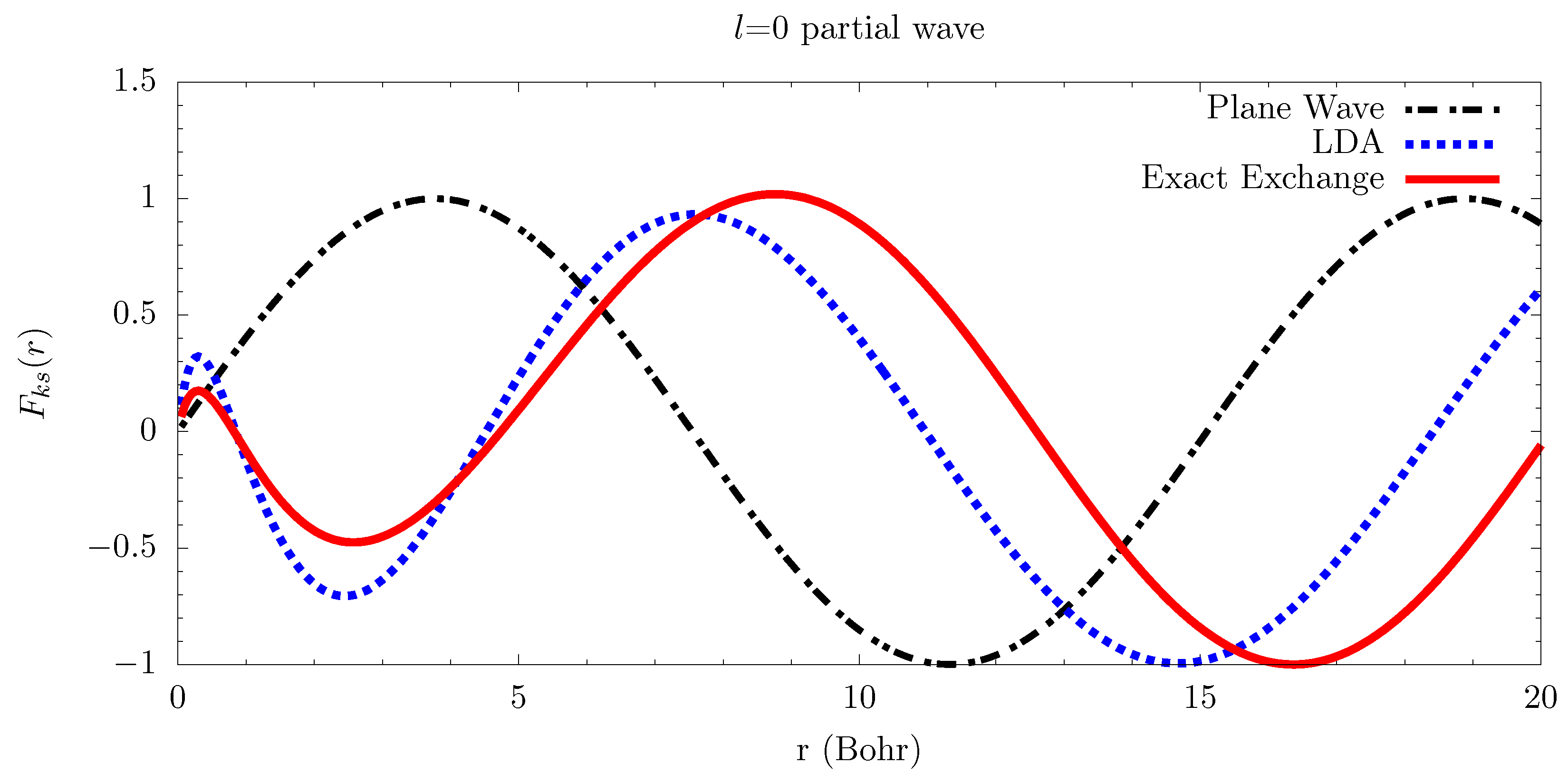
6.2. Electron-Atom Collisions

It has been well established that line broadening is closely related to collision amplitudes [15,37,38], therefore any discussion regarding collision amplitudes becomes important for line-broadening as well. Calculations of collision amplitudes, regardless of the method (second-order distorted-wave method [8,39], or a CCC method [4,15,40,41,42]), require a set of starting wavefunctions for the plasma electrons. Most of these methods use a LDA to approximate exchange, but as demonstrated in the previous sections, these may not be the most accurate when exchange becomes important5.

The choice of wavefunctions can have a significant impact on how the matrix elements required for electron collisions are calculated. For example, the exchange contribution (of a matrix element) is more complicated to calculate if the bound- and free-electron wavefunctions are not orthogonal, and become considerably simpler when the wavefunctions are orthogonal [21]. LDA methods do not guarantee orthogonality (giving overlap integrals up to 0.2), though it is commonly treated as approximately orthogonal6. The matrix method employed here provides overlap integrals that are less than 0.01 (and sometimes better than 0.001). However, there is a caveat here: while our wavefunctions are orthogonal to the bound electrons of the same configuration, they will not necessarily be orthogonal to bound electrons of a different configuration. In other words, free-electron wavefunctions calculated in the potential of the $1s^{2}2s$ state will not necessarily be orthogonal to the $1s^{2}3s$ electrons; this problem is common to both the LDA and matrix techniques. Due to these complications, we will only say (for now) that (by making the common assumption [21] that wavefunctions between configurations are orthogonal) the broadening of the $2s$→$2p$ transition of B iii can change by 10% by changing which wavefunctions are used.

Collision amplitudes can also be calculated by the difference in phase between Coulomb/plane waves and the wavefunction with the atomic interaction [7] (the broadening can be approximated as the difference in collision amplitudes of the upper- and lower-states of a given transition). Figure 3 and Figure 4 demonstrate that the LDA calculations give quite different phase shifts than the matrix method. This difference in phase shifts will not likely matter much for systems like hydrogen since the broadening of the upper state is usually much greater than the lower states. However, in multi-electron systems—specifically transitions where the principle quantum number does not change, such as the $1s^{2}2s$→$1s^{2}2p$ transition of lithium—the difference in LDA and matrix method wavefunctions can be significant. For all Li-like systems that we explored (neutral Li to Ne${}^{+7}$), the effective LDA potentials of the $1s^{2}2s$ and $1s^{2}2p$ are nearly identical and give identical phase shifts, which cancel for the calculation of electron broadening. However, using the matrix method results in different phase shifts between the $1s^{2}2s$ and $1s^{2}2p$ states, and will thus have a non-zero contribution to the broadening of the line.

7. Summary

We present a different technique for evaluating exchange effects in multi-electron atoms and in collision processes. Rather than treating the exchange term of the Hartree-Fock equations as an inhomogeneous term of the differential equation, we treat it explicitly as an integro-differential equation. We have written the exchange integral as a matrix and then, by approximating the rest of the Hamiltonian terms as finite-difference coefficients, we can use linear algebra packages such as LAPACK to diagonalize the total Hamiltonian to get the energies and wavefunctions. This method can be used for either bound-state, or free-state systems. These lead to some differences in the evaluation of the helium atom energy-level structure and wavefunctions. The behavior of penetrating free electrons near the origin is different from the LDA treatment of exchange for multi-electron systems, and can lead to changes in the broadening of theses systems.

References

1. Falcon, R.E.; Rochau, G.A.; Bailey, J.E.; Gomez, T.A.; Montgomery, M.H.; Winget, D.E.; Nagayama, T. Laboratory Measurements of White Dwarf Photospheric Spectral Lines: Hβ. Astrophys. J. 2015, 806, 214. [Google Scholar] [CrossRef]
2. Nagayama, T.; Bailey, J.E.; Mancini, R.C.; Iglesias, C.A.; Hansen, S.B.; Blancard, C.; Chung, H.K.; Colgan, J.; Cosse, P.; Faussurier, G.; et al. Model uncertainties of local-thermodynamic-equilibrium K-shell spectroscopy. High Energy Density Phys. 2016, 20, 17–22. [Google Scholar] [CrossRef]
3. Bergeron, P.; Saffer, R.A.; Liebert, J. A spectroscopic determination of the mass distribution of DA white dwarfs. Astrophys. J. 1992, 394, 228–247. [Google Scholar] [CrossRef]
4. Seaton, M.J. Atomic data for opacity calculations. XIII - Line profiles for transitions in hydrogenic ions. J. Phys. B 1990, 23, 3255–3296. [Google Scholar] [CrossRef]
5. Bethe, H.A.; Salpeter, E.E. Quantum Mechanics of One- and Two-Electron Atoms; Academic Press: New York, NY, USA, 1957. [Google Scholar]
6. Moiseiwitsch, B.L.; Smith, S.J. Electron Impact Excitation of Atoms. Rev. Mod. Phys. 1968, 40, 238–353. [Google Scholar] [CrossRef]
7. Mott, N.; Massey, H. The Theory of Atomic Collisions; The International Series of Monographs on Physics; Clarendon Press: London, UK, 1965. [Google Scholar]
8. Madison, D.H.; Bray, I.; McCarthy, I.E. Exact second-order distorted-wave calculation for hydrogen including second-order exchange. J. Phys. B 1991, 24, 3861–3888. [Google Scholar] [CrossRef]
9. Gomez, T.A. Improving Calculations of the Interaction Between Atoms and Plasma Particles and Its Effect on Spectral Line Shapes. Ph.D. Thesis, University of Texas at Austin, Austin, TX, USA, 2017. [Google Scholar]
10. Gunderson, M.A.; Junkel-Vives, G.C.; Hooper, C.F. A comparison of a second-order quantum mechanical and an all-order semi-classical electron broadening model. J. Quant. Spectrosc. Radiat. Transf. 2001, 71, 373–382. [Google Scholar] [CrossRef]
11. Alexiou, S.; Poquérusse, A. Standard line broadening impact theory for hydrogen including penetrating collisions. Phys. Rev. E 2005, 72, 046404. [Google Scholar] [CrossRef] [PubMed]
12. Gomez, T.A.; Nagayama, T.; Kilcrease, D.P.; Montgomery, M.H.; Winget, D.E. Effect of higher-order multipole moments on the Stark line shape. Phys. Rev. A 2016, 94, 022501. [Google Scholar] [CrossRef]
13. Woltz, L.A.; Hooper, C.F., Jr. Full Coulomb calculation of Stark broadening in laser-produced plasmas. Phys. Rev. A 1984, 30, 468–473. [Google Scholar] [CrossRef]
14. Junkel, G.C.; Gunderson, M.A.; Hooper, C.F., Jr.; Haynes, D.A., Jr. Full Coulomb calculation of Stark broadened spectra from multielectron ions: A focus on the dense plasma line shift. Phys. Rev. E 2000, 62, 5584–5593. [Google Scholar] [CrossRef]
15. Griem, H.R.; Ralchenko, Y.V.; Bray, I. Stark broadening of the B III 2s-2p lines. Phys. Rev. E 1997, 56, 7186–7192. [Google Scholar] [CrossRef]
16. Griem, H.R.; Ralchenko, Y.V. Electron collisional broadening of isolated lines from multiply-ionized atoms. J. Quant. Spec. Radiat. Transf. 2000, 65, 287–296. [Google Scholar] [CrossRef]
17. Ralchenko, Y.V.; Griem, H.R.; Bray, I. Electron-impact broadening of the 3s-3p lines in low-Z Li-like ions. J. Quant. Spec. Radiat. Transf. 2003, 81, 371–384. [Google Scholar] [CrossRef]
18. Glenzer, S.; Uzelac, N.I.; Kunze, H.J. Stark broadening of spectral lines along the isoelectronic sequence of Li. Phys. Rev. A 1992, 45, 8795–8802. [Google Scholar] [CrossRef] [PubMed]
19. Glenzer, S.; Kunze, H.J. Stark broadening of resonance transitions in B III. Phys. Rev. A 1996, 53, 2225–2229. [Google Scholar] [CrossRef] [PubMed]
20. Alexiou, S.; Dimitrijević, M.; Sahal-Brechot, S.; Stambulchik, E.; Duan, B.; González-Herrero, D.; Gigosos, M. The Second Workshop on Lineshape Code Comparison: Isolated Lines. Atoms 2014, 2, 157–177. [Google Scholar] [CrossRef]
21. Cowan, R.D. The Theory of Atomic Structure and Spectra; Los Alamos Series in Basic and Applied Sciences; University of California Press: Berkeley, CA, USA, 1981. [Google Scholar]
22. Fontes, C.J.; Zhang, H.L.; Jr, J.A.; Clark, R.E.H.; Kilcrease, D.P.; Colgan, J.; Cunningham, R.T.; Hakel, P.; Magee, N.H.; Sherrill, M.E. The Los Alamos suite of relativistic atomic physics codes. J. Phys. B 2015, 48, 144014. [Google Scholar] [CrossRef]
23. Hartree, D.R. The Wave Mechanics of an Atom with a Non-Coulomb Central Field. Part I. Theory and Methods. Proc. Camb. Philos. Soc. 1928, 24, 89. [Google Scholar] [CrossRef]
24. Fock, V. Näherungsmethode zur Lösung des quantenmechanischen Mehrkörperproblems. Z. Phys. 1930, 61, 126–148. [Google Scholar] [CrossRef]
25. Grant, I.P. Relativistic Quantum Theory of Atoms and Molecules; Springer Series on Atomic, Optical, and Plasma Physics; Springer Science+Business Media, LLC: Berlin, Germany, 2007; Volume 40, ISBN 978-0-387-34671-7. [Google Scholar]
26. Talman, J.D.; Shadwick, W.F. Optimized effective atomic central potential. Phys. Rev. A 1976, 14, 36–40. [Google Scholar] [CrossRef]
27. Shiozaki, T.; Hirata, S. Grid-based numerical Hartree-Fock solutions of polyatomic molecules. Phys. Rev. A 2007, 76, 040503. [Google Scholar] [CrossRef]
28. Beck, T.L. Real-space mesh techniques in density-functional theory. Rev. Mod. Phys. 2000, 72, 1041–1080. [Google Scholar] [CrossRef]
29. Chow, P.C. Computer Solutions to the Schrödinger Equation. Am. J. Phys. 1972, 40, 730–734. [Google Scholar] [CrossRef]
30. Pillai, M.; Goglio, J.; Walker, T.G. Matrix Numerov Method for solving Schrödinger’s equation. Am. J. Phys. 2012, 80, 1017–1019. [Google Scholar] [CrossRef]
31. Anderson, E.; Bai, Z.; Bischof, C.; Blackford, S.; Demmel, J.; Dongarra, J.; Du Croz, J.; Greenbaum, A.; Hammarling, S.; McKenney, A.; et al. LAPACK Users’ Guide; SIAM: Warrendale, PA, USA, 1999. [Google Scholar]
32. Sharma, C.S. On the Hartree-Fock equations for helium with non-orthogonal orbitals. J. Phys. B 1968, 1, 1023. [Google Scholar] [CrossRef]
33. Kramida, A.; Yu, R.; Reader, J.; NIST ASD Team. NIST Atomic Spectra Database (Ver. 5.5.2); National Institute of Standards and Technology: Gaithersburg, MD, USA, 2018. Available online: https://physics.nist.gov/asd (accessed on 16 April 2015).
34. Morton, D.C.; Wu, Q.X.; Drake, G.W.F. Energy levels for the stable isotopes of atomic helium (He-4 I and He-3 I). Can. J. Phys. 2006, 84, 83–105. [Google Scholar] [CrossRef]
35. Slater, J.C. A Simplification of the Hartree-Fock Method. Phys. Rev. 1951, 81, 385–390. [Google Scholar] [CrossRef]
36. Kohn, W.; Sham, L.J. Self-Consistent Equations Including Exchange and Correlation Effects. Phys. Rev. 1965, 140, 1133–1138. [Google Scholar] [CrossRef]
37. Baranger, M. General Impact Theory of Pressure Broadening. Phys. Rev. 1958, 112, 855–865. [Google Scholar] [CrossRef]
38. Fano, U. Pressure Broadening as a Prototype of Relaxation. Phys. Rev. 1963, 131, 259–268. [Google Scholar] [CrossRef]
39. Kingston, A.E.; Walters, H.R.J. Electron scattering by atomic hydrogen - The distorted-wave second Born approximation. J. Phys. B 1980, 13, 4633–4662. [Google Scholar] [CrossRef]
40. Bray, I. Convergent close-coupling method for the calculation of electron scattering on hydrogenlike targets. Phys. Rev. A 1994, 49, 1066–1082. [Google Scholar] [CrossRef] [PubMed]
41. Bray, I.; Stelbovics, A.T. Calculation of Electron Scattering on Hydrogenic Targets. Adv. Atom. Mol. Opt. Phys. 1995, 35, 209–254. [Google Scholar] [CrossRef]
42. Seaton, M.J.; Yan, Y.; Mihalas, D.; Pradhan, A.K. Opacities for Stellar Envelopes. Mon. Not. R. Astron. Soc. 1994, 266, 805. [Google Scholar] [CrossRef]
43. Gomez, T.A.; Nagayama, T.; Kilcrease, D.P.; Fontes, C.J.; Hansen, S.B.; Montgomery, M.H.; Winget, D.E. Penetrating Collisions by Electrons and its Effect on Electron Broadening. 2018; in preparation. [Google Scholar]
44. Fourth SLSP Workshop, In Proceedings of the Fourth Spectral Line Shape in Plasmas Code Comparison Workshop, Baden, Austria, 20–24 March 2017. Available online: http://plasma-gate.weizmann.ac.il/projects/slsp/slsp4/ (accessed on 20 March 2018).
1
Current calculations [15,16,17] that include electron exchange, however, are unable to match the measured broadening of these lines [18,19]; the reason for this discrepancy is unknown. This is the long-standing isolated-line problem, see Alexiou et al. [20] for a review.
2
This method fails to capture some correlation effects because the potential in which the electron is moving is defined to be a mean field of the other electrons, which is to say that it does not account for the strong repulsion when the two electrons are close to each other.
3
If the two wavefunctions are assumed to be orthogonal, then these terms vanish.
4
In fact, radial solutions of three-electron problems can be solved on a laptop with the help of sparse matrix eigenvalue solvers. Any system larger than this would require the use of a supercomputer.
5
This method of using an exact exchange treatment is now being implemented in the DWE line shape code [9,43] (which was used in the SLSP4 workshop [44]), which improves upon the relaxation theory method of Junkel et al. [14] to include exchange.
6
This may be a dangerous approximation because some (non-negligible) processes need to be considered when orthogonality is not guaranteed.
Figure 1. Numerical results of using matrix exchange method.
Atoms 06 00022 g001
Figure 2. The ortho-helium wavefunctions compared with Cowan’s 1s 2s wavefunction. The new calculations with exact exchange are given in red, while Cowan’ calculation are in dot-dashed black lines.
Atoms 06 00022 g002
Figure 3. The l = 0 partial wave of the free-electron wavefunction under different approximations. Black dot dashed is the plane wave, dotted blue is using an LDA to approximate the exchange correlations, and solid red is the exact exchange treatment. The states are reacting to the presence of a hydrogen atom in the 2 s state.
Atoms 06 00022 g003
Figure 4. Same as Figure 3, but reacting to the Li 1 s 2 2 s state.
Atoms 06 00022 g004