Hybrid Theory of Scattering and Its Applications

Abstract

A number of formulations have been used to investigate scattering of low-energy electrons and positrons from various targets. The hybrid theory of scattering, which takes into account the short-range as well as the long-range correlations, and is variationally correct, is described in this article. This approach has been applied to calculate phase shifts for scattering of electrons and positrons, resonances in two-electron systems, photodetachment, and photoionization of two-electron systems. This approach has also been applied to calculate excitation of 2s state of atomic hydrogen by electron impact. In photoabsorption the target can be left in 2p state instead of 1s state, resulting in the emission of Lyman-alpha radiation. Cross sections for this process are also calculated.

1. Introduction and Calculations

Scattering by single-electron systems is always of interest because the wave function of the target is known exactly. Also, scattering from atoms helps us to understand their static and dynamic properties. It also has applications in astrophysics and in the investigation of controlled thermonuclear devices. Different approaches have been applied to study scattering of electrons and positrons from various targets, to infer the feasibility of various calculations and the accuracy of their results. In other words, this is an ideal problem for testing various theories. A simple method is to assume that the wave function of the incident electron on hydrogen atom is given by $\mathsf{\Psi }({\overrightarrow{r}}_1,{\overrightarrow{r}}_2)=u({\overrightarrow{r}}_1){\mathsf{\Phi }}_0({\overrightarrow{r}}_2)$, where ${\mathsf{\Phi }}_0({\overrightarrow{r}}_2)$ is the ground state of the hydrogen atom and $u({\overrightarrow{r}}_1)$ is the function whose asymptotic limit determines phase shift of the scattering. Morse and Allis [1] introduced exchange between electrons, writing the wave function in the form:

$$\mathsf{\Psi }({\overrightarrow{r}}_1,{\overrightarrow{r}}_2)=u({\overrightarrow{r}}_1){\mathsf{\Phi }}_0({\overrightarrow{r}}_2)\pm u({\overrightarrow{r}}_2){\mathsf{\Phi }}_0({\overrightarrow{r}}_1).$$

(1)

The ground state function is given by:

$${\mathsf{\Phi }}_0({\overrightarrow{r}}_2)=\sqrt{\frac{Z^3}{\pi }}{e}^{-Z{r}_2}.$$

(2)

The upper sign in Equation (1) corresponds to the singlet state and the lower sign corresponds to triplet state of the system. The equation for the scattering function u(r) (letting r₁ = r) is obtained by the Kohn variation of the functional:

$$\langle Y_{L0}({\Delta }_1){\mathsf{\Phi }}_0({\overrightarrow{r}}_2)|H-E|\mathsf{\Psi }({\overrightarrow{r}}_1,{\overrightarrow{r}}_2)\rangle =0,$$

(3)

where E = k² − Z² and k² is the kinetic energy of the incident electron, and Z is the charge of the nucleus. Considering the proton stationary during the interaction, the Hamiltonian H of the system in Rydberg units is given by:

$$H=-{\nabla }_1^2-{\nabla }_2^2-\frac{2Z}{r_1}-\frac{2Z}{r_2}+\frac{2}{r_{12}}$$

(4)

In the above equation, $r_{12}=|{\overrightarrow{r}}_1-{\overrightarrow{r}}_2|$. Using Equation (3), we get the integro-differential equation:

$$\begin{gathered} [\frac{d^2}{d{r}^2}+\frac{2(Z-1)}{r}-\frac{L(L+1)}{r}+e^{-2Zr}2(Z+\frac{1}{r})+k^2)]u(r)\pm 4Z^3{e}^{-Zr}[(k^2+Z^2)r{\delta }_{L0}{I}_1 \\ -\frac{2}{2L+1}(\frac{I_2}{r^L}+r^{L+1}{I}_3)]=0. \end{gathered}$$

(5)

The exchange terms with $I_1$, $I_2$, and $I_3$ are the nonlocal potentials and are functions of u(r):

$$I_1={\displaystyle \underset{0}{\overset{\infty }{\int }}{e}^{-Zx}xu(x)dx},$$

(6)

$$I_2={\displaystyle \underset{0}{\overset{r}{\int }}{e}^{-Zx}{x}^{L+1}u(x)dx},$$

(7)

and

$$I_3={\displaystyle \underset{r}{\overset{\infty }{\int }}{e}^{-Zx}\frac{u(x)}{x^L}dx}.$$

(8)

The singlet and triplet S-wave phase shifts in the exchange approximation are given in

Table 1. Phase shifts (radians) for the ¹S and ³S states of e-H.

K	Singlet			Triplet
	EAa	PO [6]	QHQ [7]	EAa	PO [6]	QHQ [7]
0.0	8.100	5.9		2.349	1.9
0.1	2.396	2.583	2.55358	2.908	2.945	2.93853
0.2	1.870	2.144	2.06678	2.679	2.732	2.71741
0.3	1.508	1.750	1.69816	2.461	2.519	2.49975
0.4	1.239	1.469	1.41540	2.257	2.320	2.29408
0.5	1.031	1.251	1.20094	2.070	2.133	2.10454
0.6	0.869		1.04083	1.901		1.93272
0.7	0.744	0.947	0.93111	1.749	1.815	1.77950
0.8	0.651	0.854	0.88718	1.614	1.682	1.64379

EA^a are exchange approximation phase shifts, and k = 0 results are scattering lengths.

. Among the different methods used is the variational principle of Kohn [2]. Schwartz [3] used this principle to calculate phase shifts of electrons and positrons scattering from hydrogen atoms. There are no bounds on phase shifts in this principle except at incident energy k = 0. There are also singularities in this calculation. In spite of singularities, the results obtained in [3] are fairly accurate and have stood the test of time. Another extensively used method is the close-coupling approximation [4], in which the total wave function is expanded in eigenstates of the hydrogen atom. Accurate results have been obtained using the R-matrix formulation [5] in which most of the complications of interactions are taken into account within the inner region of a certain radius and outside this radius plane waves or Coulomb waves are used for continuum functions.

It has been emphasized by Wigner [8] that long range forces determine the nature of the scattering parameters at threshold. A method in which the longest-range potential proportional to −1/r⁴ is taken into account is the method of polarized orbital [6,9]. This method includes the essential physics of the problem and has been widely used not only to calculate scattering parameters for electrons and positrons but also to calculate photoabsorption cross sections. Using the first-order perturbation theory and the dipole part of the perturbed wave function, Temkin [9] showed that the effective target wave function in the presence of the incident electron can be written as

$${\mathsf{\Phi }}^{pol}({\overrightarrow{r}}_1,{\overrightarrow{r}}_2)={\mathsf{\Phi }}_0({\overrightarrow{r}}_2)-\frac{\epsilon (r_1,r_2)}{r_1^2}\frac{u_{1s\to p}(r_2)}{r_2}\frac{\cos ({\theta }_{12})}{\sqrt{Z\pi }}$$

(9)

where

$$u_{1s\to p}(r_2)=e^{-Z{r}_2}(0.5Z{r}_2^3+r_2^2).$$

(10)

$$\begin{gathered} \epsilon (r_1,r_2)=1,r_1>r_2 \\ =0,r_1<r_2. \end{gathered}$$

(11)

Now, the function in Equation (1) is written as:

$$\mathsf{\Psi }({\overrightarrow{r}}_1,{\overrightarrow{r}}_2)=u({\overrightarrow{r}}_1){\mathsf{\Phi }}^{pol}({\overrightarrow{r}}_1,{\overrightarrow{r}}_2)\pm (1\leftrightarrow 2).$$

(12)

The equation for the scattering function $u_L(r_1)$ can be derived from:

$$\langle Y_{L0}({\Delta }_1){\mathsf{\Phi }}_0(r_2)|H-E|\mathsf{\Psi }({\overrightarrow{r}}_1,{\overrightarrow{r}}_2)\rangle =0$$

(13)

The equation for the scattering function $u_L(r)$ for all momenta has been given by Sloan [10]:

$$\begin{array}{l}[\frac{d^2}{d{r}^2}+\frac{2(Z-1)}{r}-\frac{L(L+1)}{r}+e^{-2Zr}2(Z+\frac{1}{r})+k^2)]u_L(r)\pm 4Z^3{e}^{-Zr}[(k^2+Z^2)r{\delta }_{L0}{I}_1\\ \hspace{1em}\hspace{1em}\hspace{1em}\hspace{1em}-\frac{2}{2L+1}\{r^{-L}{I}_2+r^{L+1}{I}_3\}]=-\frac{\alpha (Zr)}{{(Zr)}^4}{u}_L(r)\\ \hspace{1em}\hspace{1em}\hspace{1em}\hspace{1em}\mp 4Z{e}^{-Zr}[\frac{{\delta }_{L1}}{3}\{-\frac{Z(Z^2+k^2)}{2}{r}^3+(Z^2-k^2)r^2\}{\displaystyle \underset{r}{\overset{\infty }{\int }}{e}^{-Zx}{x}^{-L}{u}_L(x)dx}\\ \hspace{1em}\hspace{1em}\hspace{1em}\hspace{1em}+2(Z{r}^3+r^2)\{\frac{L}{(2L-1)(2L+1)}{r}^{L-1}{\displaystyle \underset{r}{\overset{\infty }{\int }}{e}^{-Zx}{x}^{-L-1}{u}_L(x)dx}\\ \hspace{1em}\hspace{1em}\hspace{1em}\hspace{1em}+\frac{L+1}{(2L+1)(2L+3)}{r}^{L+1}{\displaystyle \underset{r}{\overset{\infty }{\int }}{e}^{-Zx}{x}^{-L-3}{u}_L(x)dx}\}]\\ \hspace{1em}\hspace{1em}\hspace{1em}\hspace{1em}\pm \frac{4}{3}{\delta }_{L1}{e}^{-2Zr}[(\frac{3}{2}{Z}^2{r}^2+\frac{1}{2}Zr-3)u_L(r)-(\frac{1}{2}Z{r}^2+r)\frac{d{u}_L(r)}{dr}],\end{array}$$

(14)

where

$$\alpha (x)=\frac{9}{2}-\frac{2}{3}{e}^{-2x}(x^5+\frac{9}{2}{x}^4+9x^3+\frac{27}{2}{x}^2+\frac{27}{2}x+\frac{27}{4}).$$

(15)

The scattering equation has the well-known attractive potential which for large r is equal to $-\alpha /{(Zr)}^4$, α = 4.5 $a_0^3$ being the asymptotic polarizability for a hydrogen atom. Temkin and Lamkin [6], using this method of polarized orbitals, calculated S-wave phase shifts, as well as for higher partial waves, for scattering of an electron from a hydrogen atom. Phase shifts are determined by the asymptotic limit of the function $u_L(r)$:

$$\underset{r\to \infty }{\lim }{u}_L(r)=\frac{\sin (kr-\pi L/2+{\sigma }_C+\eta )}{r}.$$

(16)

The Coulomb phase in the above equation is given by:

$${\sigma }_C=\frac{Z-1}{k}\ln (2kr)+\arg \Gamma (L+1-\frac{i(Z-1)}{k}).$$

(17)

S-wave phase shift obtained by this method are given in Table 1 and they differ from those obtained in the exchange approximation, showing the importance of polarization of the target resulting in the long-range potential −1/r⁴. However, this method does not provide variational bounds to the exact phase shifts.

The short-range correlations can be important in addition to the long-range correlations. These short-range correlations can be included using the projection-operator formalism of Feshbach [11]:

P = P₁ + P₂ − P₁P₂.  and    Q = 1 − P.

(18)

The wave function in Equation (1) is augmented by a correlation function${\mathsf{\Phi }}_L({\overrightarrow{r}}_1,{\overrightarrow{r}}_2)$:

$$\mathsf{\Psi }({\overrightarrow{r}}_1,{\overrightarrow{r}}_2)=u({\overrightarrow{r}}_1){\mathsf{\Phi }}_0({\overrightarrow{r}}_2)\pm (1\leftrightarrow 2)+{\mathsf{\Phi }}_L({\overrightarrow{r}}_1,{\overrightarrow{r}}_2)$$

(19)

where

$${\mathsf{\Phi }}_L({\overrightarrow{r}}_1,{\overrightarrow{r}}_2)={\displaystyle \sum \{f_L^{\kappa ,1}(r_1,r_2,r_{12})D_L^{\kappa ,1}(\theta ,\varphi ,\psi )+f_L^{\kappa ,-1}(r_1,r_2,r_{12})D_L^{\kappa ,-1}(\theta ,\varphi ,\psi )\}.}$$

(20)

The radial functions are of Hylleraas type and D’s are rotational harmonics [12].

The projections are defined by:

$$P_1\mathsf{\Phi }({\overrightarrow{r}}_1,{\overrightarrow{r}}_2)={\mathsf{\Phi }}_0({\overrightarrow{r}}_1){\displaystyle \int {\mathsf{\Phi }}_0({\overrightarrow{r}}_1){\mathsf{\Phi }}_L({\overrightarrow{r}}_1,{\overrightarrow{r}}_2)d{\overline{r}}_1}.$$

(21a)

$$P_2\mathsf{\Phi }({\overrightarrow{r}}_1,{\overrightarrow{r}}_2)={\mathsf{\Phi }}_0({\overrightarrow{r}}_2){\displaystyle \int {\mathsf{\Phi }}_0({\overrightarrow{r}}_2){\mathsf{\Phi }}_L({\overrightarrow{r}}_1,{\overrightarrow{r}}_2)d{\overrightarrow{r}}_2}.$$

(21b)

Using the projection operators P and Q, we get the equation for the scattering function $u_L^{(\pm )}(r)$, having an optical potential [7]. The equation for the scattering function $u_L^{(\pm )}(r)$ is given by the following equation:

$$[-\frac{d^2}{d{r}^2}+\frac{L(L+1)}{r^2}+V_d\pm V_{ex}+V^{(\pm )}{}_{op}(P,Q)-k^2]u_L^{(\pm })(r)=0$$

(22)

where $V_d$ and $V_{ex}$ are the direct and nonlocal exchange potentials of the ‘exchange approximation’ [1]. $V_{op}^{(\pm )}(P,Q)$ is the optical potential which is negative definite and therefore attractive. The optical potential acting on $u_L(r)$ is given by:

$$V_{op}^{(\pm )}(P,Q)u_L=r\langle Y_{L0}PHQ\frac{1}{E-QHQ}QHP{\mathsf{\Psi }}_L\rangle .$$

(23)

We find S-wave phase shifts, given in Table 1, increase compared to the exchange approximation when short-range correlations are included but not the long-range correlations at the same time. However, the phase shifts obtained by this method have lower bounds to the exact phase shifts.

Is it possible to consider the long-range and short-range correlations at the same time? The projection-operator formalism, when both type of correlations are included, does not work because it is not possible to construct projection operators when ${\mathsf{\Phi }}^{pol}({\overrightarrow{r}}_1,{\overrightarrow{r}}_2)$ instead of ${\mathsf{\Phi }}_0({\overrightarrow{r}}_2)$ is used in the definitions given in Equation (21). However, we can write a wave function which has a long-range and a short-range parts at the same time and we call this formulation hybrid theory because it includes both type of correlations: short-range as well as long-range at the same time. We describe this formalism by confining ourselves to the e-H partial wave (denoted by L) problem. The total spatial wave function is written as:

$${\mathsf{\Psi }}_L({\overrightarrow{r}}_1,{\overrightarrow{r}}_2)=\frac{u_L(r_1)}{r_1}{Y}_{L0}({\Delta }_1){\mathsf{\Phi }}^{pol}({\overrightarrow{r}}_1,{\overrightarrow{r}}_2)\pm (1\leftrightarrow 2)+{\displaystyle \sum _{\lambda =1}^N{C}_{\lambda }}{\mathsf{\Phi }}_L^{\lambda }({\overrightarrow{r}}_1,{\overrightarrow{r}}_2).$$

(24)

The functions ${\mathsf{\Phi }}^{pol}({\overrightarrow{r}}_1,{\overrightarrow{r}}_2)$ and ${\mathsf{\Phi }}_L({\overrightarrow{r}}_1,{\overrightarrow{r}}_2)$ are given in Equations (9) and (20), respectively. This approach is variationally correct and phase shifts obtained have lower bounds to the exact phase shifts. This has been achieved by introducing separate correlation functions and then amalgamating them into the scattering problem, via an optical potential, in order to replace the many-particle Schrödinger equation with a single-particle Schrödinger equation.

We can derive the equation for the scattering function u(r) from (letting r₁ = r) from the functional:

$$I=\langle {\mathsf{\Psi }}_L({\overrightarrow{r}}_1,{\overrightarrow{r}}_2)|H-E|{\mathsf{\Psi }}_L({\overrightarrow{r}}_1,{\overrightarrow{r}}_2)\rangle =0.$$

(25)

For S-waves, we can write:

$${\mathsf{\Phi }}_{L=0}({\overrightarrow{r}}_1,{\overrightarrow{r}}_2)=\sum _{lmn}^{N_{\omega }}{C}_{lmn}[e^{-\gamma r_1-\delta r_2}{r}_1^l{r}_2^m{r}_{12}^n\pm (1\leftrightarrow 2)]$$

(26)

C_lmn in Equation (26) are coefficients which are determined when eigenvalues are calculated using the Ritz variational principle. For $N_{\omega }$ = 1, the functional can be written as:

$$I=A+C_{1}B+{C_1}^{2}D.$$

(27)

where

$$A=\langle [{\mathsf{\Phi }}^{pol}u({\overrightarrow{r}}_1)\pm (1\to 2)]|H-E|[{\mathsf{\Phi }}^{pol}u({\overrightarrow{r}}_1)\pm (1\to 2)]\rangle$$

(28)

and

$$\begin{array}{l}B=2\langle {\mathsf{\Phi }}_L^1({\overrightarrow{r}}_1,{\overrightarrow{r}}_2)|H-E|[{\mathsf{\Phi }}^{pol}u({\overrightarrow{r}}_1)\pm (1\to 2)]\rangle \\ =4\langle V_1({\overrightarrow{r}}_1)u({\overrightarrow{r}}_1)\rangle .\end{array}$$

(29)

We can determine C₁ by:

$$\frac{dI}{d{C}_1}=0.$$

(30)

which implies that:

$$B+2C_{1}D=0$$

(31)

This gives

$$C_1=-B/2D=\frac{2\langle V_1({\overrightarrow{r}}_1)u({\overrightarrow{r}}_1)\rangle }{E-{\epsilon }_1}.$$

(32)

where

$$V_1(r_1)=\langle {\mathsf{\Phi }}_L^{(1)}({\overrightarrow{r}}_1,{\overrightarrow{r}}_2)|H-E|{\mathsf{\Phi }}^{pol})\rangle ,$$

(33)

$$D=\langle {\mathsf{\Phi }}_L^{(1)}|H-E|{\mathsf{\Phi }}_L^{(1)}\rangle ={\epsilon }_1-E.$$

(34)

We can generalize the above treatment to any number of unknown coefficients in Equation (24). Now all the quantities in Equation (24) are known except $u_L(r)$. The equation for the scattering function $u_L(r)$ can be derived from:

$$\langle Y_{L0}({\Delta }_1){\mathsf{\Phi }}^{pol}|H-E|\mathsf{\Psi }({\overrightarrow{r}}_1,{\overrightarrow{r}}_2)\rangle =0.$$

(35)

The resulting equation is fairly complicated and the various quantities are given in [13]. We give a few of them below. We can generalize the above treatment to any number of unknown coefficients in Equation (24). We write the wave function in the form:

$${\mathsf{\Psi }}_L({\overrightarrow{r}}_1,{\overrightarrow{r}}_2)=u_L({\overrightarrow{r}}_1){\mathsf{\Phi }}^{pol}({\overrightarrow{r}}_1,{\overrightarrow{r}}_2)\pm (1\leftrightarrow 2)+{\displaystyle \sum _{\lambda }{C}_{\lambda }{\mathsf{\Phi }}_L^{\lambda }({\overrightarrow{r}}_1,{\overrightarrow{r}}_2)}.$$

(36)

We define now:

$${\mathsf{\Phi }}^{pol}({\overrightarrow{r}}_1,{\overrightarrow{r}}_2)={\mathsf{\Phi }}_0({\overrightarrow{r}}_2)-\frac{{\chi }_{\beta }(r_1)}{r_1^2}\frac{u_{1s\to p}(r_2)}{r_2}\frac{\cos ({\theta }_{12})}{\sqrt{\pi Z}}.$$

(37)

We have replaced the step function $\epsilon (r_1,r_2)$ by:

$${\chi }_{\beta }(r_1)={(1-e^{-\beta r_1})}^n.$$

(38)

The exponent n is found to be 3 or 4. Now, polarization takes place for any value of r₁, the coordinate of the incident electron. In the method of polarized orbitals, the orbital of the target was perturbed only when the incident electron was outside the target. Now perturbation takes place whether the incident electron is outside or inside of the target.

In addition to the nonlinear parameters in the correlation function, β is another nonlinear parameter and it is a function of the incident momentum k. This further helps in getting improved results. There is another form of the smooth cutoff function given by Shertzer and Temkin [14]:

$${\chi }_{ST}(r_1)=1-e^{-2Z{r}_1}(\frac{1}{3}{(Z{r}_1)}^4+\frac{4}{3}{(Z{r}_1)}^3+2{(Z{r}_1)}^2+2Z{r}_1+1).$$

(39)

All the quantities are now known in the wave function given in Equation (24). We can derive the equation for the scattering function using Equation (35). The equation for the scattering function is again is of the same form as Equation (22), but with more terms:

$$[D(r)\frac{d^2}{d{r}^2}-\frac{L(L+1)}{r^2}+V_d+V_d^{pol}\pm (V_{ex}+V_{ex}^{pol})-V_{op}^{pol}+k^2]u(r)=0.$$

(40)

As stated earlier, most of the quantities are given in [13]. Some of these quantities occurring in the direct potential are given below:

$$D(r)=1+\frac{43}{8Z^6}{(\frac{\chi (r)}{r^2})}^2.$$

(41)

The direct potentials are given by:

$$V_d=\frac{2(Z-1)}{r}+2e^{-Zr}(Z+\frac{1}{r}).$$

(42a)

We repeat here the exchange terms already indicated in Equation (5):

$$V_{ex}{u}_L(r)=4Z^3{e}^{-Zr}\{(k^2+Z^2)r{\delta }_{L0}{I}_1-\frac{2}{2L+1}(\frac{I_2}{r^{L+1}}+r^{L+1}{I}_3)\}$$

(42b)

$$V_d^{pol}=(x_1+x_2)+x_3\frac{d}{dr}.$$

(43)

$$x_1=\frac{43}{8Z^6}(\frac{2Z}{r}-\frac{2}{r^2}+k^2){(\frac{\chi (r)}{r^2})}^2.$$

(44)

$$x_2=B_1(r)\frac{43}{8Z^6}(\frac{\chi (r)}{r^2}).$$

(45)

$$x_3=B_2(r)\frac{43}{8Z^6}(\frac{\chi (r)}{r^2})+\frac{2\alpha (r)}{{(Zr)}^4}\chi (r)-\frac{9}{2}\frac{\chi {(r)}^2}{{(Zr)}^4}-\frac{8}{3Z}d(r){(\frac{\chi (r)}{r^2})}^2,$$

(46)

$$B_1(r)=\frac{1}{r^2}[-2Z\chi (r)+2Z-\frac{2}{r}+e^{-2Zr}(-\frac{2}{3}{Z}^4{r}^3-\frac{4}{3}{Z}^3{r}^2+2Z+\frac{2}{r})],$$

(47)

$$B_2(r)=-2Z{B}_1(r)-\frac{4Z}{r^3}+\frac{6}{r^4}+e^{-2Zr}(\frac{4}{3}{Z}^{5}r+2Z^4-\frac{4Z^2}{r^2}-\frac{8Z}{r^3}-\frac{6}{r^4}).$$

(48)

$$\alpha (r)=\frac{9}{2}-\frac{2}{3}{e}^{-2Zr}(\frac{3}{2}{(Zr)}^4+\frac{15}{2}{(Zr)}^3+\frac{27}{2}{(Zr)}^2+\frac{27}{2}(Zr)+\frac{27}{4}).$$

(49)

The last term in $x_3$ has:

$$\begin{array}{c}d(r)=\frac{129}{32Z^5}\frac{1}{r}+\frac{18}{Z^7}\frac{1}{r^3}-e^{-2Zr}(\frac{3}{16}{r}^4+\frac{27}{16Z}{r}^3+\frac{54}{8Z^2}{r}^2+\frac{135}{8Z^3}r\\ +\frac{975}{32Z^4}+\frac{1281}{32Z^5}\frac{1}{r}+\frac{36}{Z^6}\frac{1}{r^2}+\frac{18}{Z^7}\frac{1}{r^3})\end{array}$$

(50)

For $r\to \infty$, $x_3$ has a term

$$\frac{9}{2Z^4}$$

(51)

which is the dipole polarizability of the target with nuclear charge Z. $V_{op}^{pol}$ = optical potential which is attractive, but does not depend on projection operators, and is given by:

$$V_{op}^{pol}{u}_L(r_1)=r_1{\displaystyle \sum _s^{N_{\omega }}\frac{\langle Y_{L0}{\Delta }_1){\mathsf{\Phi }}^{pol}({\overrightarrow{r}}_1,{\overrightarrow{r}}_2)|H-E|{\mathsf{\Phi }}_L^s\rangle \langle {\mathsf{\Phi }}_L^s|H-E|{\mathsf{\Psi }}_L^{\text{'}}\rangle }{E-{\epsilon }_s}}.$$

(52)

The function ${\mathsf{\Psi }}_L^{\prime }$ is the function given in Equation (24) without the correlation terms. Phase shifts, given in

Table 2. Comparison of phase shifts (radians) obtained in hybrid theory [13] with those obtained by Schwartz [3] and Scholz et al. [15], the results for k = 0 are scattering lengths.

k	Singlet			Triplet
	${\mathit{\eta }}_{\mathit{H}\mathit{B}}$ [13]	${\mathit{\eta }}_{\mathit{s}\mathit{c}\mathit{h}\mathit{w}\mathit{a}\mathit{r}\mathit{t}\mathit{z}}$ [3]	${\mathit{\eta }}_{\mathit{S}\mathit{S}\mathit{B}}$ [15]	${\mathit{\eta }}_{\mathit{H}\mathit{B}}$ [13]	${\mathit{\eta }}_{\mathit{S}\mathit{c}\mathit{h}\mathit{w}\mathit{a}\mathit{r}\mathit{t}\mathit{z}}$ [3]	${\mathit{\eta }}_{\mathit{S}\mathit{S}\mathit{B}}$ [15]
0.0	5.99567	5.965		1.78154	1.7686
0.1	2.55370	2.553	2.550	2.93856	2.9388	2.939
0.2	2.06717	2.0673	2.062	2.71751	2.7171	2.717
0.3	1.69684	1.6964	1.691	2.49987	2.4996	2.500
0.4	1.41554	1.4146	1.410	2.29457	2.2938	2.294
0.5	1.20195	1.202	1.196	2.10574	2.1046	2.105
0.6	1.04191	1.041	1.035	1.93336	1.9329	1.933
0.7	0.93084	0.930	0.925	1.77999	1.7797	1.780
0.8	0.88802	0.886		1.64444	1.643

, are calculated using the asymptotic limit of the function $u_L(r)$ given in Equation (16).

We see that the method of polarized orbitals over estimates phase shifts. In the variational formulation, phase shifts have lower bounds to the exact phase shifts, that is, they can be higher than those given in Table 2 when the number of correlations terms in Equation (24) is increased. The phase shifts obtained using hybrid theory agree well with those obtained by Schwartz [3] and also with those obtained by Scholz et al. [15] using the close-coupling approximation. Similar calculations have been carried out for S-wave electron scattering from He⁺ and Li²⁺ [16]. These results are shown in

Table 3. Phase shifts (radians) for scattering of electrons from He⁺ and Li²⁺ [16].

k	He+		Li2+
	1S	3S	1S	3S
0.1	0.43808	0.93065	0.23188	0.56084
0.2	0.43550	0.92704	0.23176	0.56020
0.3	0.43142	0.92114	0.23148	0.55869
0.4	0.42608	0.91302	0.23109	0.55678
0.5	0.41974	0.90282	0.23064	0.55435
0.6	0.41265	0.89057	0.23012	0.55142
0.7	0.40568	0.87645	0.22960	0.54799
0.8	0.39865	0.86066	0.22906	0.54413
0.9	0.39123	0.84366	0/22855	0.53925
1.0	0.38644	0.82536	0.22807	0.53514
1.1	0.38200	0.80636	0.22769	0.53000
1.2	0.37914	0.78677	0.22740	0.52456
1.3	0.37846	0.76696	0.22724	0.51880
1.4	0.38158	0.74708	0.22724	0.51276
1.5	0.39802	0.72746	0.22742	0.50646
1.6	0.34480	0.70815	0.22782	049997

and they agree with those obtained by Gien [17,18] using the Harris-Nesbet variational method.

Calculations have been carried out for partial wave L = 1 for electron scattering from H, He⁺, and Li²⁺ [19,20]. The P-wave phase shifts for electron-H scattering are given in

Table 4. P-wave phase shifts (radians) for electron-hydrogen scattering. ${\eta }_{HB}$ are the results obtained using hybrid theory [19], ${\eta }_{RM}$ are the R-matrix results [15], and ${\eta }_{FEM}$ are finite-element method results [21].

K	1P			3P
	${\mathit{\eta }}_{\mathit{H}{\mathit{B}}^{}}$	${\mathit{\eta }}_{\mathit{R}\mathit{M}}$	${\mathit{\eta }}_{\mathit{F}\mathit{E}\mathit{M}}$	${\mathit{\eta }}_{\mathit{H}\mathit{B}}$	${\mathit{\eta }}_{\mathit{R}\mathit{M}}$	${\mathit{\eta }}_{\mathit{F}\mathit{E}\mathit{M}}$
0.1	0.00635076	0.006	0.006	0.01038234	0.010	0.0100
0.2	0.01506556	0.015	0.0148	0.04536735	0.045	0.0452
0.3	0.01670634	0.016	0.0160	0.1069312	0.107	0.1067
0.4	0.01015347	0.009	0.0090	0.1888873	0.187	0.1873
0.5	−0.00061223	−0.002	−0.0020	0.2709762	0.270	0.2708
0.6	−0.01009367	−0.012	−0.0117	0.3416749	0.341	0.3417
0.7	−0.01321557	−0.016	−0.0149	0.3932100	0.392	0.3933
0.8	−0.0046818		−0.0068	0.4277296		0.4283

. They are compared with those obtained using the R-matrix method [15] and by the finite-element method [21]. We see that the singlet P phase shifts have a peak at k = 0.3, while the triplet P phase shifts increase continuously.

Calculations have also been carried for partial wave L = 2 for electron scattering from H, He⁺, and Li²⁺ and photoabsorption when the final state is a 2p state [22].

2. Scattering Length

The scattering length a (in units of Bohr radius$a_0$) is defined by:

$$\underset{k\to 0}{{\displaystyle \lim }}k\cot (\eta )=-1/a.$$

(53)

Temkin [23] has shown that the scattering length is significantly affected by the long-range polarization potential. It is given by:

$$a=a(R)-\alpha (\frac{1}{R}-\frac{a}{R^2}+\frac{a^2}{3R^3})$$

(54)

where α is the fine structure constant.

For ¹S, for $N_{\omega }$ = 70 we find a(R) = 6.00239 at R = 117.3038, using the above correction, we get a = 5.96595 compared to the value 5.965 ± 0.0003 obtained by Schwartz [3] who used the Kohn variational principle. The ³S scattering length for $N_{\omega }$ = 84 is a(R) = 1.781542 at R = 349.0831. The corrected value is 1.76815 is little lower compared to the Schwartz a = 1.7686 ± 0.0002. The agreement with Schwartz’s values for both singlet and triplet S scattering lengths is very good.

The hybrid theory is akin to the close-coupling approximation in which the wave function is expanded in the orthonormal eigenstates of the target 1s, 2s, 2p…. However, in the close-coupling approximation, the asymptotic polarizability of the target depends on the number of p states included in the wave function. If 1s, 2s, and 2p eigenstates are included, then 66% of the polarizability is included, while in the hybrid theory the total asymptotic polarizability of the target is included and these calculations are also variationally correct. Also, the convergence in the close-coupling approximation is very slow as the number of eigenstates is increased.

3. Resonances

Calculations for phase shifts have been carried out for He⁺ and Li⁺² targets in the resonance region [16]. These phase shifts are fitted to the Breit-Wigner form to obtain the resonance parameters:

$${\eta }_{calc.}(E)={\eta }_0+AE+{\tan }^{-1}(\frac{0.5\Gamma }{(E_R-E)}).$$

(55)

E = k² is the incident energy, E_R is the resonance position and Γ is its width. The present calculation gives [16] E_R = 57.8481 and Γ = 0.1233 eV for ¹S state of He. The resonance position is with respect to the ground state of the He atom. These results agree well with those obtained using the Feshbach formalism [24]:

E_R = 57.8435 and Γ = 0.125 eV.

56

In the Feshbach formalism,$E_R=$${\epsilon }_Q+\Delta$, where ${\epsilon }_Q=\langle QHQ\rangle$ and $\Delta$ is the correction due to the fact that the resonance is embedded in the continuum and there are other resonance states nearby. These corrections have to be calculated separately in order to get the position given above, as indicated in [24]. There are no such corrections when the resonance position is obtained by fitting resonance-region phase shifts to the Breit-Wigner expression given in Equation (55). There is no bound on the resonance position because of fitting of the phase shifts to $E_R$ and $\Gamma$ in Equation (55) even when there is a lower bound on the phase shifts.

4. Low-Energy Scattering

It is known [25] that at low energies L = 1 scattering, the long-range correlations contribute most to the scattering phase shifts:

$$\tan (\eta )/k^2=\pi \alpha /15-Ak.$$

(57)

So that

$$\tan \eta (k_1)/k_1^2-\tan \eta (k_2)/k_2^2=-A(k_1-k_2).$$

(58a)

The first term in Equation (57) is due to the long-range potential (α is the polarizability) and the second term has contributions from the short-range correlations. Using the phase shifts given in

Table 5. Low-energy P-wave phase shifts for electron-hydrogen scattering.

State	k1 = 0.04	k2 = 0.05
1P	0.001303692	0.001963464
3P	0.001564346	0.002469346

, we find:

$$A^T=-1.002and{A}^S=2.942.$$

(58b)

These value compare reasonably well with the results $A^T$ = −1.3 and $A^S$ = 1.6 obtained in [25] by using the phase shifts obtained by the method of polarized orbitals [6]. The results in [6] are not accurate enough because of lack of any variational principle which is the reason for discrepancy.

For L equal to 1 and greater than 1, the first term in the expansion of $\tan \eta (k)$ is always proportional k² as given below:

$$\tan \eta (k)=\frac{\pi \alpha k^2}{(2L-1)(2L+1)(2L+3)}-A{k}^{2L+1}.$$

(58c)

For L = 0, the expansion is complicated and involves terms like k, k², ln(k), and the effective range. It is given in Equation (49) of reference [25].

5. Photoabsorption

It was pointed out by Wildt [26] that the opacity in the sun is due to the absorption of photons:

$$\begin{gathered} hv+H^{-}=H+e, \\ hv+He=H{e}^{+}+e. \end{gathered}$$

(59)

The photoabsorption or photodetachment cross section (in length form and in units of ($a_0^2$) for a transition from an initial state ‘i’ to the final state ‘f’ is given by:

σ = 4π αkω|〈 Ψ_f | z₁ + z₂ | Φ_i 〉|²,

(60)

where α is the fine structure constant, k is the momentum of the outgoing electron, and ω is the energy of the incident photon:

$$\omega =I+k^2,$$

(61)

where $I$ is the ionization of the system absorbing the photon and k² is the energy of the ejected electron. The Hylleraas-type normalized function ${\mathsf{\Phi }}_i$ is the ground-state wave function of the two-electron systems and it is given by:

$${\mathsf{\Phi }}_i=\frac{1}{\sqrt{8{\pi }^2}}\sum C_{lmn}[e^{-a{r}_1-b{r}_2}{r}_1^l{r}_2^m\pm (1\leftrightarrow 2)]r_{12}^n.$$

(62)

The upper sign refers to the singlet states and the lower sign refers to the triplet states. In the

Table 6. Photodetachment cross sections (Mb) of the ground state of H⁻, without short-range correlations [27] and comparison with those obtained by Bell and Kingston [28].

K	Nω = 220	286	364	Ref. [28]
0.01	0.0243	0.244	0.0245
0.05	2.7015	2.7148	2.7480
0.1	15.2147	15.2324	15.2465	12.34
0.2	38.3763	38.3675	38.3688	40.48
0.3	34.9783	34.9806	34.9684	36.40
0.4	24.2498	24.2472	24.2537	25.296
0.5	15.8663	15.8699	15.8692	16.43
0.6	10.4972	10.4942	10.4924	11.29
0.7	7.1234	7.1243	7.1258
0.74	6.1508	6.1521	6.1530
0.8	4.9762	4.9769	4.9768	5.31
0.8544	4.1423	4.1425	4.1421
0.8631	4.0230	4.0228	4.0224
0.8660	3.9852	3.9851	3.9846

, the photodetachment cross sections of $H^{-}$[27] are given for a few values of k, momentum of the ejected electron. These results have been obtained without the short-range correlations. They are compared in Table 6 with those obtained by Bell and Kingston [28] who used the method of polarized orbitals. Their results are higher than those obtained using the variational approach [27]. Addition of short-range correlations in the final state wave function gave improved results for cross sections, given in

Table 7. Photodetachment cross sections (Mb) of the ground state of H⁻, with short-range correlations included in the final state [27].

K	Nω = 220	286	364
0.04	1.4464	1.4545	1.4750
0.05	2.7050	2.7185	2.7517
0.1	15.2526	15.2704	15.3024
0.2	38.5516	38.5429	38.5443
0.23	39.5764	39.5927	39.6366
0.25	39.0699	39.0925	39.1350
0.3	35.2420	35.2443	35.2318
0.4	24.4734	24.4709	24.4774
0.5	16.0830	16.0866	16.0858
0.6	10.7459	10.7428	10.7410
0.7	7.4837	7.4847	7.4862
0.74	6.6050	6.6063	6.6072
0.800	5.6506	5.6514	5.6512
0.8544	4.1426	4.1425	4.1421
0.8631	6.8980	6.8984	6.8976
0.8660	7.6229	7.6230	7.6223

. However, we find that at low energies the cross sections do not change considerably, showing that at low-energies the long-range correlations are more important than the short-range correlations.

Ohmura and Ohmura [29], using the effective range theory and the loosely bound structure of hydrogen ion, obtained:

$$\sigma =\frac{6.8475x{10}^{-18}\gamma k^3}{(1-\gamma \rho ){({\gamma }^2+k^2)}^3}\hspace{1em}{\mathrm{cm}}^2.$$

(63)

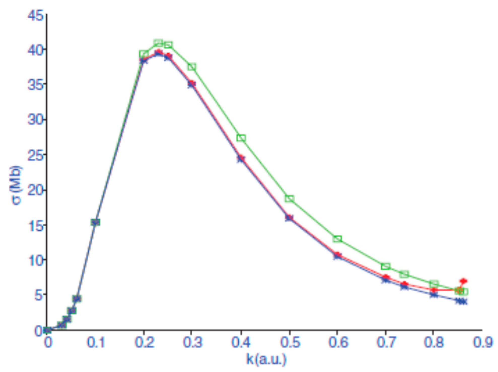
where γ = 0.2355883 and ρ = 2.646 ± 0.0004, γ is the square root of the binding energy of the electron and ρ is the effective range. The cross sections obtained using the effective-range theory are higher than those obtained in [27]. However, at low energies they are close to each other. Photodetachment cross sections for $H^{-}$are shown in Figure 1 from Ref. [27].

A similar calculation, including short-range and long-range correlations, has been carried out for the photoionization of He [27]. The results, given in

Table 8. Photoionization cross sections (Mb) of He [27] obtained with correlations.

k	${\mathit{N}}_{\mathit{\omega }}$ = 120	165	220	Ref. [30]	Ref. [31]
0.1	7.3319	7.3305	7.3300	7.295	7.44
0.2	7.1563	7.1549	7.1544	7.115	7.13
0.3	6.8733	6.8720	6.8716	6.838	6.83
0.4	6.4965	6.4953	6.4951	6.474	6.46
0.5	6.0471	6.0461	6.0461	6.006	6.02
0.6	5.5929	5.5924	5.5925	5.535	5.55
0.7	5.0121	5.0118	5.0120	4.985	5.04
0.8	4.4738	4.4738	4.4740	4.482	4.51
0.9	3.9647	3.9648	3.9649
1.0	3.4652	3.4654	3.4654	3.476	3.48
1.1	3.0205	3.0206	3.0206	3.023	3.00
1.3	2.2560	2.2561	2.2561	2.271	2.19
1.4	1.9820	1.9821	1.9821	1.943	1.89
1.5	1.6816	1.6817	1.6817
1.6	1.6324	1.6329	1.6329

, agree well with those obtained using the R-matrix approach [30] and the experimental results of Samson et al. [31]. Photoionization cross sections for Li ion have also been calculated and they are also given in [27].

We notice that in the limit $k\to 0$, the photodetachment cross section for H⁻ goes to zero because the plane wave is normalized as sin(kr)/kr which is equal to 1 for $r\to 0$, while the photoionization cross section of He goes to a finite value because of the final state Coulomb wave, which is proportional to $\frac{1}{\sqrt{k}}$ for $r\to 0$.

6. Recombination Rates

Knowing the photoabsorption cross sections, we can calculate radiative attachment rate coefficients which are important in the solar and astrophysical problems.

$$\begin{gathered} e+H\to H^{-}+hv \\ e+H{e}^{+}\to He+hv \end{gathered}$$

(64)

The attachment cross section σ_a is given by:

$$o_a={(\frac{hv}{c})}^2\frac{1}{2mE}\frac{g(f)}{g(i)}\sigma .$$

(65)

This relation follows from the principle of the detailed balance. The weight factors in the initial and final states are g(i) and g(f), E = k² is the energy of the electron, and $k_B$ is the Boltzmann constant in Equation (66), which gives the rate coefficient:

$${\alpha }_R(T)=\frac{(2S+1)10.2509x{10}^{10}}{{(T)}^{1.5}}\underset{0}{\overset{\infty }{\int }}dE{(E+I)}^2\sigma e^{-E/k_{B}T}.$$

(66)

In

Table 9. Recombination coefficients (cm³/s) for singlet states of H⁻, He, and Li⁺ [27].

T	αR(T) × 1015, H−	αR(T) × 1013, He	αR(T) × 1013, Li+
1000	0.99	2.50	0.12
2000	1.28	2.39	1.04
5000	2.40	1.87	2.62
7000	2.82	1.66	2.92
10,000	3.20	1.45	3.03
12,000	3.37	1.35	3.02
15,000	3.56	1.23	2.95
17,000	3.65	1.17	2.89
20,000	3.75	1.10	2.79
22,000	3.79	1.05	2.73
250,000	3.83	0.99	2.63
30,000	3.83	0.92	2.49
35,000	3.77	0.87	2.36
40,000	3.67	0.82	2.25

, the rate coefficients for the singlet states of H⁻, He, and Li⁺ are given at various temperatures [27]. We see that the rate coefficients for H⁻ and Li⁺ ions increase with temperature, attain a maximum value and then decrease, while in He atoms they decrease monotonically with the increase of the temperature.

Photoabsorption cross sections for excited states of the above systems and the recombination rate coefficients associated with these states have also been calculated [27]. In

Table 10. Rate coefficients (cm³/s) for (1s2s) ³S and (1s2s) 1S singlet excited states of He atom and Li⁺ ion [27].

T	He		Li+
	αR(T) × 1014, 3S	αR(T) × 1015, 1S	αR(T) × 1014, 3S	αR(T) × 1014, 1S
1000	2.13	8.27	4.68	2.99
2000	2.08	7.97	4.47	2.87
5000	1.73	7.30	3.48	2.27
7000	1.56	5.71	3.09	2.03
10,000	1.40	5.05	2.68	1.78
12,000	1.32	4.73	2.49	1.66
15,000	1.23	4.35	2.26	1.52
17,000	1.18	4.15	2.14	1.45
20,000	1.12	3.90	1.98	1.36
22,000	1.09	3.75	1.90	1.31
25,000	1.04	3.57	1.79	1.24
30,000	0.98	3.31	1.64	1.15
35,000	0.93	3.10	1.52	1.08
40,000	0.89	2.93	1.43	1.02

, rate coefficients for the excited states of He atoms and Li⁺ ions are given. As is well known, there are no excited states of H⁻, therefore no results are given for this ion. We see that the singlet and triplet states the rate coefficients differ quite a bit.

7. Excitation of the 2S State

Cross section for excitation of the 2S state of atomic hydrogen at low incident electron energies has been carried out using different methods. We mention a few: Burke et al. [32] used close-coupling approximation retaining 1s, 2s, and 2p eigenstates. Callaway et al. [33] carried out calculations in the range 12 to 54 eV using 11-state expansion including seven pseudostates. A similar calculation in the above energy range has been carried by Callaway et al. [34] using six-state close-coupling expansion including an optical potential. The results of these calculations are essentially based on the close-coupling approximation. Scott el al. [35] used the standard R-matrix close-coupling method using nine-state basis, consisting of three eigenstates and six pseudostates. Poet [36] carried out calculations by assuming spherically symmetric wave functions. Lloyd and McDowell [37] used the method of polarized orbitals for the first three partial waves and Bessel functions for the higher partial waves. All these results are different from each other. Even though the hydrogen atom is the simplest system, it seems it is not easy to get exact cross sections for excitation. Excitation cross sections have been calculated using the variational method of polarized orbitals [13]. The excitation cross section [38] from state ‘i’ to state ‘f’ is given by:

$$\sigma =\frac{k_f}{k_i}{\displaystyle \int |T_{fi}{|}^2}d\Delta .$$

(67)

where k_i and k_f are the initial and final momenta and T_fi is a matrix element given by:

$$T_{fi}=-(1/4\pi )\langle {\psi }_f\left|V\right|{\mathsf{\Psi }}_i\rangle .$$

(68)

The interaction potential is:

$$V=-\frac{2Z}{r_1}+\frac{2}{r_{12}}$$

(69)

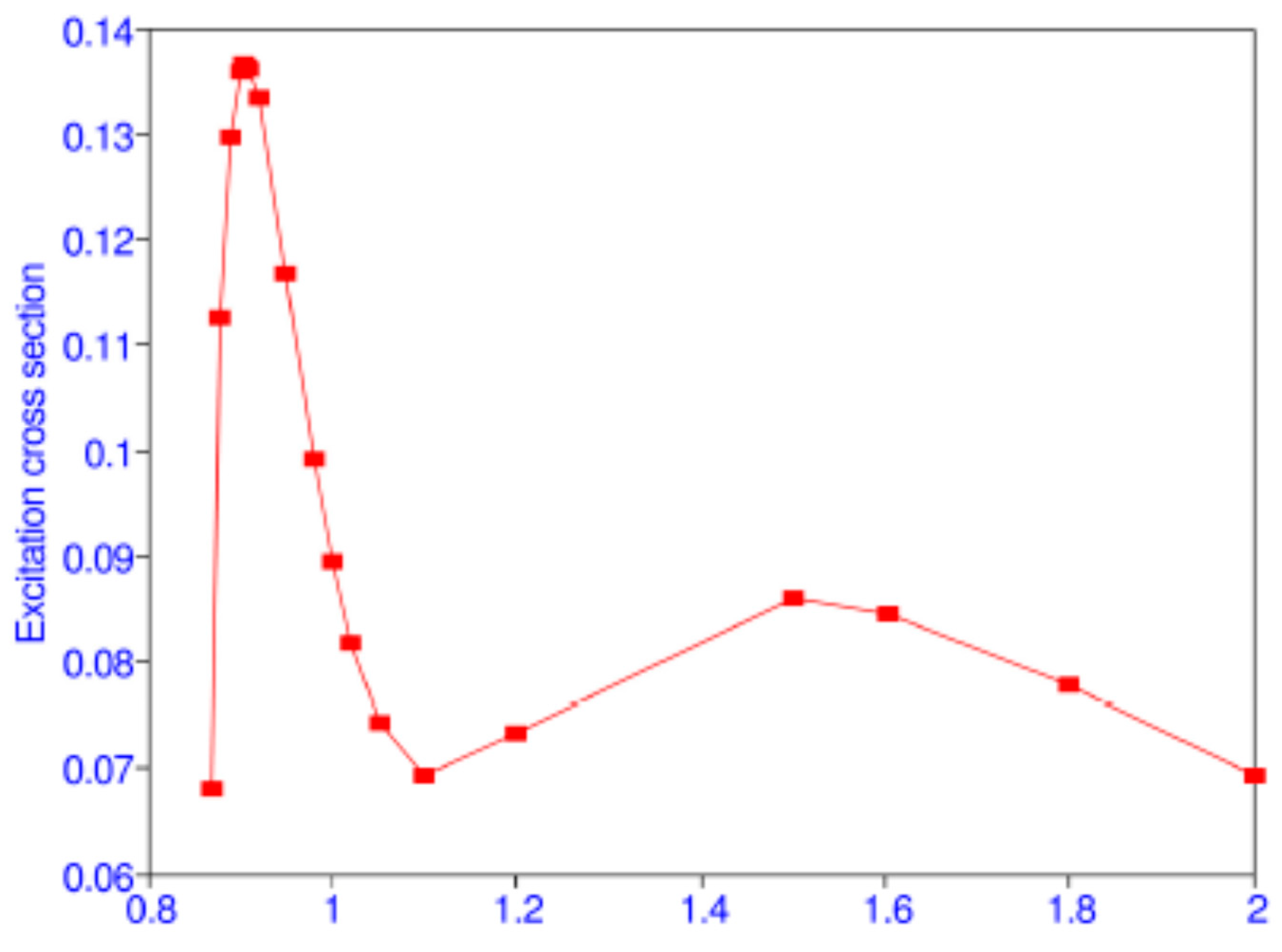
The initial state wave function ${\mathsf{\Psi }}_i$, in principle, is an exact solution of the Schrödinger equation [38]. Using this method, excitation cross sections have been calculated in the energy range 10.30 to 54.5 eV by using nine partial waves to get convergence, which is good up to the fifth and sixth decimal places for low energies, while at high energies it is good up to the third decimal place [38]. Some of the results of the various calculations are given in

Table 11. Excitation cross sections ($\pi a_0^2$) obtained in using variational polarized orbital method [40] and comparison with the results of other calculations.

K	Hybrid Theory [38]	Lloyd and McDowell [37]	Burke et al. [32]	Callaway [33]
0.87	6.8208(-2)
0.90	1.3589(-1)	0.1789	0.09918
0.904	1.3667(-1)
0.905	1.3673(-1)
0.906	1.3662(-1)
0.907	1.3660(-1)
0.98	9.9106(-2)			0.161
1.00	8.9474(-2)	0.1443	0.1783	0.154
1.02	8.1852(-2)			0.150
1.05	8.4057(-2)			0.142
1.10	6.9444(-2)		0.1654	0.135
1.20	7.3317(-2)		0.1349	0.111
1.50	8.5797(-2)		0.0891	0.087
1.60	8.4611(-2)			0.081
1.80	7.1804(-2)			0.074
2.00	6.9460(-2)	0.1198	0.06355	0.066

. The maximum of the cross section 0.137 $\pi a_0^2$ at 11.4 eV which is close to the experimental result 0.163 ± 0.2 $\pi a_0^2$ at 11.6 ± 0.2 eV of Kauppila et al. [39]. There is a minimum of the cross section at 16.46 eV and another maximum at 34.82 eV, as shown in Figure 2 from Ref. [38]. Differential and spin cross sections have also been calculated [38].

8. Lyman-Alpha Radiation

When the transition (2p- > 1s) takes place, we get electric dipole Lyman-alpha radiation which has a wavelength of 1216 A⁰ in H atoms and 304 A⁰ in He atoms. This radiation has been seen from the sun and from various astrophysical sources, and also from the Milky Way galaxy [41]. In most calculations, the 2p state is excited by electron impact. However, photoexciation is also possible: instead of leaving the target in the 1s state, it is left in the 2p state. The outgoing electron can then be in the final state l_f = 0 or 2. In the dipole approximation, the cross section is:

$$\begin{array}{l}\sigma =\frac{4\pi \alpha k\omega }{3(2l_i+1)}(|M_0{|}^2+|M_2{|}^2)\end{array}.$$

(70)

The matrix element M is defined as:

$$M={(2l_f+1)}^{0.5}|\langle {\mathsf{\Psi }}_f|z_1+z_2|{\mathsf{\Phi }}_i\rangle |.$$

(71)

In

Table 12. Photoabsorption cross sections (Mb) of the H anion, He, Li⁺, Be²⁺, and C⁴⁺. The final state is the ²P state [40].

K	H−	He	Li+	Be2+	C4+
0.1	1.2511	3.4706(-2)
0.2	1.6983	2.2972(-2)	3.8740(-3)	6.9296(-3)	1.8170(-4)
0.3	1.6578	3.0459(-2)	3.8183(-3)	6.7374(-3)	1.8144(-4)
0.4	1.1709	2.7627(-2)	3.7482(-3)	6.4820(-3)	1.8104(-4)
0.5	6.4369(-1)	2.4948(-2)	3.6694(-3)	6.1657(-3)	1.8048(-4)
0.6	4.4867(-1)	2.2717(-2)	3.5894(-3)	5.8193(-3)	1.7987(-4)
0.7	4.1448(-1)	2.1120(-2)	3.5102(-3)	5.4450(-3)	1.7916(-4)
0.8	3.5327(-1)	2.0058(-2)	3.4337(-3)	5.0471(-3)	1.7836(-4)
0.9	2.6847(-1)	1.9375(-2)	3.3712(-3)	4.6498(-3)	1.7505(-4)
1.0	1.508(-1)	1.8811(-2)	3.3083(-3)	4.2507(-3)	1.7641(-4)
1.1		1.8219(-2)	3.2481(-3)	3.8543(-3)	1.7552(-4)
1.2		1.7409(-2)	3.1894(-3)	3.4825(-3)	1.7437(-4)
1.3		1.6392(-2)	3.1220(-3)	3.1270(-3)	1.7322(-4)
1.4		1.5181(-2)	3.0533(-3)	2.8077(-3)	1.7198(-4)
1.5		1.3866(-2)	2.9777(-3)	2.4963(-3)	1.7072(-4)
1.6		1.2498(-2)	2.8919(-3)	2.2171(-3)	1.6963(-4)
1.7		1.1158(-2)	2.7898(-3)	1.9516(-3)	1.6819(-4)
1.8		9.8391(-3)	2.6849(-3)	1.7123(-3)	1.6678(-4)
1.9		8.6095(-3)	2.5735(-3)	1.4960(-3)	1.6521(-4)
2.0		7.4791(-3)	2.4546(-3)	1.3015(-3)	1.6371(-4)

, we give photoabsorption cross sections [40] for two-electron systems for various values of the outgoing electron leaving the photoionized target in 2p ²P state. The calculation in this problem has been carried out using only the exchange approximation for the final continuum states. No short-range and long-range correlations have been included in this calculation. The purpose was to show that the cross sections are significant and this process should be considered along with excitation by electron impact. Photoabsorption cross sections when the final state is 2s ²S instead of 2p ²P are also given in [40], along with the recombination rate coefficients.

9. Positron-Hydrogen Scattering

It should be noted that for positron-hydrogen scattering ${\mathsf{\Phi }}^{pol}$ has a positive sign instead of the negative sign as in the case of electron-hydrogen scattering:

$${\mathsf{\Phi }}^{pol}({\overrightarrow{r}}_1,{\overrightarrow{r}}_2)={\varphi }_0({\overrightarrow{r}}_2)+\frac{{\chi }_{ST}(r_1)}{r_1^2}\frac{u_{1s\to p}(r_2)}{r_2}\frac{\cos ({\theta }_{12})}{\sqrt{\pi Z}}.$$

(72)

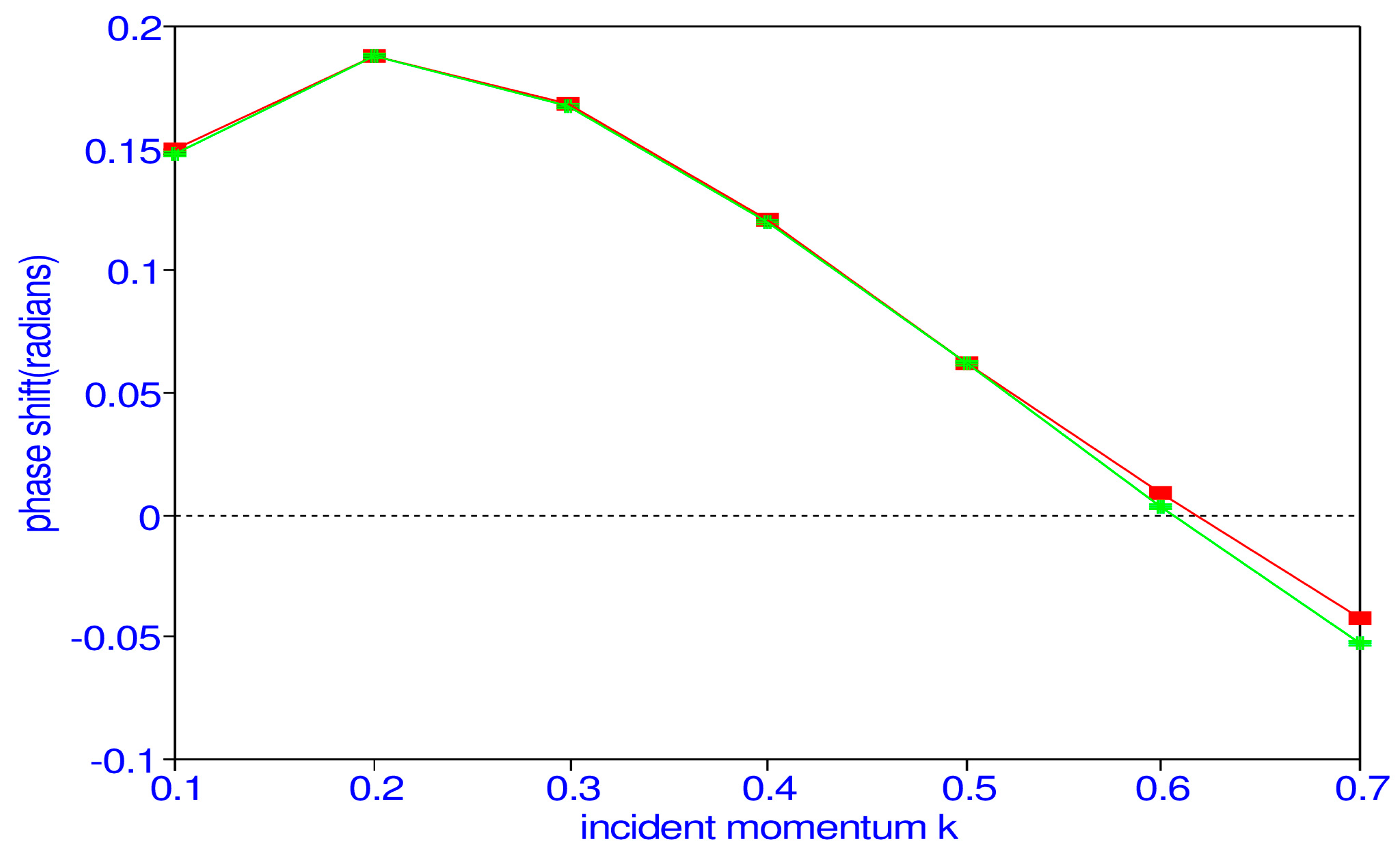
In

Table 13. Comparison of phase shifts (radians) for e⁺-H scattering for various k obtained in [42] with those obtained in [43].

k	Hybrid Theory [42]	P, Q Projections [43]	${\mathit{Z}}_{\mathit{e}\mathit{f}\mathit{f}}$
0.1	0.14918	0.1483	8.092
0.2	0.18803	0.1877	5.357
0.3	0.16831	0.1677	4.264
0.4	0.12083	0.1201	3.370
0.5	0.06278	0.0624	2.424
0.6	0.00903	0.0039	2.249
0.7	−0.04253	−0.0512	2.069

, we compare phase shift for S-wave scattering obtained in [42] using 35-term correlation functions with those obtained using 84-term correlation functions where projection operators were used [43]. With shorter expansions, improved results have been obtained, as also indicated in Figure 3 from Ref. [42].

The scattering length is −2.10258. Using the correction given in Equation (54), we find the scattering length is −2.104004 which agrees with −21036 ± 0.0004 obtained by Houston and Drachman [44], and with −2.103 ± 0.001 obtained by Humberston and Wallace [45].

10. Z_eff

There is a possibility of positronium annihilation for which the cross section is given by:

$${\sigma }_a(\pi a_0^2)=Z_{eff}{\alpha }^3/k.$$

(73)

Annihilation takes place with the emission of two gamma rays [46]. For hydrogen:

$$Z_{eff}={\displaystyle \iint d{\overrightarrow{r}}_{1}d{\overrightarrow{r}}_2|{\mathsf{\Psi }}_L({\overrightarrow{r}}_1,{\overrightarrow{r}}_2){|}^2\delta ({\overrightarrow{r}}_1,{\overrightarrow{r}}_2).}$$

(74)

The normalization of the scattering function for $r_1\to \infty$ is given by:

$$u_L(r_1)={[4\pi (2L+1)]}^{0.5}\sin (k{r}_1-\frac{L\pi }{2}+\eta )/k.$$

(75)

11. Positronium Formation

Positronium formation takes place when the incident positron captures an electron of the hydrogen target:

$$e^{-}+H(1s)\to Ps+P.$$

(76)

Z_eff and positronium formation have been calculated [42] using hybrid theory. The results for Z_eff are given in Table 13 and positronium formation cross sections are given in [42]. A similar calculations have been carried out for P-wave scattering. Z_eff and positronium formation cross sections have also been calculated [47].

12. Conclusions

In summary, we have used an approximation for scattering calculations in which the long-range and short-range correlations have been included at the same time variationally. The phase shifts for electron and positron scattering have a lower bound to the exact phase shifts. We have used these continuum functions to calculate resonance parameters, photoabsorption, and excitation cross sections, Z_eff and positronium formation cross sections. The results are in agreement with those obtained in other calculations.

References

- Morse, P.M.; Allis, W.P. The effect of Exchange on the Scattering of Slow Electrons from Atoms. Phys. Rev. 1933, 44, 269. [Google Scholar] [CrossRef]
- Kohn, W. Variational Methods in Nuclear Collision Problems. Phys. Rev. 1948, 74, 1763. [Google Scholar] [CrossRef]
- Schwartz, C. Electron Scattering from Hydrogen. Phys. Rev. 1961, 124, 1468. [Google Scholar] [CrossRef]
- Burke, P.G.; Smith, K. The Low-Energy Scattering of Electrons and Positrons by Hydrogen Atoms. Rev. Mod. Phys. 1962, 34, 458. [Google Scholar] [CrossRef]
- Burke, P.G.; Robb, W.D. The R-matrix Theory of Atomic Processes. Adv. At. Mol. Phys. 1976, 11, 143. [Google Scholar]
- Temkin, A.; Lamkin, J.C. Application of the Method of Polarized Orbitals to the scattering of Electrons from Hydrogen. Phys. Rev. 1961, 121, 788. [Google Scholar] [CrossRef]
- Bhatia, A.K.; Temkin, A. Complex-correlation Kohn T-matrix method of calculating total and elastic cross sections: Electron-hydrogen elastic scattering. Phys. Rev. A 2001, 64, 032709. [Google Scholar] [CrossRef]
- Wigner, E.P. On the Behavior of Cross Sections Near Threshold. Phys. Rev. 1948, 73, 1002. [Google Scholar] [CrossRef]
- Temkin, A. A note on the Scattering of Electrons from Atomic Hydrogen. Phys. Rev. 1959, 116, 358. [Google Scholar] [CrossRef]
- Sloan, I.H. The method of polarized orbitals for the elastic scattering of slow electrons by ionized helium and atomic hydrogen. Proc. R. Soc. Lond. A 1964, 281, 151–163. [Google Scholar] [CrossRef]
- Feshbach, H. A unified theory of nuclear reactions. II. Ann. Phys. 1962, 19, 287–313. [Google Scholar] [CrossRef]
- Bhatia, A.K.; Temkin, A. Symmetric Euler-Angle Decomposition of the Two-Electron Fixe-Nucleus Problem. Rev. Mod. Phys. 1964, 36, 1050. [Google Scholar] [CrossRef]
- Bhatia, A.K. Hybrid theory of electron-hydrogen elastic scattering. Phys. Rev. A 2007, 75, 032713. [Google Scholar] [CrossRef]
- Shertzer, J.; Temkin, A. Direct calculation of the scattering amplitude without partial-wave analysis III. Inclusion of correlation effects. Phys. Rev. A 2006, 74, 052701. [Google Scholar] [CrossRef]
- Scholz, T.; Scott, P.; Burke, P.G. Electron-hydrogen-atom scattering at intermediate energies. J. Phys. B 1988, 21, L139. [Google Scholar] [CrossRef]
- Bhatia, A.K. Applications of the hybrid theory in the scattering of electrons from He+ and Li2+ and resonances in these systems. Phys. Rev. A 2008, 77, 052707. [Google Scholar] [CrossRef]
- Gien, T.T. Accurate calculation of phase shifts for electron-He+ collisions. J. Phys. B 2002, 35, 4475. [Google Scholar] [CrossRef]
- Gien, T.T. Accurate calculation of phase shifts for electron collisions with positive ions. J. Phys. B 2003, 36, 2291. [Google Scholar] [CrossRef]
- Bhatia, A.K. Hybrid theory of P-wave electron-hydrogen elastic scattering. Phys. Rev. A 2012, 85, 052708. [Google Scholar] [CrossRef]
- Bhatia, A.K. Application of P-wave hybrid theory in the scattering of electrons from He+ and resonances in He and H−. Phys. Rev. A 2012, 86, 032709. [Google Scholar] [CrossRef]
- Botero, J.; Shertzer, J. Direct numerical solution of the Schrödinger equation for the quantum scattering problems. Phys. Rev. A 1992, 46, R1155. [Google Scholar] [CrossRef] [PubMed]
- Bhatia, A.K. D-wave electron-H, He+, and Li2+ elastic scattering and photoabsorption in P states of two-electron system. Phys. Rev. A 2014, 89, 062720. [Google Scholar] [CrossRef]
- Temkin, A. Polarization and Triplet Electron-Hydrogen Scattering Length. Phys. Rev. Lett. 1961, 6, 354. [Google Scholar] [CrossRef]
- Bhatia, A.K.; Temkin, A. Calculation of autoionization of He and H− using the projection-operator formalism. Phys. Rev. A 1975, 11, 2018. [Google Scholar] [CrossRef]
- O’Malley, T.F.; Rosenberg, L.; Spruch, L. Low-Energy Scattering of a charged Particle by a Neutral Polarizable System. Phys. Rev. 1962, 125, 1300. [Google Scholar] [CrossRef]
- Wildt, R. Electron Affinity in Astrophysics. Astrophys. J. 1939, 89, 295–301. [Google Scholar] [CrossRef]
- Bhatia, A.K. Hybrid theory of P-wave electron-Li2+ elastic scattering and photoabsorption in two-electron systems. Phys. Rev. A 2013, 87, 042705. [Google Scholar] [CrossRef]
- Bell, K.L.; Kingston, A.E. The bound-free absorption coefficient of the negative hydrogen ion. Proc. Phys. Soc. Lond. 1967, 90, 895. [Google Scholar] [CrossRef]
- Ohmura, T.; Ohmura, H. Electron-Hydrogen Scattering at low energies. Phys. Rev. 1960, 118, 154. [Google Scholar] [CrossRef]
- Nahar, S.N. New Quests in Stellar Astrophysics. II. The Ultraviolet Properties of Evolved Stellar Populations; Chavez, M., Bertone, E., Rosa-Gonzalez, D., Rodriguez-Merino, L.H., Eds.; Springer: New York, NY, USA, 2009; p. 245. [Google Scholar]
- Samson, J.A.R.; He, Z.X.; Yin, L.; Haddad, G.H. Precision measurements of the absolute photoionization cross sections of He. J. Phys. B 1994, 27, 887. [Google Scholar] [CrossRef]
- Burke, P.G.; Schey, H.M.; Smith, K. Collisions of Slow Electrons and Positrons with Atomic Hydrogen. Phys. Rev. 1963, 129, 1258. [Google Scholar] [CrossRef]
- Callaway, J. Scattering of electrons by atomic hydrogen at intermediate energies: Elastic Scattering and n = 2 excitation from 12 to 54 eV. Phys. Rev. A 1985, 32, 775. [Google Scholar] [CrossRef]
- Callaway, J.; Unnikrishnan, K.; Oza, D.H. Optical potential of electron-hydrogen scattering at intermediate energies. Phys. Rev. A 1987, 36, 2576. [Google Scholar] [CrossRef]
- Scott, M.P.; Scholz, T.T.; Walters, H.R.; Burke, P.G. Electron scattering by atomic hydrogen at intermediate energies: Integrated elastic, is-2s and 1s-2p cross sections. J. Phys. B 1989, 22, 3055. [Google Scholar] [CrossRef]
- Poet, R. The exact solution for a simplified model of electrons scattering by hydrogen atoms. J. Phys. B 1978, 11, 3081. [Google Scholar] [CrossRef]
- Lloyd, M.D.; McDowell, M.R.C. An application of the polarized approximation to electron-impact excitation of atomic hydrogen. J. Phys. B 1969, 2, 1313. [Google Scholar] [CrossRef]
- Bhatia, A.K. Excitation of the 2S State of Atomic Hydrogen by Electron Impact. Atoms 2018, 6, 7. [Google Scholar] [CrossRef]
- Kauppila, W.E.; Ott, W.R.; Fite, W.L. Excitation of Atomic Hydrogen to the Metastable 22S1/2 State by Electron-Impact. Phys. Rev. A 1970, 1, 1099. [Google Scholar] [CrossRef]
- Bhatia, A.K.; Drachman, R.J. Photoejection with excitation in H− and other systems. Phys. Rev. A 2015, 91, 012702. [Google Scholar] [CrossRef]
- Lallement, R.; Que’merais, E.; Bertaux, J.-L.; Sandel, B.R.; Izmodenov, V. Voyager Measurements of Hydrogen Lyman-α Diffuse Emission from the Milky Way. Science 2011, 334, 1665–1669. [Google Scholar] [CrossRef] [PubMed]
- Bhatia, A.K. Positron-Hydrogen Scattering, Annihilation, Positronium Formation. Atoms 2016, 4, 27. [Google Scholar] [CrossRef]
- Bhatia, A.K.; Temkin, A.; Drachman, R.J.; Eiserike, H. Generalized Hylleraas Calculation of Positron-Hydrogen Scattering. Phys. Rev. A 1971, 3, 1328. [Google Scholar] [CrossRef]
- Houston, S.K.; Drachman, R.J. Positron-Atom by Kohn and Harris Methods. Phys. Rev. A 1971, 3, 1335. [Google Scholar] [CrossRef]
- Humberston, J.W.; Wallace, J.B.G. The elastic scattering of positrons by atomic hydrogen. J. Phys. B 1972, 5, 1138. [Google Scholar] [CrossRef]
- Ferrall, R.A. Theory of Positron Annihilation in Solids. Rev. Mod. Phys. 1956, 28, 308. [Google Scholar] [CrossRef]
- Bhatia, A.K. P-wave Positron-Hydrogen Scattering, Annihilation, and Positronium Formation. Atoms 2017, 5, 17. [Google Scholar] [CrossRef]
Figure 1.
Photodetachment of detachment of a hydrogen ion. The lowest curve is obtained only when the long-range correlations are included; the middle curve is obtained when the short-range and long-range correlations are included. The top [27] curve is obtained when the effective range theory and the loosely bound structure of hydrogen ion used [29].
Figure 2.
(Color online) Total 1S–2S excitation cross section () vs. the incident momentum k(Ryd).
Figure 3.
(Color online) The upper curve represents the present results, while the lower curve represents obtained by Bhatia et al. [43].