Ant Robotic Swarm for Visualizing Invisible Hazardous Substances


1
Centre for Research in Distributed Technologies, University of Bedfordshire, Park Square, Luton, LU1 3JU, UK
2
School of Computer Science and Electronic Engineering, University of Essex, Colchester CO4 3SQ, UK
*
Author to whom correspondence should be addressed.
Robotics 2013, 2(1), 1-18; https://doi.org/10.3390/robotics2010001
Submission received: 8 November 2012
/
Revised: 21 December 2012
/
Accepted: 4 January 2013
/
Published: 7 January 2013
(This article belongs to the Special Issue Human Centred Robotics)
Abstract
:Inspired by the simplicity of how nature solves its problems, this paper presents a novel approach that would enable a swarm of ant robotic agents (robots with limited sensing, communication, computational and memory resources) form a visual representation of distributed hazardous substances within an environment dominated by diffusion processes using a decentralized approach. Such a visual representation could be very useful in enabling a quicker evacuation of a city’s population affected by such hazardous substances. This is especially true if the ratio of emergency workers to the population number is very small.
1. Introduction
Monitoring of hazardous substances in our environments is fast becoming a high priority for governments around the world due to global warming [1,2,3]. One of the projects that have been setup to tackle pollution is the European Union Shoal project, in which a shoal of robotic fishes would be deployed to find the source of pollution in sea ports and the culprit responsible charged accordingly. This work focuses on the spread of pollution by diffusion in the hydrodynamics section of the European Union Shoal project. Monitoring of hazardous substances in environments other than the sea is also a necessity. This is especially true if the hazardous substance is not visible to humans. Such substances could include nerve gas, Carbon dioxide, which can be fatal if in large quantities, Sarin gas or even nuclear radiation. Taking a scenario in which nerve gas as been released due to a terrorist attack in a city; the population of that city needs to be evacuated. However, as they cannot see the pollution, they do not know whether they are running towards it or away from it. The emergency services have been called in but are overwhelmed by the ratio of number of citizens to crew men. If however a swarm of flying micro robots were able to visualize the pollutant, it is possible for the population to keep away from affected areas and in the process evacuate themselves from dangerous areas.
This can be done by ensuring that the motion of each individual agent in the swarm of robots is controlled so that eventually, the distribution of the swarm converges in a way that areas containing a high amount of pollutants are more densely covered by swarm individuals than areas that have little or no pollutant. This approach leads to efficient use of mobile sensors especially when their numbers are limited.
Furthermore, the robots could be used as measurement stations to collect information about the pollutant and then a map of the pollution could be developed and built at a ground station. This information could then be used to predict the path and behaviour of the invisible pollutant. By observing the behaviour of the pollutant from the map, it is possible to say what type of pollutant it is. In order for the agents to provide such visual information, the agents need to be equipped with a coverage control algorithm that would enable them to perform optimal coverage.
There has been a lot of work done in the area of coverage using multiple agents, such as the use of Voronoi partitions [4,5,6,7,8]. The Voronoi partition method requires a polygon derived environment and a large computational time due to computation of the Voronoi partition in addition to the computation of the global cost function required to drive the mobile sensors to their required cost minimal positions. Nevertheless, Schwager et al. was able to use the Voronoi partition method and a Radial basis function machine learning technique on a group of robots to achieve a visual representation in [6,9]. Shucker et al. [10,11] used virtual springs to form the distribution of a pollutant by tracking points in it. Their work requires long distance communication and this might not be possible when considering hardware limitations on simple agents.
The use of deterministic annealing as in [12] also requires a large communication burden. Artificial Physics and Computation Fluid Dynamics (CFD) were used by Zarzhitsky et al. in [13] to control a group of robots to find the source of a pollutant in the environment. Artificial Physics was used to make the robots form a lattice while CFD was used to navigate up pressure fluxes in the environment towards the source. This approach works on the assumption that the pollutant would most likely to be in the area where there was a negative flux or sink.
Furthermore, work has also been carried out regarding coverage using ant robots. Ant robotics has been inspired by simple minded creatures like ants whereby individuals following simple rules are able to build complex structures and perform complex feats of engineering. Robots inspired by these creatures often have limited memory, computing, sensing and communication resources [14,15]. These properties make them very cheap and hence disposable in hazardous situations whereby they could be thrown away after being used for monitoring harmful substances. Additionally, most of the work in ant robotics tend to focus on simple algorithms to perform tasks such as lawn mowing, mine sweeping, vacuum cleaning, and so on, and make use of the advantage of multiple agents to introduce graceful degradation of the system [15].
In [14], terrain coverage by ant robots was investigated. In their work, they took inspiration from natural ants by using markings left by individual robots to communicate indirectly with other individual robots. Additionally, the markings were also used to determine the next action of the ant due to its ability to sense what is around it. Their ant robots did not need a map of the terrain, localization, path planning nor did they require memory. They were able to achieve terrain coverage by comparing a variety of algorithms such as Learning Real-time A Star (LRTA*), Node counting, Thrun’s Value-Update Rule and Wagner’s Value-Update Rule.
In the famous “cooperative cleaners” task in [16], a cleaning protocol algorithm called CLEAN was developed to clean up contaminated tiles in the environment. In [17], a dynamic cleaning algorithm called SWEEP was developed to clean up a dynamically spreading target such as fire. However, this work and that in [18] relies on the fact that critical points are not cleaned so that the task can be completed. Furthermore, in [18], a distributed search for evasive targets using ant robots was presented while in [19] analyses of how many pursuers and how they should move was conducted. Similarly, [18] analysed the amount of time it would take for a swarm of robots to clean both a static and expanding region of pollutants while in [15], the authors showed that even if robots having limited capabilities were moved, it is guaranteed that a swarm of them would still cover an area of interest. In most of the work above, algorithms were either developed or applied after understanding the nature of the problem.
This work uses mathematical models of the bacterium, flocking behaviour as seen in starlings and a velocity function to solve the problem of providing a visual representation of an invisible pollutant.
The bacterium behaviour was used to explore the environment, find pollutants and subsequently navigate up the gradient of the pollutant; the flocking behaviour was used to keep agents from colliding from each other and for collective foraging; while the velocity function was used to simulate a dwelling behaviour in which agents tend to dwell in an area that has a rich source of food compared to other areas that lack food.
This work is divided into two parts. The first part uses a swarm of robots to provide a visual representation of a static pollutant and follows in the path of ant robots. Using the criteria in [15], the robots have a finite bounded memory k = 4 and communication radius of r = 50 in a grid of 2000 by 2000. Additionally, the agents can only sense the pollutant in their immediate locality (x, y) but cannot sense what is beyond this at for example (x ± ∆x, y ± ∆y). Using this information, each individual agent moves according to a set of equations that model the bacterium’s behaviour when searching for food. The bacterium only needs current local information related to the area in which it presently is; in addition to a history of past local information k = 4 in order to determine its next move.
This is unlike previous work in ant robotics where most of the work relied on assuming that the ant knows about the conditions in tiles surrounding it. The conditions in those tiles then determine its next action.
Also, in this present work, cleaning is not our major objective. The effect of cleaning on the proposed algorithm in this work would be studied in future work. Nevertheless, this is the first time that ant robots have been used in the task of visualizing pollutant.
The second part investigates the possibility of enhancing the first part by using a Genetic Algorithm machine learning technique. In this case, the ant robots are equipped with knowledge of the pollutant profile to be mapped. We do this in accordance to [20] in which Arkin discussed how simple reactive models of robot control could be made more effective through the introduction of knowledge about the environment. This was done in this work by updating the parameters of the proposed ant coverage controller through the use of a modified computationally efficient Gaussian model based Genetic Algorithm. The Genetic Algorithm was used to estimate the distribution of the pollutant in the environment and the information used as a cost function to distribute the agents optimally in the environment. However, it could be argued that introducing this additional capability makes them less of ant robots due to the computational expensive nature of Genetic Algorithms.
Furthermore, it should be noted that the method presented in this work does not require the geometry of the environment to be known a priori as in the Voronoi partition method [21]. Also, the approach uses computationally efficient ant algorithms to achieve the same level of coverage as was investigated in [22].
The rest of this paper is arranged as follows. In Section 2, the technical approach is described, including the problem description and coverage controller. Section 3 discusses, briefly, about how a Genetic Algorithm was used to estimate the profile of a pollutant in the environment while Section 4 discusses about simulation results. Finally, a brief conclusion and future work are presented in Section 5.
2. Technical Approach
The problem of distributing sensors into an environment under investigation can be seen as a coverage problem in which a pollution profile F(S(x)) presented in an area S(x) is to be covered by n number of robotic agents so that the distribution of the robotic agents AT (x) is close to that of the pollution profile F(S(x)) where x is the set of coordinates (x, y) in S(x). The robotic agents used in this work are assumed to have omnidirectional kinematics.
However, the proposed coverage controller can also be used on other types of robotic platforms with different dynamics by adding a low level controller to convert the control outputs into ones that suitable for the platform being used.
As mentioned previously, the coverage controller is made up of a bacteria controller that gives the agents the ability to navigate up a pollution gradient or a pressure flux gradient if required. This controller gives a source directional force to the flock of agents. A flocking controller is used to make the agents move as a group towards the source of the pollutant and to pull each other out of local minimum situations if they occur. Additionally, the flocking controller enables the flock of agents to localise at the source faster than if they were moving individually. The velocity controller is used to tune the distribution of the agents in the environment as will be discussed in Section 2.3. Each controller will now be discussed separately.
2.1. Bacteria Controller
There have been many investigations into the development of pollution source seeking controllers. For example Baronov and Baillieul [23], used a radial function as a potential function to develop an ascending controller. Their algorithm is not fully dependent on gradient but the function to be mapped or transverse must be known a priori for tuning the controller. Mayhew et al. [24] used a hybrid controller that combines a line minimization-based algorithm and a vehicle path planning algorithm to find the extremum of a function. Their approach does not need GPS point measurements and does not need any knowledge of the function to be mapped a priori. Dhariwal [25] used the Keller and Segel bacteria model as a basis for developing their controller whilst Marques et al. [26] investigated the use of rule based approach to using bacteria chemotaxis behaviour on a robot. In their experiments, they also investigated the use of the silkworm moth algorithm and a direct gradient following method. Lilienthal et al. [27] used a Braitenberg vehicle approach to find an ethanol source in their own experiments.
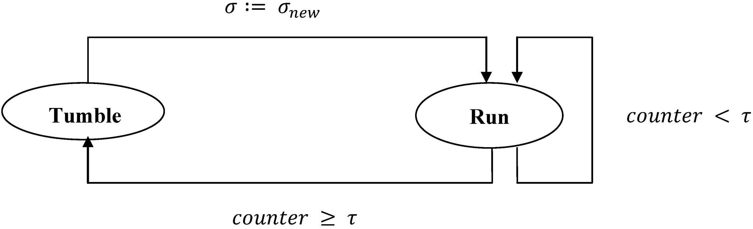
However this work uses a controller based on the Berg and Brown model in [28]. Models such as the one in [29], and other modern complex models, were not considered because a random biased walk model is sufficient for environmental exploration and source declaration in an environment. A bacterium motion is composed of a combination of tumble and run phases. The frequency of these phases depends on the measured concentration gradient in the surrounding environment. The run phase is generally a straight line while the tumble phase is a random change in direction with a mean of about 68 degrees in the E. Coli bacterium. If the bacterium is moving up a favourable gradient, it tumbles less thereby increasing the length of the run phase and vice versa if going down an unfavourable gradient. This behaviour was modelled by Berg and Brown by fitting the results of their experimental observations in [30] with a best fit equation in [28]. This model is shown below:
![Robotics 02 00001 i001]()
![Robotics 02 00001 i002]()
![Robotics 02 00001 i003]() where τ is the mean run time and τ0 is the mean run time in the absence of concentration gradients, α is a constant of the system based on the chemotaxis sensitivity factor of the bacteria, Pb is the fraction of the receptor bound at concentration C. In our work, C was the present reading taken by our Robotic agent. kD is the dissociation constant of the bacterial chemoreceptor.
where τ is the mean run time and τ0 is the mean run time in the absence of concentration gradients, α is a constant of the system based on the chemotaxis sensitivity factor of the bacteria, Pb is the fraction of the receptor bound at concentration C. In our work, C was the present reading taken by our Robotic agent. kD is the dissociation constant of the bacterial chemoreceptor. ![Robotics 02 00001 i019]() is the rate of change of Pb.
is the rate of change of Pb. ![Robotics 02 00001 i020]() is the weighted rate of change of Pb, while τm is the time constant of the bacterial system.
is the weighted rate of change of Pb, while τm is the time constant of the bacterial system.


 is the rate of change of Pb.
  is the weighted rate of change of Pb, while τm is the time constant of the bacterial system.
 The above equations determine the time between tumbles and hence the length of runs between tumbles. During the tumble phase, the robot agent can randomly choose a range of angles in the set σ ∈ {0…… 360} by randomly choosing angles. This made it possible for the robot agents to backtrack if there is a favourable gradient behind it. The ability of the implemented bacteria chemotaxis controller to work over long distances has been presented in [31,32] and works fine even in the presence of small disturbances.
The above discussion about the bacterium behaviour can be depicted graphically, as shown in Figure 1.
A counter that increments every time tick is implemented. Once the counter is greater than τ a tumble phase is initiated otherwise the bacterium stays in the run phase. Once a tumble phase is completed through the assigning of a new σ, the run phase is resumed. A velocity controller which will be discussed in Section 2.3 was embedded into the bacterium controller.
It could be argued that the bacterium behaviour is a gradient based algorithm and, as such, an ordinary gradient based algorithm could be used in place of it. However, the Equations (1) to (3) have more to them than meets the eye. These equations take noise in the bacterium sensors, dynamics or environment into consideration. Equation (2) is an exponentially weighted low pass filter that is capable of filtering out noise. As a result of the filter, the Berg and Brown derived bacterium controller is not easily affected by noise and hence would not be readily caught in local maximums when they are encountered [33]. This is further aided by the random nature of the algorithm as a result of the tumble phase of the controller.
Figure 1.
Showing the transitions between the two bacterium phases.
It could be argued as well that the random nature of the algorithm is not beneficial to bacteria. However, as was proven in [34], it is this very random nature that enables them to form a distribution corresponding to the profile of the pollutant in the environment. This is further supported by the works of Mach and Schweitzer, Hamann and Heinz [35,36] in which they discussed how a swarm of stochastic agents having a random component (bacterium tumble phase in this case) and a direct component (bacterium run phase in this case) can be represented by a Fokker Planck equation. The Fokker Planck equation would always converge to its stationary distribution that corresponds to the spatial function of interest.
It is the above properties that make the Berg and Brown derived bacterium controller different from an ordinary gradient ascent algorithm, and make it suited for use on noisy functions as used in the simulations in this work. In this work, the filter as represented by Equation (2) was implemented in discrete form using an ant limited memory resource length k = 4 to remember a history of past readings.
2.2. Flocking Controller
There has been a lot of work done on flocking controllers. The first flocking controller was developed by C.W. Reynolds in [37]. In order to achieve flocking, he defined that three rules need to followed. These rules were: Keep as close as possible to your neighbour (Aggregation), do not collide with your neighbour (Collision Avoidance), and move in a similar general heading as your neighbours.
Following this discovery, many researchers such as [38,39,40] have worked on these three basic rules in investigating various approaches of achieving flocking. Most of the approaches agree that Equation (4) should be satisfied in order to achieve flocking [38].
![Robotics 02 00001 i004]() where r is the distance between agents, GR
where r is the distance between agents, GR ![Robotics 02 00001 i021]() represents the repulsion function and GA
represents the repulsion function and GA ![Robotics 02 00001 i021]() is the attractive function. Following this, we use exponential functions, as in Equation (5), to achieve flocking. This results in the Morse potential as in Equation (5) [41].
is the attractive function. Following this, we use exponential functions, as in Equation (5), to achieve flocking. This results in the Morse potential as in Equation (5) [41].
![Robotics 02 00001 i005]()
![Robotics 02 00001 i006]() where i is the index of the agents. Gains of 1 for the repulsion term GR and 0.99 for the attractant term GA were used. It was discovered that it is possible to control how closely the agents get to each other whilst not colliding by reducing the GG gain. r in Equation (5) is the distance between the two closest agents. This value was obtained as follows: Each agent had a communication radius l = 50 and can only buffer up to N = 5 readings obtained from agents within this range. From these readings, the closest agent r is obtained and this value is used in Equation (5) to avoid collisions with other agents. Despite using a limited number N of neighbours, the agents were still able to avoid collisions whilst maintaining cohesion as a flock. Using a buffer of five readings was used only for flocking. This buffer is not necessary if proximity sensors are used instead, making sure that the ant like feature is maintained.
where i is the index of the agents. Gains of 1 for the repulsion term GR and 0.99 for the attractant term GA were used. It was discovered that it is possible to control how closely the agents get to each other whilst not colliding by reducing the GG gain. r in Equation (5) is the distance between the two closest agents. This value was obtained as follows: Each agent had a communication radius l = 50 and can only buffer up to N = 5 readings obtained from agents within this range. From these readings, the closest agent r is obtained and this value is used in Equation (5) to avoid collisions with other agents. Despite using a limited number N of neighbours, the agents were still able to avoid collisions whilst maintaining cohesion as a flock. Using a buffer of five readings was used only for flocking. This buffer is not necessary if proximity sensors are used instead, making sure that the ant like feature is maintained.

 represents the repulsion function and GA is the attractive function. Following this, we use exponential functions, as in Equation (5), to achieve flocking. This results in the Morse potential as in Equation (5) [41].


The final output from the flocking controller and bacteria controller is calculated as shown in Equation (6) where GF and GB are gains applied to both the flocking controller and bacteria controller output respectively.
2.3. Velocity Controller
The agent velocity updates are such that by controlling them, it is possible for the agents form a distribution of the pollutant in the environment and in works of [32,42] it was obtained by an adaptable velocity that was determined by Equation (7):
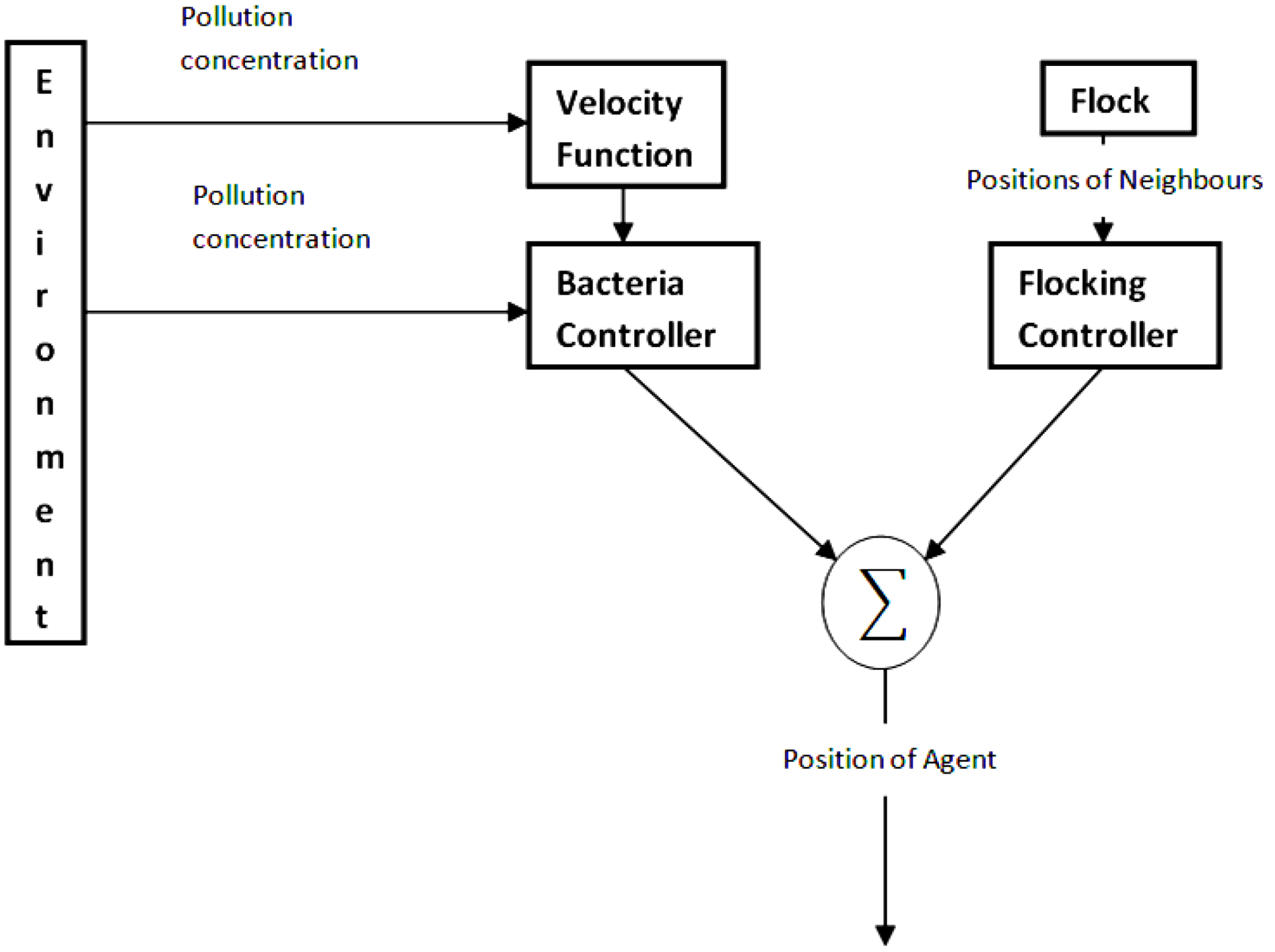
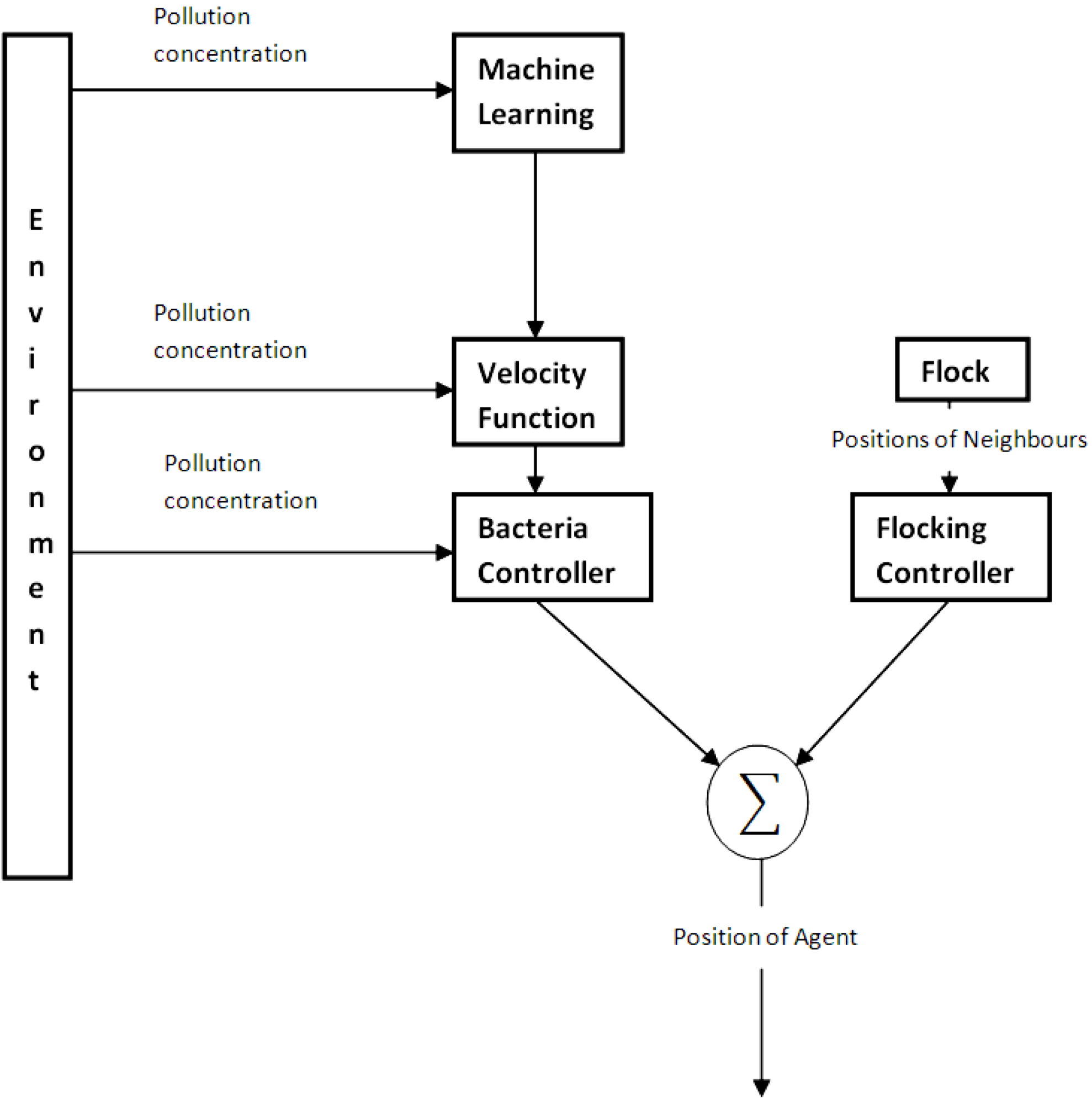
![Robotics 02 00001 i007]() where β is a dynamic velocity that depends on the present reading of the environmental quantity, βo is the standard velocity without any reading, vk is a constant for tuning the dynamic velocity and C is the pollutant reading obtained by the robot’s sensor. The separate controllers are combined by using the architecture shown in Figure 2.
where β is a dynamic velocity that depends on the present reading of the environmental quantity, βo is the standard velocity without any reading, vk is a constant for tuning the dynamic velocity and C is the pollutant reading obtained by the robot’s sensor. The separate controllers are combined by using the architecture shown in Figure 2.

The relationship between the bacterium controller and the velocity controller is shown in Equation (8), where distτ is the distance covered by the agent during a run phase and tτ is the time duration from the last tumble phase.
![Robotics 02 00001 i008]()

By using the velocity Equation (7), it was possible to enable agents achieve various visual distributions of pollution profiles as can be seen in Figure 2, Figure 3, Figure 4 and Figure 5. However, it was also discovered that the constant vk, can be used to control the spread of the agents in the pollution profile with high vk values resulting in agents behaving more like gas molecules, covering a smaller area and forming less detailed features of the pollution profile whilst lower vk values result in agents behaving more like liquid-like molecules, covering a higher area and showing more detailed features of the pollutant profile as can be seen in Figure 6 and Figure 7.
By using the velocity Equation (7), it was possible to enable agents achieve various visual distributions of pollution profiles as can be seen in Figure 2, Figure 3, Figure 4 Figure 5. However, it was also discovered that the constant vk, can be used to control the spread of the agents in the pollution profile with high vk values resulting in agents behaving more like gas molecules, covering a smaller area and forming less detailed features of the pollution profile whilst lower vk values result in agents behaving more like liquid-like molecules, covering a higher area and showing more detailed features of the pollutant profile as can be seen in Figure 6 and Figure 7.
Figure 2.
Architecture of coverage controller.

Figure 3.
Simulated Arena with Gaussian distributed agents (a); Gaussian shaped distribution of pollutant (b).
Figure 3.
Simulated Arena with Gaussian distributed agents (a); Gaussian shaped distribution of pollutant (b).
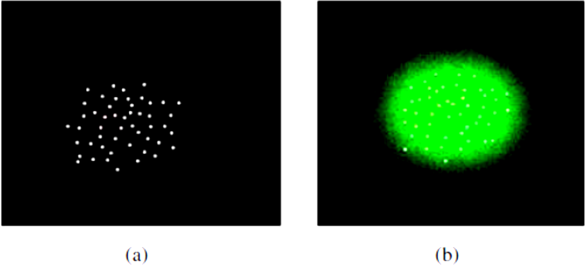
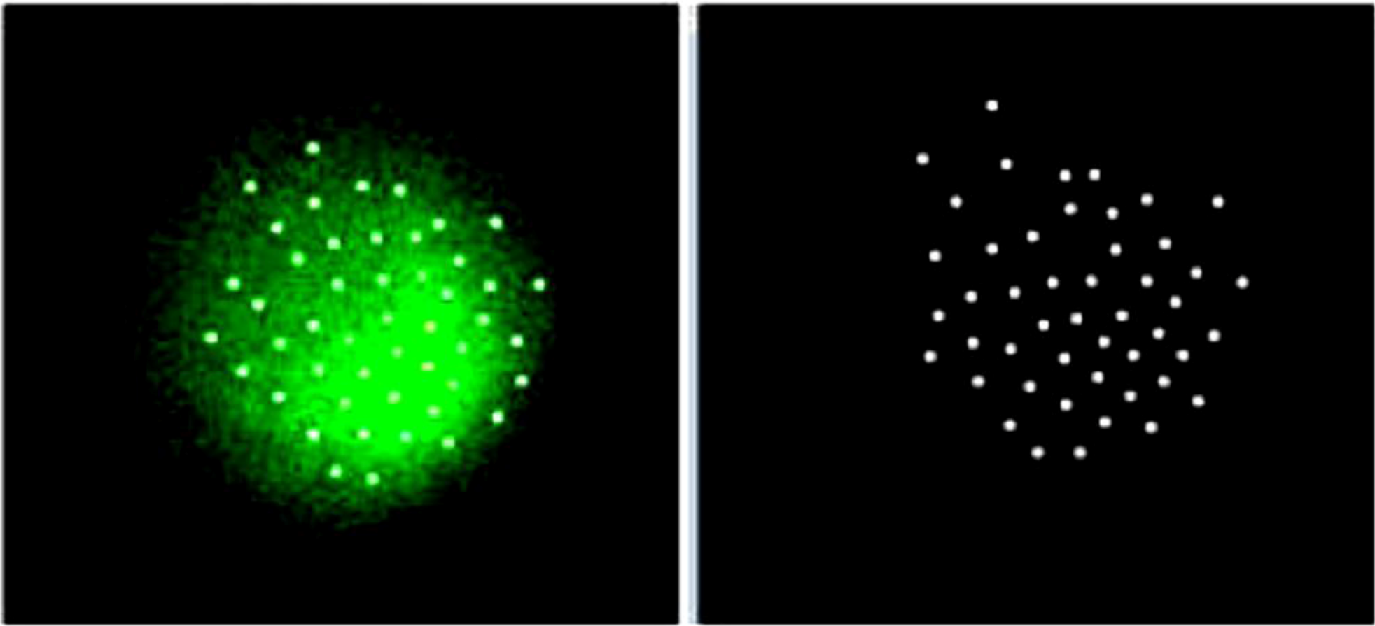
Figure 4.
Simulated Arena with double peak Gaussian distributed agents (a); Double peak shaped distribution of pollutant (b).
Figure 4.
Simulated Arena with double peak Gaussian distributed agents (a); Double peak shaped distribution of pollutant (b).
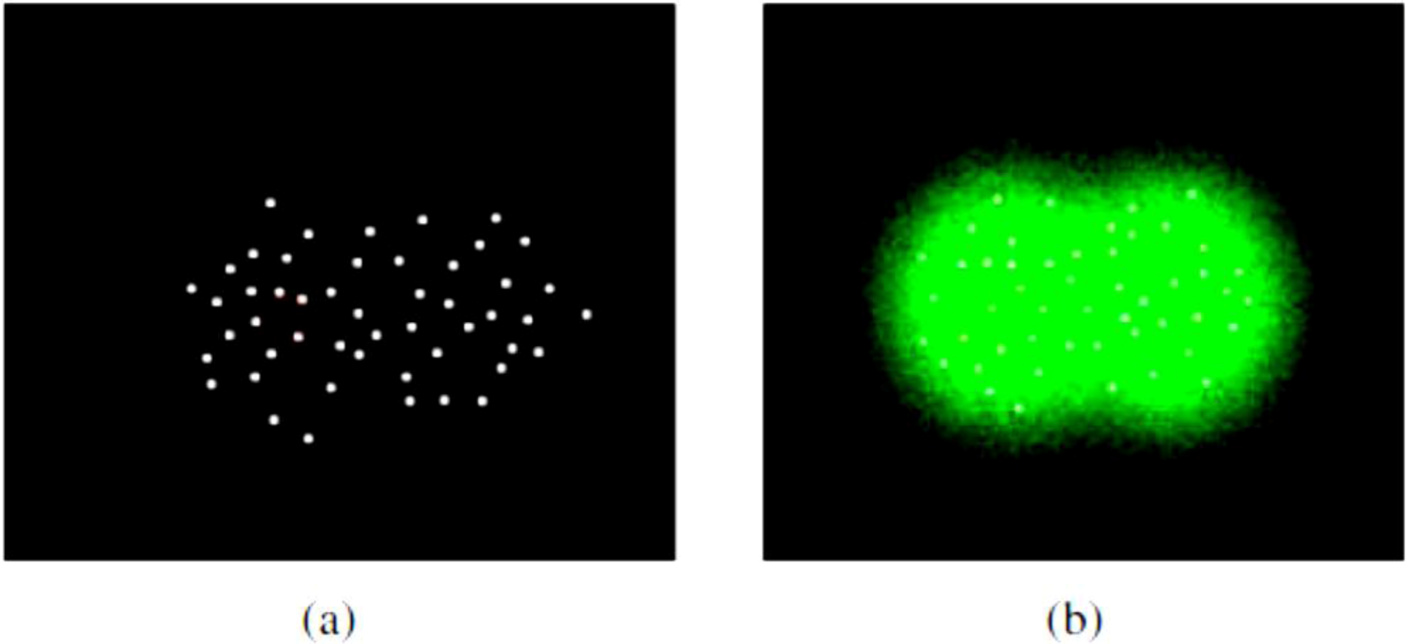
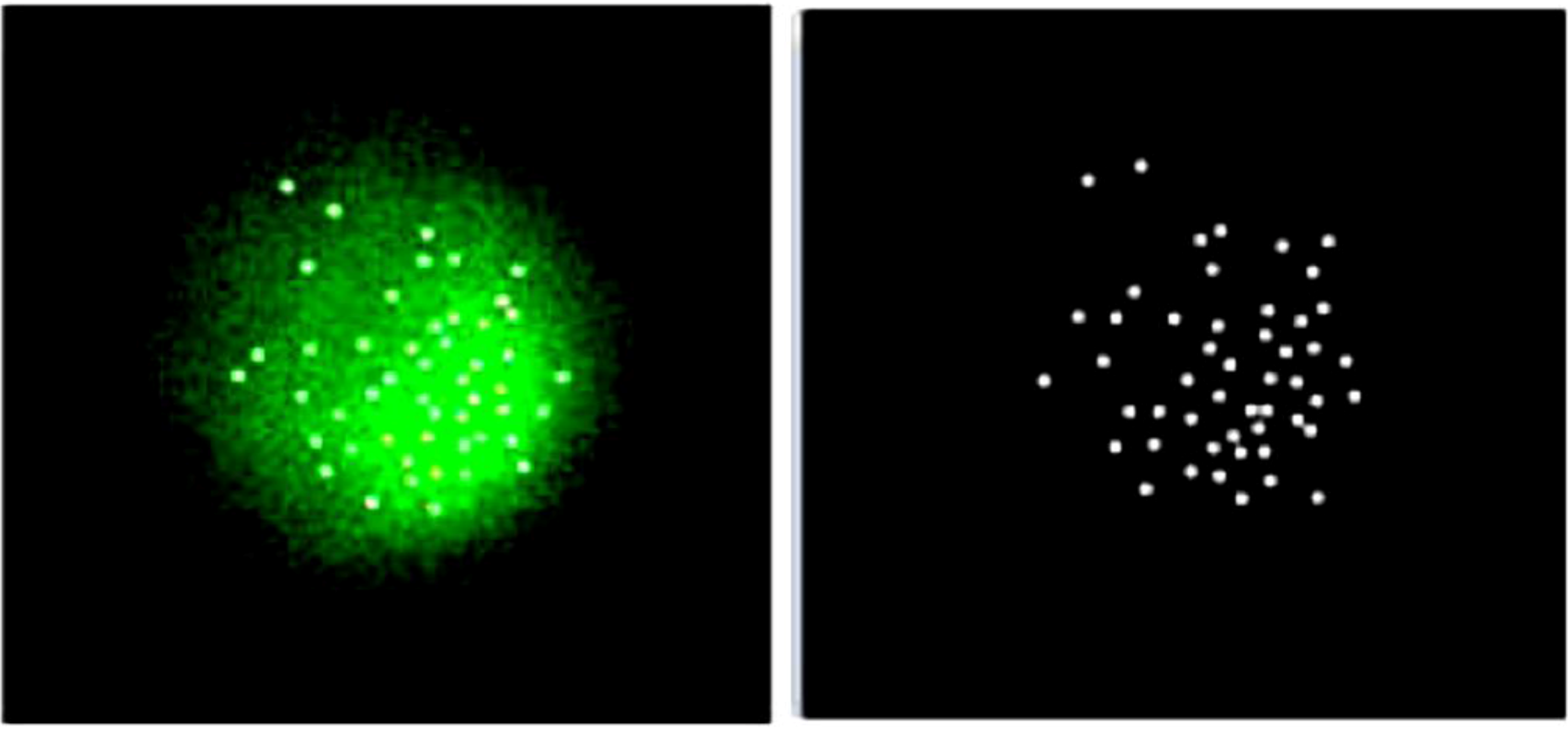
Figure 5.
Simulated Arena with doughnut shaped distribution of agents (a); Doughnut shaped distribution of pollutant (b).
Figure 5.
Simulated Arena with doughnut shaped distribution of agents (a); Doughnut shaped distribution of pollutant (b).
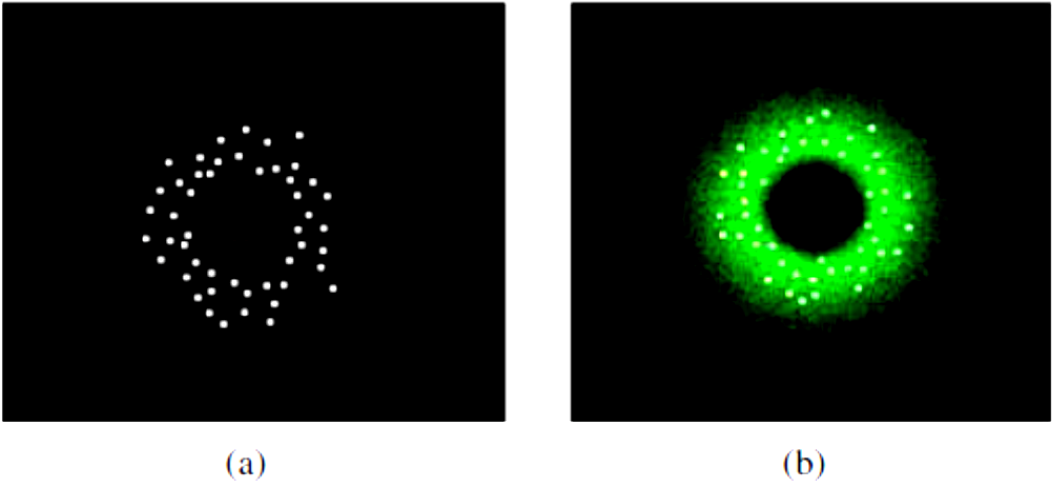
Figure 6.
Simulated Arena with squared shaped distribution of agents (a); Square shaped distribution of pollutant (b).
Figure 6.
Simulated Arena with squared shaped distribution of agents (a); Square shaped distribution of pollutant (b).
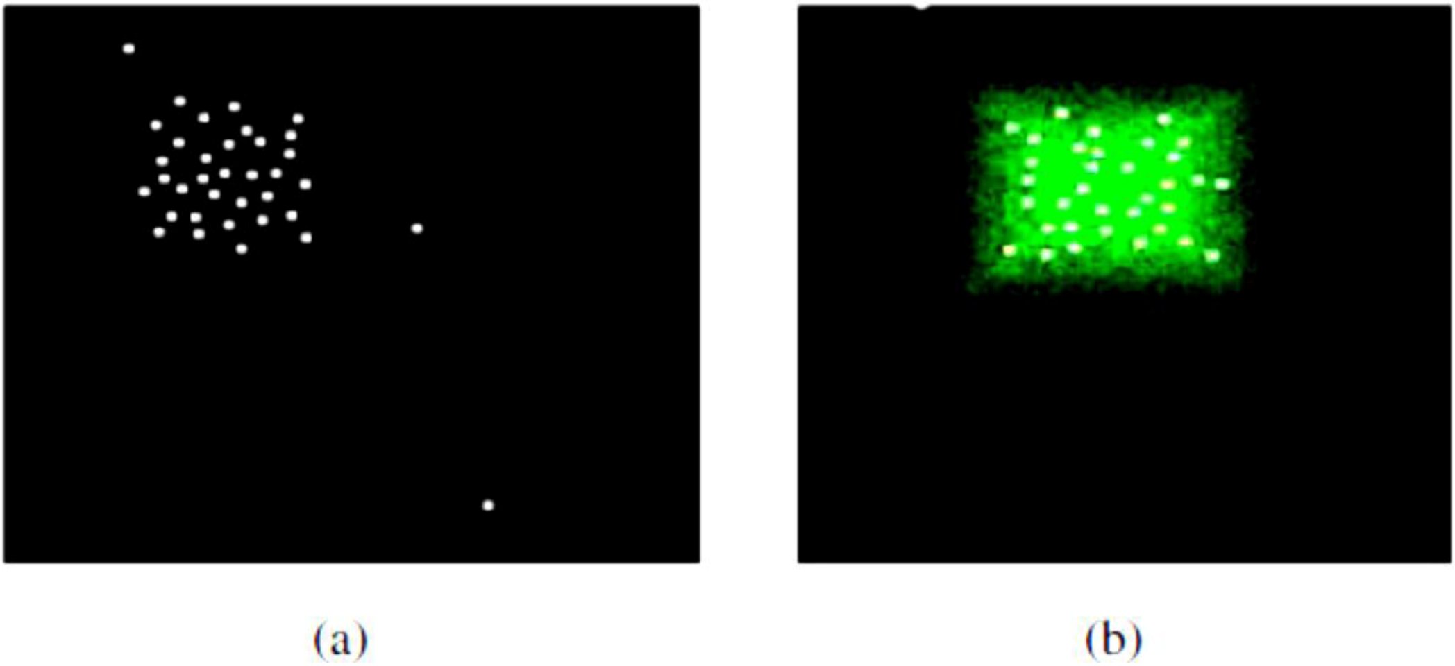
Figure 7.
Showing how the robots are distributed in a simulated skewed Gaussian profile using vk = 32.
Figure 7.
Showing how the robots are distributed in a simulated skewed Gaussian profile using vk = 32.

Figure 8.
Showing how the robots are distributed in a simulated skewed Gaussian profile using vk = 64.
Figure 8.
Showing how the robots are distributed in a simulated skewed Gaussian profile using vk = 64.
However, as choosing the right vk value is presently guess work, a way of using machine learning to do this can be investigated. The approach used in this paper relies on using a Genetic Algorithm based on Gaussian models. In order to do this, some modifications are made to Equation (7) as shown in Equation (9):
![Robotics 02 00001 i009]() where T can be viewed as a system temperature constant and can be used for tuning the system using an adaptable scheme.
where T can be viewed as a system temperature constant and can be used for tuning the system using an adaptable scheme.

By adjusting this constant, the spread of the agents in the environment could be controlled to achieve different effects. βi(t) is a dynamic velocity of agent i that depends on the present reading Ci(t) of the environmental quantity, ![Robotics 02 00001 i022]() is the standard velocity without any reading. This velocity function was embedded in the bacteria controller. The present reading Ci(t) of the agent adapts the velocity of the agent so that in an area of higher concentration, it moves slowly covering a smaller area and vice versa. How this achieves coverage can be explained using
is the standard velocity without any reading. This velocity function was embedded in the bacteria controller. The present reading Ci(t) of the agent adapts the velocity of the agent so that in an area of higher concentration, it moves slowly covering a smaller area and vice versa. How this achieves coverage can be explained using
![Robotics 02 00001 i010]() where Ai is the area covered by agent i, τ is the mean run time or mean run length of the bacteria controller and A = πτ2 is the area covered by the agent when the bacteria controller is tuned so that the agents motion is circular. As the agents get closer to the source, the area covered by them decreases due to a lower velocity and higher concentration reading while they cover a larger area if they have a higher velocity due to a lower concentration. The area covered by the pollutant is covered if the individual areas are covered by the agents as follows:
where Ai is the area covered by agent i, τ is the mean run time or mean run length of the bacteria controller and A = πτ2 is the area covered by the agent when the bacteria controller is tuned so that the agents motion is circular. As the agents get closer to the source, the area covered by them decreases due to a lower velocity and higher concentration reading while they cover a larger area if they have a higher velocity due to a lower concentration. The area covered by the pollutant is covered if the individual areas are covered by the agents as follows:
![Robotics 02 00001 i011]()
 is the standard velocity without any reading. This velocity function was embedded in the bacteria controller. The present reading Ci(t) of the agent adapts the velocity of the agent so that in an area of higher concentration, it moves slowly covering a smaller area and vice versa. How this achieves coverage can be explained using


This could be used to develop a control law as in Equations (12) and (13) if an estimate of the pollutant profile F(S(x)) in the environment S(x) were known and used to tune the system temperature T so that the spread of the agents in the environment is controlled. As a result, Equation (9) becomes Equation (14).
![Robotics 02 00001 i012]()
![Robotics 02 00001 i013]()
![Robotics 02 00001 i014]() where γ is an integral gain and
where γ is an integral gain and ![Robotics 02 00001 i023]() is a proportional gain. A Gaussian model based Genetic algorithm explained in Section 3 was used to estimate parameters of the pollutant profile F(S(x)) locally. The standard deviation parameters of the locally estimated Gaussian are then used in Equation (12) so that it becomes
is a proportional gain. A Gaussian model based Genetic algorithm explained in Section 3 was used to estimate parameters of the pollutant profile F(S(x)) locally. The standard deviation parameters of the locally estimated Gaussian are then used in Equation (12) so that it becomes
![Robotics 02 00001 i015]() where AT (x)std is the standard deviation of the flock positions. From machine learning, combination of Gaussian curves could be used to form various functions [43] so that the agents using the present approach are able to form various complex pollutant shapes. By using machine learning, it is possible to correctly get the shape of the pollutant and increase the rate of convergence. The disadvantage however is that the kernel function used to estimate the pollutant profile must be capable of forming the distribution of the pollutant profile effectively. Investigating the use of machine learning in improving the proposed control system opens up the possibility of studying how various real world conditions could affect the agents’ distribution. This knowledge can then be incorporated into the control system so that the flock of agents are better prepared to deal with the environmental conditions as they arise.
where AT (x)std is the standard deviation of the flock positions. From machine learning, combination of Gaussian curves could be used to form various functions [43] so that the agents using the present approach are able to form various complex pollutant shapes. By using machine learning, it is possible to correctly get the shape of the pollutant and increase the rate of convergence. The disadvantage however is that the kernel function used to estimate the pollutant profile must be capable of forming the distribution of the pollutant profile effectively. Investigating the use of machine learning in improving the proposed control system opens up the possibility of studying how various real world conditions could affect the agents’ distribution. This knowledge can then be incorporated into the control system so that the flock of agents are better prepared to deal with the environmental conditions as they arise.


 is a proportional gain. A Gaussian model based Genetic algorithm explained in Section 3 was used to estimate parameters of the pollutant profile F(S(x)) locally. The standard deviation parameters of the locally estimated Gaussian are then used in Equation (12) so that it becomes

3. Pollution Distribution Estimation Using Genetic Algorithm
Genetic Algorithm was used to approximate the distribution F(S(x)) of the pollution in the environment. As the proposed approach is aimed at use in an environment that is dominated by diffusion, we assume that a pollutant can be described using a Gaussian function. This can be explained by observing the behaviour of a drop of ink put into water. It starts out concentrated at the source point and as time progresses, the concentration at the source point will reduce while the surrounding areas become contaminated. This is as a result of diffusion.
This behaviour can be viewed as a Gaussian function of which amplitude at the source reduces from an initial value A to a stationary value Astationary as time t goes to infinity (A ➔ Astationary as t ➔ ∞) while the standard deviation σ becomes wider and goes to a stationary value σstationary as time t progresses to infinity (σ ➔ σstationary as t ➔ ∞). This can be modelled as in Equations (16) and (17). Where k1 is the rate of decay of the amplitude At at time t and k2 is a constant that can be used to tune the conversation of the change in amplitude to the spread of the pollutant.
![Robotics 02 00001 i016]()
![Robotics 02 00001 i017]()


3.1. Estimating Simple Gaussian Functions
In this work, a very slow (near negligible) diffusion was assumed. The Genetic Algorithm was used to estimate the parameters (amplitude, source location, and standard deviation) of a Gaussian function that was used to simulate the pollutant. The estimated standard deviation F(S(x))std was fed back to the robotic flock according to Equations (15), (13) and (14) in order to adjust the velocity of the agents to achieve optimal coverage of the environment.
The Genetic Algorithm was designed with 35 genes on each chromosome, with 7 genes representing each of the Gaussian’s amplitude, x and y standard deviations, and x and y means. Each gene could take a value of either 0 or 1. As a result, the estimation range for each of the parameter using the Genetic Algorithm was between 0 to 128. A gene pool size of 400 chromosomes, tournament size of 10, crossover, mutation, reproduction ratios of 10%, 75% and 15% were used respectively with 10 generations per run.
During simulation runs, agents explored the environment using both the bacteria and flocking algorithm whilst collecting spatial pollutant data. The spatial pollutant data was stored in a running memory having n = 20 elements. This data was then passed to the Genetic Algorithm in order to estimate the pollutant parameters.
3.2. Estimating Multi-Modal Gaussian Functions
A pollutant is known to break up into pieces due to the turbulent nature of the environment. Hence, the pollutant’s profile becomes one made up of various local maximums and one global maximum. This could also be viewed as noise. Nevertheless, the aim of the method proposed in this paper is to represent a pollutant’s profile as closely as possible. This would be a problem for the method discussed in Section 3.1 as it would attempt to estimate a single global estimate from the data collected by the agents.
In order to solve this problem, it is assumed that each agent i transmits its individual estimated Gaussian parameter values to its local neighbours j ∈ {1…N} present within an l = 5 units radius together with its position xi. A reduced communication radius value ensures that only local agents to a local maximum contribute to each other’s estimation.
Based upon this information, each agent uses an averaging scheme depicted by Equation (18) to reach a consensus as to the parameter values of the local maximum.
The consensus scheme works by using a weighted averaging mechanism so that values closer to what an individual agent i is estimating are given more weight than the values farther from its estimation:
![Robotics 02 00001 i018]() where kavei is the k-average of the parameters estimate by agent i, G(||.||) is a Gaussian curve with agent i’s estimate as the centre value, N is the number of agents in the neighbourhood of agent i. N ≥ 5 as this is used to simulate the communication limitation of the agent i in that it can only buffer up to five readings.
where kavei is the k-average of the parameters estimate by agent i, G(||.||) is a Gaussian curve with agent i’s estimate as the centre value, N is the number of agents in the neighbourhood of agent i. N ≥ 5 as this is used to simulate the communication limitation of the agent i in that it can only buffer up to five readings.

By using the parallelism offered by swarm robotics and the consensus scheme as discussed above, it is possible to obtain an estimation of the pollutant’s profile in addition to recovering the function representing it.
The overall structure of the algorithm can be presented as in Algorithm 1. Lines four to six are necessary for a moving or changing pollutant profile. This has been tested in simulations with satisfactory results. The use of the model based genetic algorithm with the previous architecture is shown in Figure 9.

| run bacteria and flocking controller |
| collect data from environment and neighbours |
| update counter |
| if counter > noOfRuns then |
| Use GA to estimate model |
| end if |
| use GA estimates to update velocity function. |
Figure 9.
Architecture of the coverage controller using model based genetic algorithm.

4. Simulation and Results
4.1. Simple Gaussian Functions
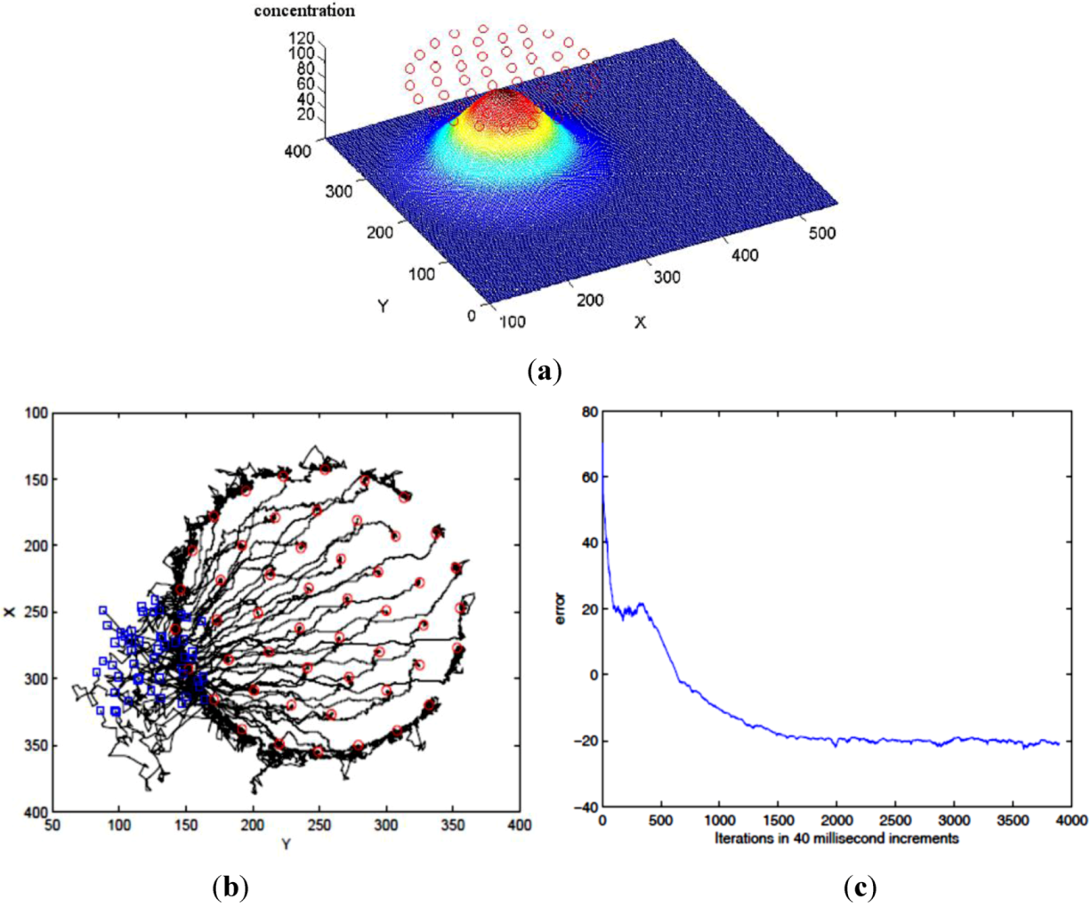
In order to test the approach, different pollutant profiles were generated with 50 agents deployed. A Gaussian having the following parameters of mean (x, y) = (400, 200), spread (x, y) = (38, 38) and amplitude of 100 was used. As can be seen in Figure 10, the agents were able to form the distribution even though their motion from Figure 10(b) seems erratic. This behaviour is as a result of the bacteria controller searching for a favourable path towards the optimal of the Gaussian distribution. Figure 10(c) shows how the error between the agents spread and the pollution spread reduces with time. The error was obtained by using Equation (14).
Figure 10.
Robots forming a Gaussian distribution. The blue squares are the deployment points while the red dots are the end points of the agents.
Figure 10.
Robots forming a Gaussian distribution. The blue squares are the deployment points while the red dots are the end points of the agents.

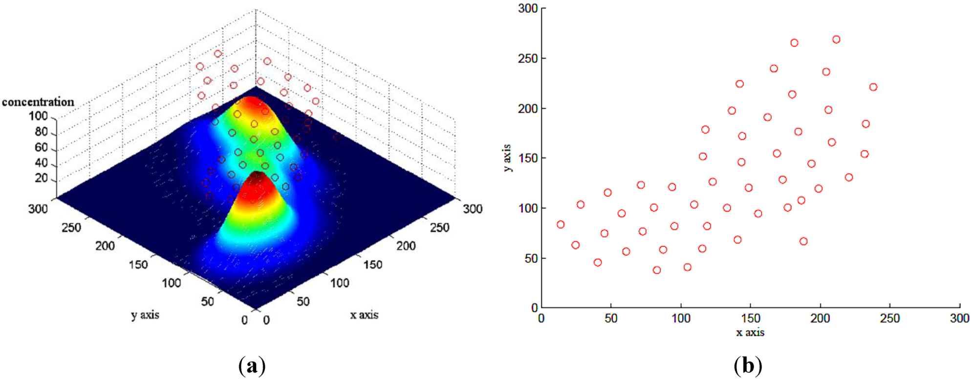
Figure 11.
Robots forming a distribution of three Gaussian distributions having means (x, y) = (80, 70), (170, 150), (200, 200), spreads (x, y) = (60, 40), (30, 80), (40, 80) and Amplitudes 100, 45, and 80 respectively.
Figure 11.
Robots forming a distribution of three Gaussian distributions having means (x, y) = (80, 70), (170, 150), (200, 200), spreads (x, y) = (60, 40), (30, 80), (40, 80) and Amplitudes 100, 45, and 80 respectively.

Another simulated pollutant profile generated by adding three Gaussian functions of randomly chosen parameters: means (x, y) = (80, 70), (170, 150), (200, 200), spreads (x, y) = (60, 40), (30, 80), (40, 80) and amplitudes = 100, 45 and 80 respectively were used as in Figure 11. It was observed that the approach enabled the agents to distribute according to the simulated pollutant’s profile.
4.2. Multi-Modal Gaussian Function
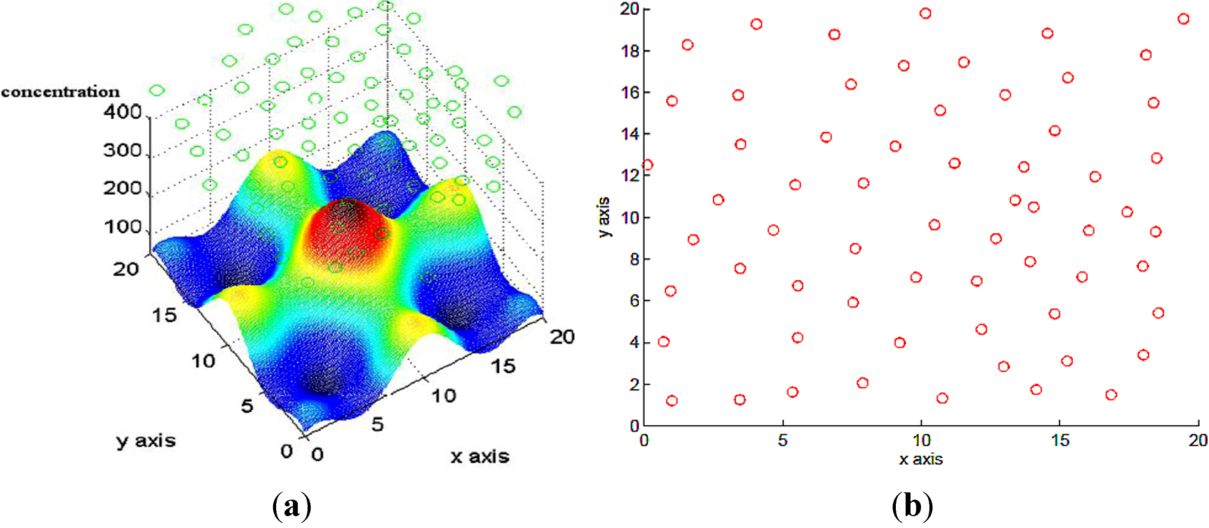
Using the approach discussed in Section 3.2, tests on multimodal Gaussian functions generated by C = 160+ (x2 – 150cos(2πxP1) + y2 – 150cos(2πyP2)) were carried out with P1 = P2 = 0.065. During these experiments, 100 agents were deployed with sensor readings for the agents normalized between the ranges of 0 to 100 as that is the range that the Genetic Algorithm was designed to handle. A higher number of agents were deployed because of the nature of the pollutant profile.
As can be observed in Figure 12, 60 of the agents were able of form the shape of the pollutant to a limited extent with the dips in the multimodal function seen in the agents distribution at (x, y) = (2.5, 16) and (x, y) = (15, 16). The rest of the agents were exploring the environment.
Figure 12.
Robots forming a distribution of a complex multimodal function having global maximum (x, y) = (10, 10).
Figure 12.
Robots forming a distribution of a complex multimodal function having global maximum (x, y) = (10, 10).
5. Conclusion
As discussed in the introduction of this paper, this work consisted of two parts: the first part uses a swarm of robots to provide a visual representation of a noisy static pollutant. For this, the method in this work relied on using the bacterium behaviour, flocking behaviour, and a velocity function. However, this part relied on choosing an appropriate value for vk in the velocity function. It was shown that the proposed method could be classified into the ant robotics category due to its limited communication capability, memory, and computational requirement. As a result, according to present knowledge, this is one of the first pieces of work that use ant robotics to create a visual representation of an invisible pollutant.
The second part of this work is the development of a feedback system that used the error between the standard deviation of the swarm member positions and the pollutant profile to choose an appropriate value for vk. The standard deviation of the pollutant profile was estimated by using a computationally efficient model based Genetic Algorithm that relied on the parallelism offered by the swarm to reach a consensus among swarm members when the pollutant profile became more challenging.
However, the implementation of Genetic Algorithm takes the agents out of the scope of ant robotics because of the amount of memory elements that would be required to store the gene pool alone. In addition, noise would adversely affect the estimation of the Genetic Algorithm which raises the question of whether an alternative scheme that is less affected by noise can be developed. A cooling scheme borrowed from the theory of Simulated Annealing might offer promising results and this would be the task of future investigations.
Other areas to be investigated include: Estimating swarm convergence time to a pollutant profile and studying the effect of dynamic cleaning of the pollutant on the proposed approach upon encounter.
Acknowledgments
This research work was financially supported by European Union FP7 program, ICT-231646, SHOAL, and the UK EPSRC Global Engagements grant EP/K004638/1.
References
- Ramana, M.V.; Ramanathan, V.; Kim, D.; Roberts, G.C.; Corrigan, C.E. Albedo, atmospheric solar absorption and heating rate measurements with stacked UAVs. Quart. J. Roy. Meteorol. Soc. 2007, 133, 1913–1931. [Google Scholar] [CrossRef]
- Giudice, A.G.; Melita, L.C.D.; Orlando, M.A. An overview of the “Volcan Project”: An UAS for exploration of volcanic environments. In Unmanned Aircraft Systems; Springer: Berlin, Germany, 2009; pp. 471–494. [Google Scholar]
- Puzis, R.; Altshuler, Y.; Elovici, Y.; Bekhor, S.; Shiftan, Y.; Pentland, A. Augmented Betweenness Centrality for Environmentally-Aware Traffic Monitoring in Transportation Networks. Available online: http://web.media.mit.edu/~yanival/JITS-environmental.pdf (accessed on 8 November 2012).
- Cortes, J.; Martinez, S.; Karatas, T.; Bullo, F. Coverage control for mobile sensing networks. IEEE Trans. Robotics Automat. 2004, 20, 243–255. [Google Scholar] [CrossRef]
- Schwager, M.; Slotine, J.; Rus, D. Consensus Learning for Distributed Coverage Control. In Proceedings of International Conference on Robotics and Automation, Pasadena, CA, USA, 19–23 May 2008; pp. 1042–1048.
- Schwager, M.; Mclurkin, J.; Slotine, J.E.; Rus, D. From theory to practice: Distributed coverage control experiments with groups of robots. Springer Tracts Adv. Robotics 2009, 54, 127–136. [Google Scholar] [CrossRef]
- Cortez, R.A.; Tanner, H.G.; Lumia, R. Distributed robotic radiation mapping. Springer Tracts Adv. Robotics 2009, 54, 147–156. [Google Scholar] [CrossRef]
- Pimenta, L.C.A.; Schwager, M.; Lindsey, Q.; Kumar, V.; Rus, D.; Mesquita, R.C.; Pereira, G.A.S. Simultaneous coverage and tracking (SCAT) of moving targets with robot networks. Springer Tracts Adv. Robotics 2010, 8, 1–16. [Google Scholar]
- Schwager, M.; Slotine, J.; Rus, D. Decentralized, Adaptive Control for Coverage with Networked Robots. In Proceedings of IEEE International Conference on Robotics and Automation, Roma, Italy, 10–14 April 2007; pp. 3289–3294.
- Shucker, B.; Murphey, T.; Bennett, J.K.; Member, S. Convergence preserving switching for topology dependent decentralized systems. IEEE Trans. Robot. 2008, 24, 1–11. [Google Scholar] [CrossRef]
- Shucker, B.; Murphey, T.; Bennett, J.K. An Approach to Switching Control beyond Nearest Neighbor Rules. In Proceedings of American Control Conference, Minneapolis, MN, USA, 14–16 June 2006.
- Kwok, A.; Martinez, S. A Distributed Deterministic Annealing Algorithm for Limited-Range Sensor Coverage. In Proceedings of American Control Conference, St. Louis, MI, USA, 10–12 June 2009; pp. 1448–1453.
- Pang, S.; Farrell, J.A. Chemical plume source localization. IEEE Trans. Syst. Man Cybern. B Cybern. 2006, 36, 1068–1080. [Google Scholar] [CrossRef]
- Koenig, S. Terrain Coverage with Ant Robots: A Simulation Study. In Proceedings of the International Conference on Autonomous Agents, Montreal, Canada, 28 May–1 June 2001; pp. 600–607.
- Koenig, S.; Szymanski, B.; Liu, Y. Efficient and inefficient ant coverage methods. Ann. Math. Artif. Intell. 2001, 31, 41–76. [Google Scholar]
- Wagner, I.A.; Altshuler, Y.; Yanovski, V.; Bruckstein, A.M. Cooperative cleaners: A study in ant robotics. Int. J. Robot. Res. 2008, 27, 127–151. [Google Scholar] [CrossRef]
- Altshuler, Y.; Yanovsky, V.; Wagner, I.A.; Bruckstein, A.M. Swarm Robotics for a Dynamic Cleaning Problem. In Proceedings of the IEEE Swarm Intelligence Symposium, Pasadena, CA, USA, June 2005; pp. 1–14.
- Altshuler, Y.; Bruckstein, A.M. Static and expanding grid coverage with ant robots: Complexity results. Theor. Comput. Sci. 2011, 412, 4661–4674. [Google Scholar] [CrossRef]
- Borie, R.; Tovey, C. Algorithms and Complexity Results for Pursuit-Evasion Problems. In Proceedings of the Twenty-First International Joint Conference on Artificial Intelligence, Pasadena, CA, USA, 11–17 July 2009; pp. 59–66.
- Arkin, R.C. Behaviour-Based Robotics; The MIT Press: Cambridge, MA, USA, 1998. [Google Scholar]
- Schwager, M.; Slotine, J.; Rus, D. Unifying Geometric, Probabilistic, and Potential Field Approaches to Multi-Robot Coverage Control. In Proceedings of the International Symposium on Robotics Research, Lucerne, Switzerland, 31 August–3 September 2009.
- Oyekan, J.; Hu, H.; Gu, D. A Novel Bio-Inspired Distributed Coverage Controller for Pollution Monitoring. In Proceedings of the 2011 IEEE International Conference on Mechatronics and Automation, Beijing, China, 7–10 August 2011; pp. 1651–1656.
- Baronov, D.; Baillieul, J. Autonomous Vehicle Control for Ascending/Descending along a Potential Field with Two Applications. In Proceedings of the American Control Conference, Seattle, WC, USA, 11–13 June 2008; pp. 678–683.
- Mayhew, C.G.; Sanfelice, R.G.; Teel, A.R. Robust Source-Seeking Hybrid Controllers for Nonholonomic Vehicles. In Proceedings of the American Control Conference, Seattle, WC, USA, 11–13 June 2008; pp. 2722–2727.
- Dhariwal, A.; Sukhatme, G.S.; Requicha, A.A.G. Bacterium-Inspired Robots for Environmental Monitoring. In Proceedings of IEEE International Conference on Robotics and Automation, New Orleans, LA, USA, 26 April–1 May 2004; pp. 1436–1443.
- Marques, L.; Nunes, U.; Almeida, T.D. Olfaction-based mobile robot navigation. Thin Solid Films 2002, 418, 51–58. [Google Scholar]
- Lilienthal, A.; Duckett, T. Experimental Analysis of Smelling Braitenberg Vehicles. In Proceedings of IEEE International Conference on Advanced Robotics, Coimbra, Portugal, 30 June–3 July 2003; pp. 375–380.
- Brown, D.A.; Berg, H.C. Temporal stimulation of chemotaxis in Escherichia coli. Proc. Natl. Acad. Sci. USA 1974, 71, 1388–1392. [Google Scholar]
- Yi, T.; Huang, Y.; Simon, M.; Doyle, J. Robust perfect adaptation in bacterial chemotaxis through integral feedback control. Proc. Natl. Acad. Sci. 2000, 97, 4649–4653. [Google Scholar]
- Berg, H.C.; Purcell, E.M. Physics of chemoreception. Biophys. J. 1977, 20, 193–219. [Google Scholar]
- Oyekan, J.; Hu, H. Bacteria Controller Implementation on a Physical Platform for Pollution Monitoring. In Proceedings of IEEE International Conference on Robotics and Automation, Anchorage, AK, USA, 3–8 May 2010; pp. 3781–3786.
- Oyekan, J.O.; Hu, H.; Gu, D. Bio-inspired coverage of invisible hazardous substances in the environment. Int. J. Inform. Acquis. 2010, 7, 193–204. [Google Scholar]
- Oyekan, J.; Gu, D.; Hu, H. Hazardous Substance Source Seeking in a Diffusion Based Noisy Environment. In Proceedings of the 2012 IEEE International Conference on Mechatronics and Automation, Sichuan, China, 5–8 August 2012; pp. 708–713.
- Oyekan, J.; Gu, D.; Hu, H. Visual imaging of invisible hazardous substances using bacterial inspiration. IEEE Trans. Syst. Man Cybern. Syst. Hum. 2013, in press. [Google Scholar]
- Hamann, H.; Heinz, W. A framework of space-time continuous models for algorithm design in swarm robotics. Swarm Intelligence 2008, 2, 209–239. [Google Scholar]
- Schweitzer, F. Brownian Agent Models for Swarm and Chemotactic Interaction Brownian Agents. In Proceedings of the Fifth German Workshop on Artificial Life, Lübeck, Germany, 12–18 March 2002; pp. 181–190.
- Reynolds, C.W. Flocks, Herds and Schools: A Distributed Behavioral Model. In Proceedings of the 14th Annual Conference on Computer Graphics and Interactive Techniques, New York, NY, USA, July 1987; Volume 21, pp. 25–34.
- Hanay, Y.S.; Ilter, M. Aggregation, Foraging, and Formation Control of Swarms with Non-Holonomic Agents Using Potential Functions and Sliding Mode Techniques. In Proceedings of European Control Conference (ECC 2007), Kos, Greece, 2–5 July 2007; Volume 15, pp. 149–168.
- Gazi, V. Coordination and Control of Multi-Agent Dynamic Systems: Models and Approaches. In Proceedings of the 2nd International Conference on Swarm Robotics (SAB ’06), Rome, Italy, 30 September 30–1 October 2006; pp. 71–102.
- Olfati-saber, R. Flocking for multi-agent dynamic systems: Algorithms and theory. IEEE Trans. Automat. Contr. 2006, 54, 401–420. [Google Scholar]
- Smith, J.A. Comparison of Hard-Core and Soft-Core Potentials for Modelling Flocking in Free Space. Available online: http://arxiv.org/abs/0905.2260 (accessed on 8 November 2012).
- Oyekan, J.; Hu, H.; Gu, D. Exploiting Bacterial Swarms for Optimal Coverage of Dynamic Pollutant Profiles. In Proceedings of the IEEE International Conference on Robotics and Biomimetics, Tianjin, China, 14–18 December 2010; pp. 1692–1697.
- Sanner, R.; Slotine, J.J. Gaussian networks for direct adaptive control. IEEE Trans. Neural Networks 1992, 3, 837–863. [Google Scholar]
© 2013 by the authors; licensee MDPI, Basel, Switzerland. This article is an open-access article distributed under the terms and conditions of the Creative Commons Attribution license (http://creativecommons.org/licenses/by/3.0/).
Share and Cite
MDPI and ACS Style
Oyekan, J.; Hu, H. Ant Robotic Swarm for Visualizing Invisible Hazardous Substances. Robotics 2013, 2, 1-18. https://doi.org/10.3390/robotics2010001
AMA Style
Oyekan J, Hu H. Ant Robotic Swarm for Visualizing Invisible Hazardous Substances. Robotics. 2013; 2(1):1-18. https://doi.org/10.3390/robotics2010001
Chicago/Turabian StyleOyekan, John, and Huosheng Hu. 2013. "Ant Robotic Swarm for Visualizing Invisible Hazardous Substances" Robotics 2, no. 1: 1-18. https://doi.org/10.3390/robotics2010001