Article

Computationally Efficient Adaptive Type-2 Fuzzy Control of Flexible-Joint Manipulators

by
Hicham Chaoui
1,
Wail Gueaieb
1,*,
Mohammad Biglarbegian
2 and
Mustapha C. E. Yagoub
1
1
School of Electrical Engineering and Computer Science, University of Ottawa, 800 King Edward Avenue, Ottawa, ON K1N 6N5, Canada
2
School of Engineering, University of Guelph, Guelph, ON N1G 2W1, Canada
*
Author to whom correspondence should be addressed.
Robotics 2013, 2(2), 66-91; https://doi.org/10.3390/robotics2020066
Submission received: 1 April 2013 / Revised: 4 May 2013 / Accepted: 13 May 2013 / Published: 21 May 2013
(This article belongs to the Special Issue Intelligent Robots)

Abstract

:
In this paper, we introduce an adaptive type-2 fuzzy logic controller (FLC) for flexible-joint manipulators with structured and unstructured dynamical uncertainties. Simplified interval fuzzy sets are used for real-time efficiency, and internal stability is enhanced by adopting a trade-off strategy between the manipulator’s and the actuators’ velocities. Furthermore, the control scheme is independent of the computationally expensive noisy torque and acceleration signals. The controller is validated through a set of numerical simulations and by comparing it against its type-1 counterpart. The ability of the adaptive type-2 FLC in coping with large magnitudes of uncertainties yields an improved performance. The stability of the proposed control system is guaranteed using Lyapunov stability theory.

Graphical Abstract

1. Introduction

Flexible-joint manipulators offer several advantages with respect to their rigid counterpart, such as light weight, lower cost, smaller actuators, larger work volume, better manoeuvrability and transportability, higher operational speed, power efficiency, and larger number of applications. Thus, they are often required to operate at high speed to yield high productivity. The conflicting requirements between high speed and high accuracy make the robotic control task a challenging research problem. Reducing the weight of the arms and/or increasing the operation speed make many industrial flexible-joint manipulators face arm vibration problems, particularly in high speed motion, because of the low stiffness. This can be resolved by increasing the stiffness. However, it increases the mass, depleting the advantages listed above. Typical challenges include severe friction nonlinearities, coupling stemming from the manipulator’s flexibility, varying operating conditions, structured and unstructured dynamical uncertainties, and external disturbances.
Flexibility and nonlinear friction may have some destabilizing effects when failing to compensate for modeling uncertainties in controlling flexible structures. These phenomena have been thoroughly studied in many control systems for high quality servomechanisms. Several studies show these negative consequences, such as severe tracking errors, limit cycles, chattering, and excessive noise [1,2]. Many control laws have been proposed for flexible joints [1,3,4], including classical, robust and adaptive control laws, using techniques such as singular perturbations and energy methods [5], but they generally consider (structured) parametric uncertainties only. Several models and compensation schemes have been proposed. Adaptive control techniques have been regarded among the most promising solutions to such type of problems. However, not much has been achieved yet for systems that exhibit both flexibility and severe nonlinearities.
Flexible-joint manipulators are governed by complex dynamics and hence controlling them depends on their dynamic models. There are many modeling techniques for mechanical systems, such as Lagrangian approach, Hamilton’s principle, and Kane method. Yet, the system is inevitably subjected to the ubiquitous presence of high, particularly unstructured, modeling nonlinearities, such as Coulomb friction and external disturbances. The presence of such uncertainties on a manipulator driven through a flexible joint significantly changes the system’s dynamics as opposed to when the load is driven with a rigid joint [6,7]. In this case, solving the inverse dynamics of the system is not realizable since the motor position is not uniquely defined at standstill. This last condition also illustrates that the actuator’s state cannot be observed continuously from the load output. Henceforth, only an approximate inverse model can be realized. Therefore, modeling the system’s dynamics based on presumably accurate mathematical models cannot be applied efficiently in this case. This raises the urgency to consider alternative approaches for the control of this type of manipulator systems to keep up with their increasingly demanding design requirements.
Various control techniques were proposed over the years to control flexible-joint manipulators [8,9,10]. De Luca et al. [11] and Khorasani [12] proposed feedback linearization-based controllers. However, these controllers depend on excessively noisy joint acceleration and jerk signal measurements and are hence unreliable in most real-world robotic systems. On the other hand, C. de Wit [13] proposed a robust control scheme for friction overcompensation due to uncertainties in friction models. Even as such, the suggested controllers require the full a priori knowledge of the system’s dynamics. This problem has been partially overcome by several adaptive control schemes [14,15,16]. Most of these control techniques capitalize on the singular perturbation theory to extend the adaptive control theory developed for rigid bodies to flexible ones [17,18,19,20]. M. Spong [21] reduced the flexible-joint manipulators model to the standard rigid manipulators model as the joint stiffness tends to infinity. This model has been widely used by many researchers to achieve better tracking performance. For example, F. Ghorbel et al. [5] used a rigid manipulator’s conventional method as slow controller and a fast feedback control law to damp out the oscillations of the joint flexibility modes. In a similar way, K. Khorasani et al. [22] illustrated how standard adaptive control schemes for rigid robots may be generalized for flexible-joint manipulators under a certain set of assumptions. Although many of these controllers are shown to be quite performant in theory, they failed to address important issues that might stand against their practical implementation, like basing the control laws on joint torques and their derivative [23,24], for instance, which are well known to be extremely noisy in real-life applications.
Moreover, such type of control algorithms uses online continuous estimation through well-defined adaptation laws of a set of the plant’s physical parameters to approximate the system’s dynamics. For it to provide a satisfactory performance, a typical adaptive control algorithm assumes that the dynamic model is perfectly known and free of significant external (unmodeled) disturbances. In other words, the controller is only robust to parametric or structured (also called modeled) uncertainties and possibly to minor unstructured uncertainties. Moreover, the unknown physical parameters must have constant or slowly varying nominal values. An explicit linear parameterization of the uncertain dynamics parameters also has to exist, and even if it does, it might not be trivial to derive, especially with complex dynamic systems. Although the latter condition is guaranteed for robotic systems, it might not be the case for many other dynamic models. Although some conventional adaptive control techniques, proposed in the literature, did indeed tackle external disturbance attenuation in addition to the compensation for parametric uncertainties, they did not take into consideration the effects of modeling uncertainties [14].
There is an increasing interest in developing new adaptive control schemes for robot manipulators [25,26]. For example, in [25] an adaptive neural network based sliding mode control was developed. The authors in [27] developed a neural network and an estimator to estimate the external perturbation on flexible robot manipulators. This work does not consider uncertainty in the robot parameters and was validated in simulations only. In another work, an adaptive based output-feedback control strategy for global position stabilization was developed in [28]. Although this work guarantees the adaptive regulation objective without the need for velocity feedback, it does not consider parameter uncertainties. A voltage-based adaptive control methodology for flexible joint manipulators was developed in [29,30]. The advantage of this work is that it is not torque-based control. However, it does not consider dynamic parameter uncertainties and was validated only in simulations.
In the literature, several papers on the robust control of robot manipulators have been developed, most of which use sliding mode techniques [31,32,33]. In [31] a multiple model/control strategy was proposed. It uses sliding mode control to reduce the high gain control for robot manipulators with large parameter uncertainty. In another work, a digital sliding mode controller for manipulators with three joints was developed by Corradini et al. [32]. This controller is not adaptive and uses sliding mode structure, which is prone to chattering.
On the other hand, computational intelligence tools, such as artificial neural networks and fuzzy logic controllers, have been credited in various applications as powerful tools capable of providing robust controllers for mathematically ill-defined systems that may be subjected to structured and unstructured uncertainties [34,35]. The universal approximation theorem has been the main driving force behind the increasing popularity of such methods as it shows that they are theoretically capable of uniformly approximating any continuous real function to any degree of accuracy. This has led to the recent advances in the area of intelligent control [36,37]. Various neural network and fuzzy logic models have been applied in the control of flexible joint manipulators, which have led to a satisfactory performance [9,10]. H. Chaoui et al. [38,39,40,41] used a neural network based adaptive control approach inspired by sliding mode control to learn the system’s dynamics. A time-delay neurofuzzy network was suggested in [42], where a linear observer was used to estimate the joint velocity signals and eliminated the need to measure them explicitly. Subudhi et al. [43] presented a hybrid architecture composed of a neural network to control the slow dynamic subsystem and an H to control the fast subsystem. A feedback linearization technique using a Takagi–Sugeno neurofuzzy engine was adopted in [44]. Despite the success witnessed by neural network-based control systems, they remain incapable of incorporating any human-like expertise already acquired about the dynamics of the system in hand, which is considered one of the main weaknesses of such soft computing methodologies. In another work, an adaptive neural network based sliding mode control was developed in citeSun-2011. However, only simulations were used to verify the results. Type-1 FLCs have also been developed for robot manipulators. Some of these control techniques have hybridized type-1 FLCs with sliding mode control to achieve good robustness; e.g., Li and Huang [45] developed an MIMO adaptive sliding mode based manipulator. However, only simulations were performed to validate the theory.
As type-2 FLCs can handle uncertainties more effectively than type-1 FLCs, they are becoming a more viable tool for the control of uncertain systems [46]. Melin and Castillo [47,48] reviewed genetic algorithms, particle swarm and ant colony optimization methods in the design of optimal type-2 fuzzy systems for different applications. The authors concluded that although genetic algorithms have been used more frequently, the other two methods are rapidly gaining ground for the design of optimum type-2 FLCs. The same authors adopted the chemical reaction algorithm (CRA) to tune the parameters of type-1 and type-2 FLCs for a unicycle tracking applications [49].
While several type-1 FLCs have been developed for robot manipulators [50], very few interval type-2 FLCs have been devised for this purpose [51,52,53]. In [52], a type-2 fuzzy controller was developed and tested on a parallel robot. Most recently, in [53], a type-2 TSK fuzzy controller was used to control a modular robot. Chen developed a sliding mode based type-2 FLC for trajectory tracking. The computational complexity of the hybrid controller is rather significant because of its learning structure. In all of these works, it was concluded that type-2 FLCs can outperform their type-1 counterparts despite noise and uncertainty.
The present work contributes to the merits and the latest developments of type-2 fuzzy logic theory for the design and implementation of an adaptive type-2 FLC for the control of flexible-joint robot manipulators with uncertain dynamics. The combination of high, particularly unstructured, nonlinearities, such as in the form of Coulomb friction, and manipulator’s joint elasticity changes significantly the system’s dynamics. In this case, the system’s inverse dynamic model cannot be found and only an approximation can be made. Therefore, modeling the system’s dynamics based on presumably accurate mathematical models cannot be applied efficiently in this case. Conventional type-1 fuzzy logic systems (FLSs) can be used to identify the behavior of this highly nonlinear system with various types of uncertainties. However, type-1 fuzzy sets may not fully capture the uncertainties in the system due to membership functions and knowledge base imprecision. Hence, higher types of fuzzy sets have to be considered. However, the computational complexity of operations on fuzzy sets increases with the increasing type of the fuzzy set. Therefore, interval type-2 fuzzy sets are adopted in this work for their simplicity and efficiency to capture the severe nonlinearities of flexible-joint robot manipulators. Thus far, type-2 FLSs have been used in very few control applications, such as nonlinear control and mobile robot navigation [54]. The work presented in this manuscript has two main contributions: (i) it devises a novel adaptive control law for type-2 FLCs; and (ii) it proposes a computationally efficient inference mechanism for such type of controllers, which are reputed for their typically high computational complexity, to make them more suitable for real-time applications. This work represents one of the scarce attempts in developing adaptive type-2 FLC to control flexible-joint manipulators with uncertain dynamics. To the best of our knowledge, adaptive type-2 FLCs with a Mamdani structure have not yet been developed for the control of robot manipulators. As shall be detailed later, and unlike other types of control systems proposed in the literature, the proposed adaptive type-2 FLC is proven to be stable by Lyapunov stability theory and does not depend on the excessively noisy acceleration signals or joint torque measures [23,24]. We also present a comparative study between the proposed adaptive type-2 FLC and its type-1 counterpart to better assess their respective performances in various operating conditions.
The rest of the paper is organized as follows: Section 2 outlines the dynamical model of a typical flexible-joint manipulator. In Section 3, an overview of type-2 fuzzy logic systems is presented. In Section 4, we present interval type-2 FLSs and describe the functionality of a type-2 fuzzy inference engine. The design of the proposed controller is detailed in Section 5. In Section 6, simulation results are reported and discussed before concluding the paper with a few remarks about this important, yet complex, control problem in Section 7.

2. Flexible-Joint Manipulator Dynamics

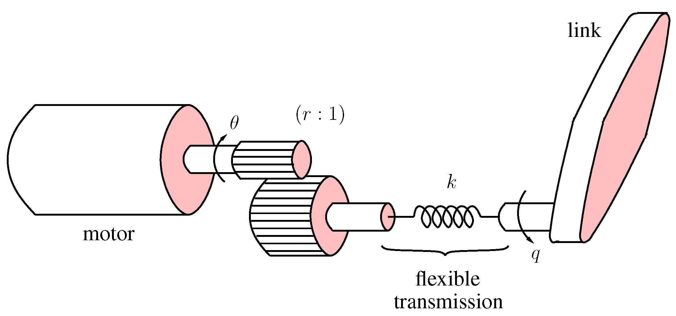
2.1. Modeling of a Flexible-Joint Manipulator

The schematic representation for the ith flexible-joint in a multi-joint manipulator is shown in Figure 1. The actuator is coupled to a flexible transmission through an r:1 reduction gear. The transmission is dynamically simplified as a linear torsional spring linked directly to the load (e.g., manipulator link.)
Figure 1. Flexible-joint model.
Robotics 02 00066 g001
Consider a robot manipulator with n revolute flexible joints. Using Euler–Lagrange formulation, the dynamic equations of the manipulator can be written as:
M ( q ) q ¨ + C ( q , q ˙ ) q ˙ + G ( q ) = τ t τ f l τ d l
J m θ ¨ = τ m 1 r τ t τ f m τ d m
τ t = K ( θ r q )
where,
q R n : vector of links’ positions θ R n : vector of motors’ positions M ( q ) R n × n : manipulator’s positive definite inertial matrix C ( q , q ˙ ) R n × n : matrix of Coriolis and centrifugal terms G ( q ) R n : vector of gravitational torques J m R n × n : motors’ diagonal inertial matrix τ t R n : vector of transmission torques τ m R n : motors’ generalized torque vector (control input) τ f l R n : load friction vector τ f m R n : motors’ friction vector τ d l R n : load’s unmodeled dynamics and external disturbance vector τ d m R n : motors’ unmodeled dynamics and external disturbance vector K R n × n : diagonal matrix of joints’ stiffness coefficients r R : gear ratio
The dynamics of a robotic manipulator is characterized by the following properties:
Property 1 
The inertia matrix M ( q ) is characterized by the following properties.
(1) 
Positive Definite Symmetric (PDS), i.e., M T ( q ) = M ( q ) and x T M ( q ) x > 0 for any non-null vector x.
(2) 
Upper and lower bounded, i.e., there exist two scalars α 1 ( q ) and α 2 ( q ) such that α 1 ( q ) I M ( q ) α 2 ( q ) I , where I is the identity matrix.
Property 2 
The Coriolis and centripetal term C ( q , q ˙ ) has the following properties.
(1) 
Matrix M ˙ ( q ) 2 C ( q , q ˙ ) is skew symmetric, i.e., x T ( M ˙ ( q ) 2 C ( q , q ˙ ) ) x = 0 x R n
(2) 
C ( q , q ˙ ) q ˙ is quadratic in q ˙ and bounded, i.e., there exists a scalar α 3 ( q ) such that C ( q , q ˙ ) q ˙ α 3 ( q ) q ˙ 2 .
Property 3 
The gravity vector G ( q ) is bounded, i.e G ( q ) α 4 ( q ) , for a scalar α 4 ( q ) .
Before we proceed further, we introduce the following realistic assumption.
Assumption 1 
The norm of the unknown disturbance τ d is upper bounded by a scalar b d , i.e., τ d b d .

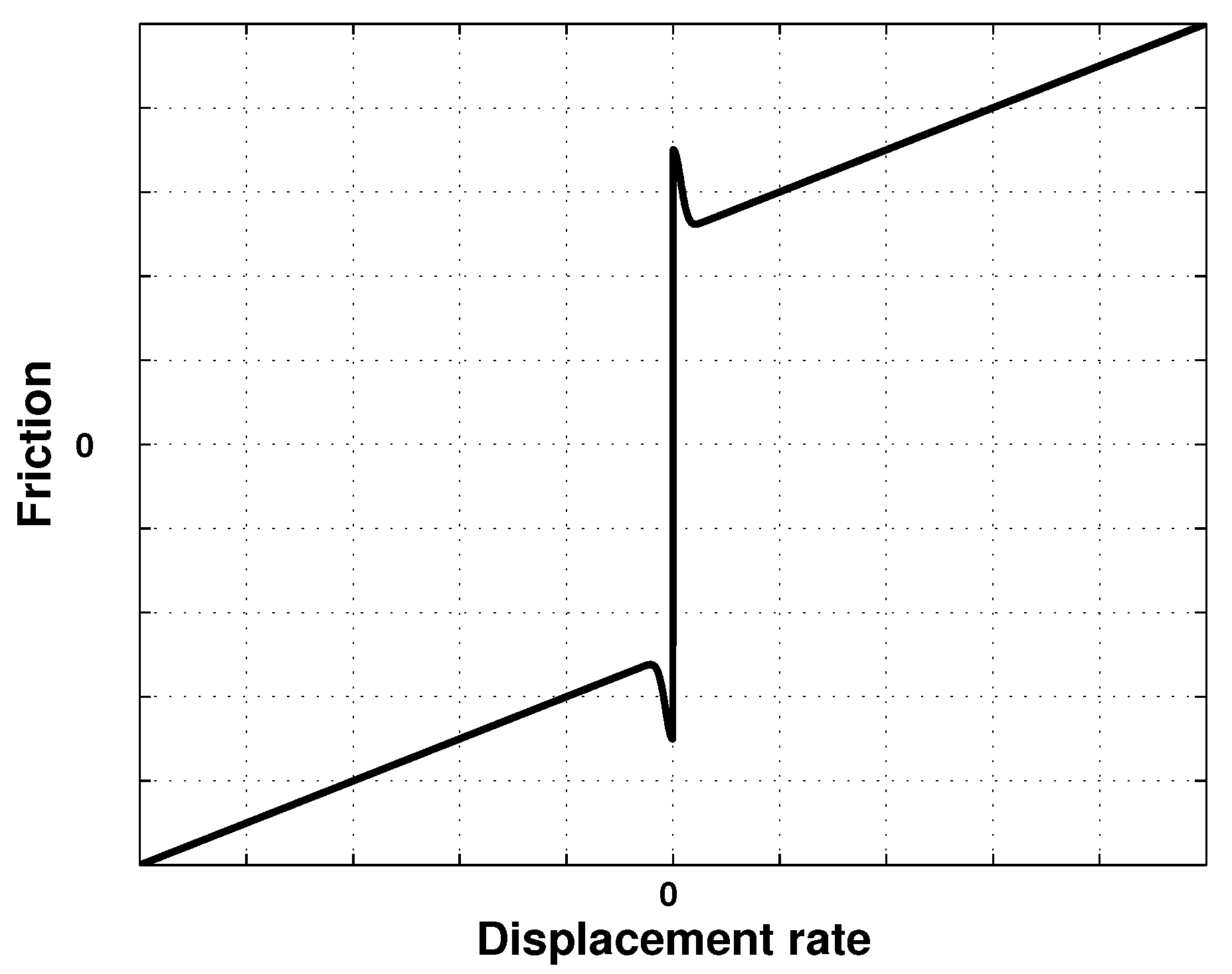
2.2. Friction Modeling

Friction is highly nonlinear and it is therefore important to capture the essence of the friction phenomena with models of reasonable complexity. The behavior of friction has been extensively examined lately, a good accurate representation was introduced in [4] as the sum of Coulomb, viscous, and static friction terms. The model of such a memoryless linear or angular friction F R n operating along a linear or angular displacement rate vector x ˙ = ( x ˙ 1 , , x ˙ n ) T R n can be expressed as
F ( x ˙ ) = F c sign ( x ˙ ) + F v x ˙ + F s Υ ( x ˙ ) sign ( x ˙ )
where F c = diag ( F c 1 , , F c n ) , F v = diag ( F v 1 , , F v n ) and F s = diag ( F s 1 , , F s n ) are the Coulomb, viscous and static friction positive definite diagonal matrices, respectively, and Υ ( x ˙ ) = diag ( e ( x ˙ 1 / η s 1 ) 2 , , e ( x ˙ n / η s n ) 2 ) is a positive definite diagonal matrix representing the rate of decay of the static friction for some decay rate scalars η s 1 , , η s n , along the n degrees of freedom. The term sign ( x ˙ ) R n is the vector ( sign ( x ˙ 1 ) , , sign ( x ˙ n ) ) T defined by
sign ( x ˙ i ) = 1 , if x ˙ i 0 1 , if x ˙ i < 0 , i = 1 , , n
Note the friction’s high sensitivity and nonlinearity in the vicinity of x ˙ = 0 , as illustrated in Figure 2. At very low velocity, manipulators are likely to exhibit undesirable stick-slip, a cycle of stop and motion. Friction will act as a constraint and not as a motion generator [55]. τ is the control input and ϵ is a very small constant.
Figure 2. Friction model.Friction
Robotics 02 00066 g002
In a single stage speed reduction system, a lumped flexibility model can be used if the dominant flexion appears in the gear teeth. In the following, the input gears inertia are combined with the actuators inertia J m while the output gears inertia is lumped with the load inertia M ( q ) . As shown in [38] and the references therein, this model reduction method has been used in multi-stage reduction systems, such as planetary gears, and in multi-mass flexibility models, like harmonic drives, for instance.

2.3. Problem Statement

Given the desired trajectories q d and q ˙ d , the aim is to design a control law τ m which ensures that the manipulator’s position q and velocity q ˙ track their desired trajectories under unknown or uncertain dynamics and in the presence of external disturbances. The proposed controller uses q, q ˙ , and θ ˙ as the system’s measurable states. The manipulator’s parameters, M ( q ) , C ( q , q ˙ ) , G ( q ) , J m , τ f l , τ f m , τ d l , τ d m are assumed to be unknown or uncertain.

3. Type-2 FLSs

A type-2 FLS is comprised of five components: fuzzifier, rule base, fuzzy inference engine, type-reducer and defuzzifier. A block diagram of a typical type-2 FLS is depicted in Figure 3.
Figure 3. Block diagram of a type-2 FLS.
Robotics 02 00066 g003
A type-2 fuzzy set is defined by a fuzzy membership function, where the membership value or grade for each element of this set is a fuzzy set in the interval [ 0 , 1 ] rather than a crisp value. As such, the footprint of uncertainty (FOU) provides type-2 FLSs with additional degrees of freedom, making the membership functions of type-2 fuzzy sets three dimensional functions. Therefore, type-2 fuzzy sets can handle more types of uncertainties with higher magnitudes using a smaller rule base than their type-1 counterparts.
A type-2 fuzzy set, denoted as A ˜ , is characterized by a type-2 membership function μ A ˜ ( x , u ) , where x X and u J x [ 0 , 1 ] , i.e.,
A ˜ = { ( ( x , u ) , μ A ˜ ( x , u ) | x X , u J x [ 0 , 1 ] }
in which 0 μ A ˜ ( x , u ) 1 . For a continuous universe of discourse, A ˜ can be expressed as
A ˜ = x X u J x μ A ˜ ( x , u ) / ( x , u ) J x [ 0 , 1 ] }
where J x is referred to as the primary membership of x. As in type-1 fuzzy logic, discrete fuzzy sets are represented by the symbol ∑ instead of ∫. The secondary membership function associated to x = x , for a given x X , is the type-1 membership function defined by μ A ˜ ( x = x , u ) , u J x . The uncertainty in the primary membership of a type-2 fuzzy set A ˜ is represented by the FOU and is illustrated in Figure 4. Note that the FOU is also the union of all primary memberships.
F O U ( A ˜ ) = x X J x
Figure 4. Type-2 fuzzy logic membership function.
Robotics 02 00066 g004
The upper and lower membership functions, denoted by μ ¯ A ˜ ( x ) and μ ̲ A ˜ ( x ) , respectively, are two type-1 membership functions that represent the upper and lower bounds for the footprint of uncertainty of an interval type-2 membership function μ A ˜ ( x , u ) , respectively [56].
The structure of rules in the type-2 FLS and its inference engine is similar to those in type-1 FLS. The inference engine combines rules and provides a mapping from input type-2 fuzzy sets to output type-2 fuzzy sets. In this process, unions and intersections of type-2 sets as well as compositions of type-2 relations are used. The output of the type-2 inference engine is a type-2 set. Using extension principle, type-1 defuzzification can derive a crisp output from type-1 fuzzy set; similarly, for a higher type set as type-2, this operation derives the type-2 sets to a type-1 set. This process is the so called “type-reduction".

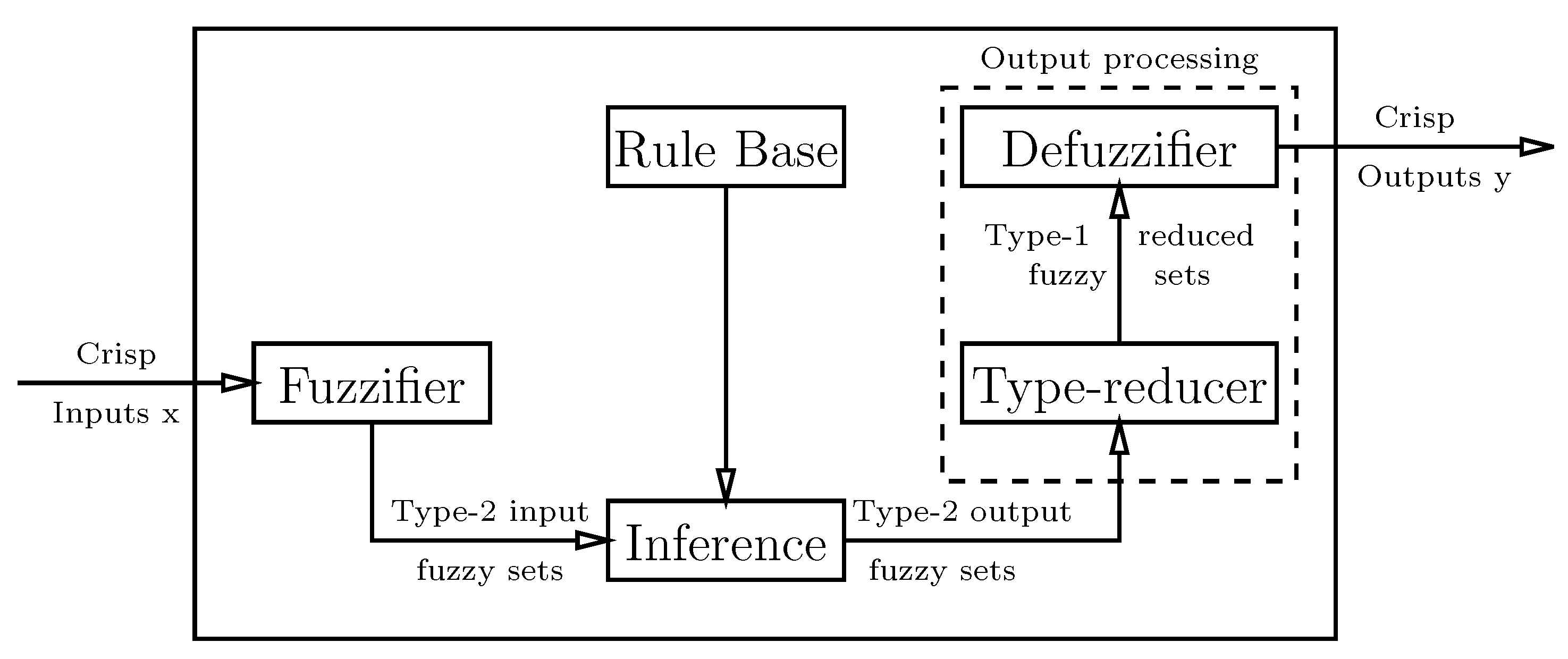
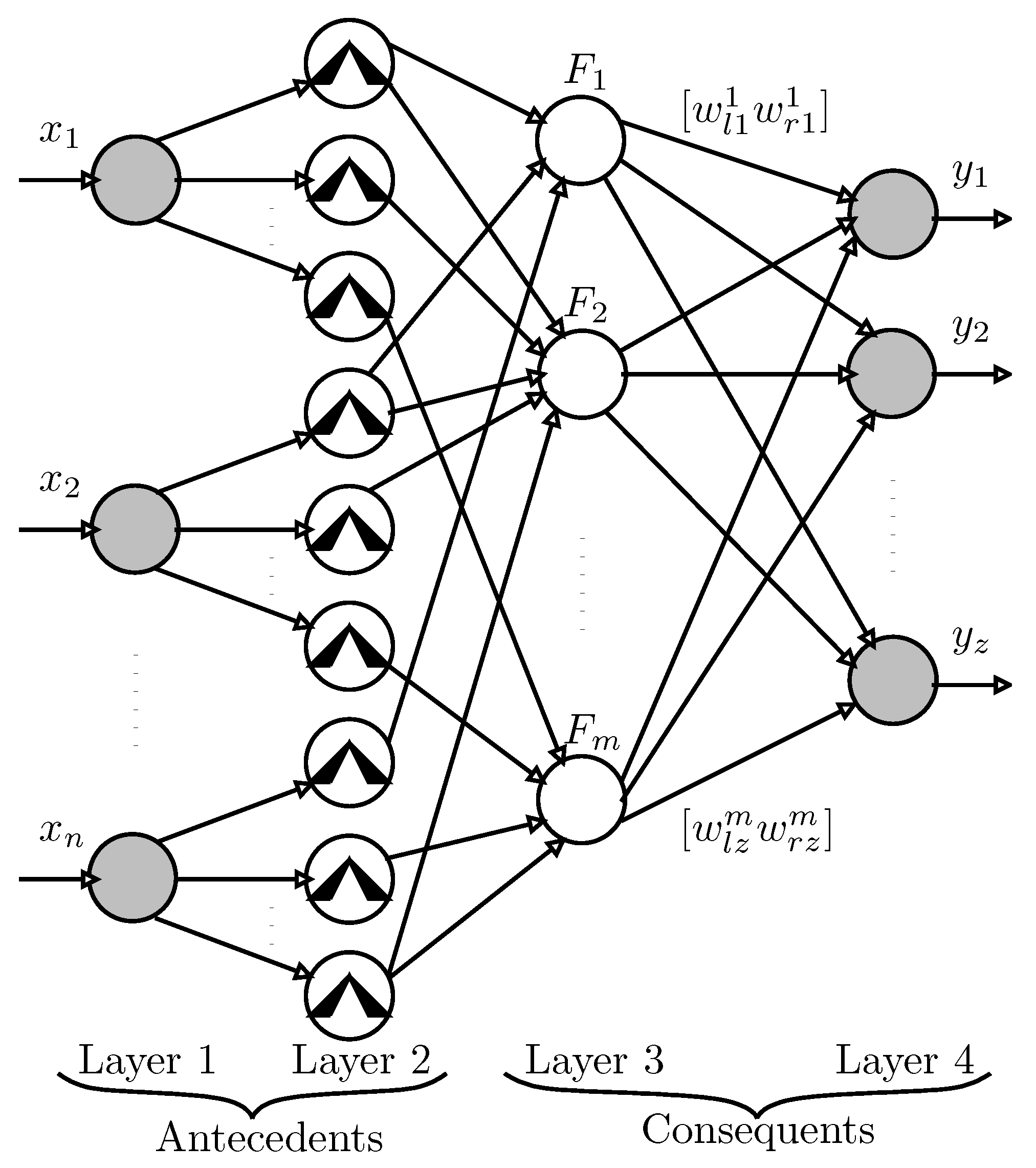
4. Interval Type-2 FLSs

The computation intensity of type-2 FLSs has been behind the development of interval fuzzy sets [56,57] as it provides a simplified and efficient way to compute meet and join operations and perform type-reduction for FLSs. It distributes the uncertainty evenly among all admissible primary memberships and offers a balanced trade-off between performance and complexity. Before proceeding further, a few concepts need to be introduced. An FLS with an interval singleton type-2 fuzzifier and product or minimum t-norm satisfies the following properties [57]:
  • the firing strength of the lth fuzzy rule is an interval type-1 fuzzy set defined as
    F l ( x ) i = 1 p μ F i l ˜ ( x i ) = [ f ̲ l ( x ) , f ¯ l ( x ) ] [ f ̲ l , f ¯ l ]
    where
    f ̲ l ( x ) = μ ̲ F 1 l ˜ ( x 1 ) μ ̲ F p l ˜ ( x p )
    f ¯ l ( x ) = μ ¯ F 1 l ˜ ( x 1 ) μ ¯ F p l ˜ ( x p )
    with the t-norm operator denoted by “⋆”.
  • the fired output consequent set of the lth rule is a type-1 fuzzy set characterized by a membership function
    μ B l ˜ ( y ) = b l [ f ̲ l μ ̲ G l ˜ ( y ) , f ¯ l μ ¯ G l ˜ ( y ) ] 1 / b l y Y
    with μ ̲ G l ˜ ( y ) and μ ¯ G l ˜ ( y ) being the lower and upper membership grades of μ G l ˜ ( y ) .
  • if N out of a total of L fuzzy rules in the FLS fire, where N L , then the overall aggregated output fuzzy set is defined by a type-1 membership function μ B ˜ ( y ) obtained by combining the fired output consequent sets into one. In other words, μ B ˜ ( y ) = l = 1 N μ B l ˜ ( y ) , where μ B l ˜ ( y ) is defined in Equation (5).
The following is a brief description of the different stages of the type-2 fuzzy logic inference engine.
μ B l ˜ ( y ) = b [ f ̲ 1 μ ̲ G 1 ˜ ( y ) ] [ f ̲ N μ ̲ G N ˜ ( y ) ] , [ f ¯ 1 μ ¯ G 1 ˜ ( y ) ] [ f ¯ N μ ¯ G N ˜ ( y ) ] 1 / b l , y Y

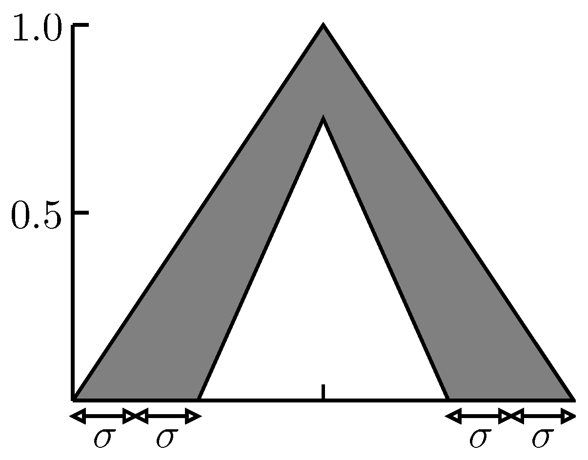
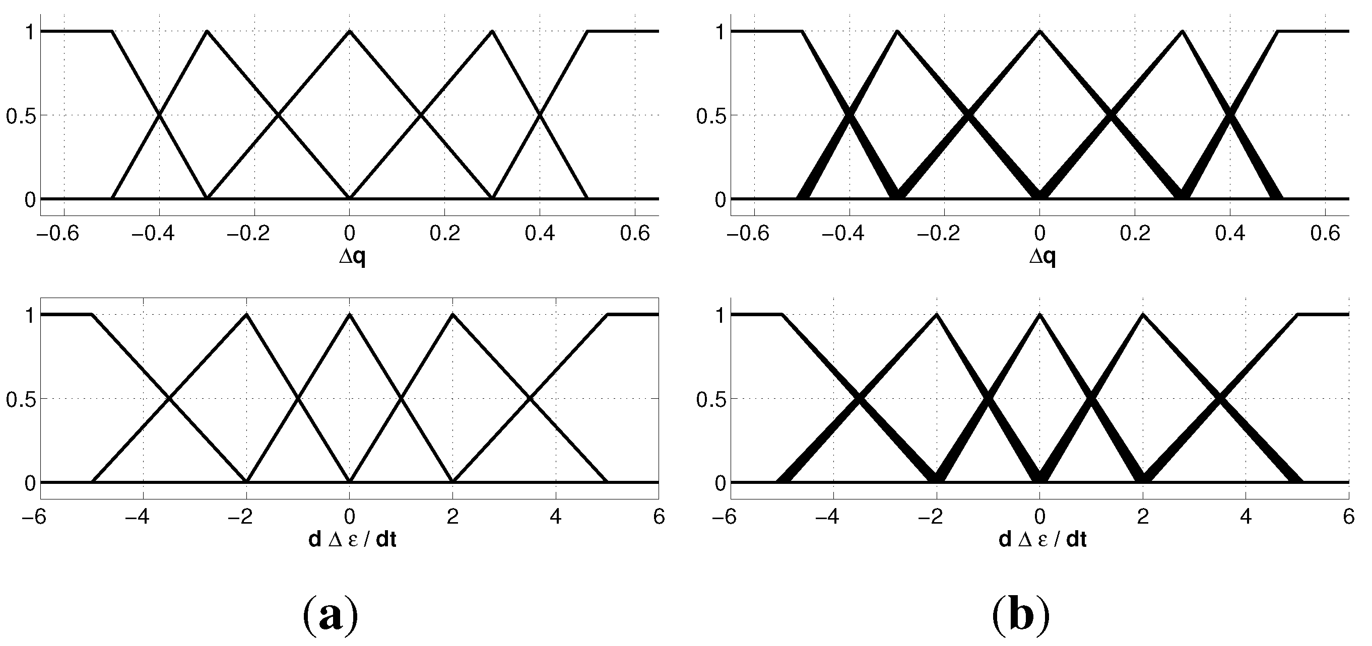
4.1. Type-2 Fuzzification

In the fuzzification stage, the crisp input vector with n elements x = ( x 1 , , x n ) T in the universe of discourse X 1 × X 2 × × X n is mapped into type-2 fuzzy sets [56,57]. The type-2 fuzzification process is schematically depicted in Figure 5. The upper and lower membership functions are computed for each point of the universe of discourse, resulting in an interval type-1 set [ f ̲ l , f ¯ l ] for each rule l.
Figure 5. Interval type-2 inference process.
Robotics 02 00066 g005

4.2. Type-2 Fuzzy Rule Base

Type-2 IF-THEN rules have the same structure as their type-1 counterpart. However, the antecedents and the consequents are represented by interval type-2 fuzzy sets. Thus, the l t h rule is of the form:
R l : IF  x 1  is  F ˜ 1 l  and  x 2  is  F ˜ 2 l  and and  x n  is  F ˜ n l
THEN  y 1  is  G ˜ 1 l  and  y 2  is  G ˜ 2 l  and and  y m  is  G ˜ m l
where ˜ is type-2 fuzzy set.

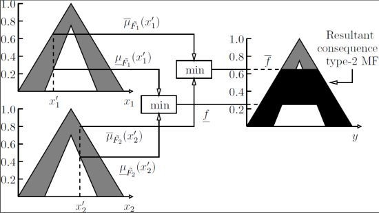
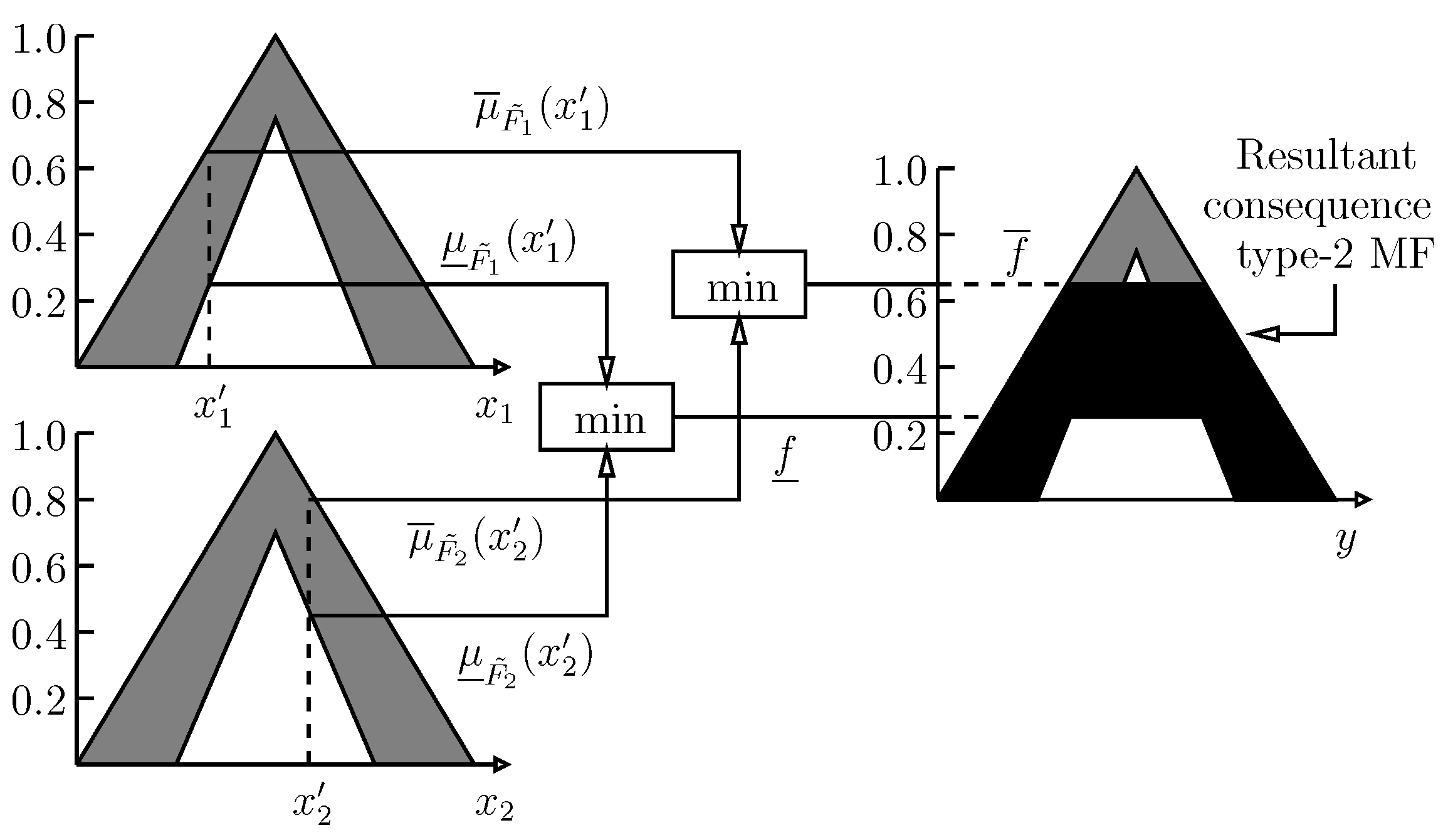
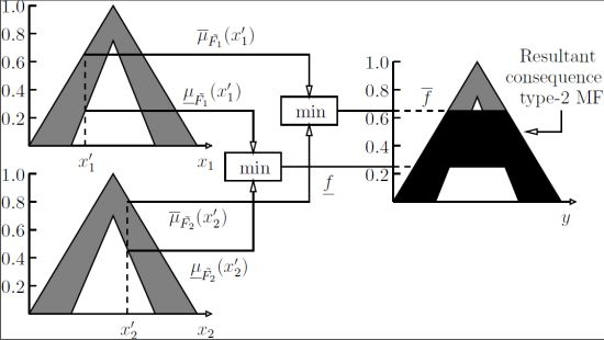
4.3. Type-2 Fuzzy Inference Engine

A type-2 fuzzy inference engine provides a mapping from the input type-2 fuzzy sets to the output ones. Each rule l in the knowledge base is interpreted as a type-2 fuzzy implication that, when aggregated with the fuzzified inputs, infers a type-2 fuzzy set B ˜ l such that:
μ B l ˜ ( y ) = x X [ μ A x ˜ ( x ) μ R l ( x , y ) ]
The t-norm and t-conorm used for the type-2 FLC herein are the “minimum” and “maximum” operators, respectively. These operators have been accredited in the literature for their computational efficiency and satisfactory performance.

4.4. Type Reduction

Type-reduction is an “extended version” of type-1 defuzzification methods (using the extension principle) because this operation reduces a type-2 output fuzzy set to a type-1 fuzzy set, which is called the “type-reduced set”. Several type-reduction methods have been suggested in the literature, such as the center-of-sums, the height, the modified height and the center-of-sets. The calculation of type-reduced sets is performed in two stages. First, the centroids of the type-2 interval consequent sets of the fuzzy rules are computed. This is conducted ahead of time and is not part of the control cycle. In the second stage, the type-reduced sets are computed at each control cycle before being defuzzified [54].
Calculation of the Rule Consequents Centroids The centroid of the t t h output fuzzy set y k t is a type-1 interval set determined by its left and right most points, y l k t and y r k t , respectively, which are expressed by [57]:
y k t = [ y l k t , y r k t ] = y ( θ 1 , , θ z ) = z = 1 Z y z θ z z = 1 Z θ z
Algorithm 1 describes the iterative procedures for computing y r k t and y l k t [54]. Without loss of generality, we assume that y z , z = 1 , , Z , are arranged in an ascending order; i.e., y 1 y 2 y Z .
Note that both algorithms are guaranteed to converge in at most Z iterations. However, as mentioned earlier, these procedures are conducted ahead of time and are not part of the control cycle. Such a property helps alleviate the heavy computational burden that is usually associated to computational intelligence-based controllers in general.

4.5. Calculation of the Type-Reduced Set

Using the centroid method, the center-of-sets type reduction reduces the resulting type-2 fuzzy sets to an interval type-1 fuzzy set [ y l k i , y r k i ] for each rule i. The inferred interval type-1 fuzzy set is then defined by [ y l k , y r k ] , such as:
y l k = i = 1 L f l i y l k i i = 1 L f l i
y r k = i = 1 L f r i y r k i i = 1 L f r i
where f l i , f r i are the firing strengths corresponding to y l k i and y r k i of rule i, to minimize y l k i and maximize y r k i . Algorithms 2 and 3 reveal the iterative procedures to compute y l k and y r k , respectively [57]. Without loss of generality, we here assume that the pre-computed y l k i , i = 1 , , L , are arranged in an ascending order; i.e., y l k 1 y l k 2 y l k L . Hence, y l k and y r k can be mathematically expressed as:
y l k = u = 1 Q f ¯ u y l k u + v = Q + 1 L f ̲ v y l k v u = 1 Q f ¯ u + v = Q + 1 L f ̲ v y r k = u = 1 R f ̲ u y r k u + v = R + 1 L f ¯ v y r k v u = 1 R f ̲ u + v = R + 1 L f ¯ v
It is worth pointing out that both procedures are proven to converge in no more than L iterations, where L is the total number of rules [57].
Robotics 02 00066 i001
Robotics 02 00066 i002
Robotics 02 00066 i003

4.6. Type-2 Defuzzification

The type-reduced set Y c o s ( X ) k determined by its left most and right most points, y l k and y r k , respectively, is defuzzified using the interval set average formula to get a crisp output value. As such, the defuzzified crisp output for each output k is formulated as [56]:
Y k ( x ) = y l k + y r k 2
In this work, we are concerned with adaptive type-2 FLC, and hence, Algorithms 1–3 will be replaced with the adaptive mechanism explained in the next section. As such, we overcome the heavy computational burden traditionally associated to computational intelligence-based controllers.

5. Control Strategy

Let Δ q = q d q and Δ θ = θ d θ denote the links’ and actuators’ position errors, respectively, with θ d being the unknown desired time-dependent motor position vector. The control strategy is based on the design of an adaptive controller that not only leads to a precise tracking of the system’s nominal desired signals but also improves the motors’ internal stability. Should the motors’ desired position θ d have been available, the control strategy would be based on tracking Δ q and Δ θ to zero. Since that is not the case, we define the following compounded velocity error signal:
Δ ϵ ˙ r = q ˙ d λ q ˙ + ( 1 λ ) 1 r θ ˙
for a diagonal matrix λ = diag ( λ 1 , λ 2 , , λ n ) with λ i [ 0 , 1 ] , i = 1 , , n . The feedback gain λ is introduced to provide a trade-off between the link tracking performance and internal stability, due to the high nonlinear coupling between the two. Note how a choice of λ i = 1 , i { 1 , , n } , completely annihilates the motor’s internal stability factor. The fuzzy control strategy is based on a human operator experience to interpret a situation and initiate its control action. A block diagram for the fuzzy controller is illustrated in Figure 6. Given the desired control signals q d and q ˙ d , the link’s position error Δ q and the compounded velocity error Δ ϵ ˙ r are computed. The FLC takes these two inputs and provides a control action τ m that is proportional to the input values. These signals are quantized into 5 levels represented by a set of linguistic variables: Negative Large (NL), Negative Small (NS), Zero (Z), Positive Small (PS), and Positive Large (PL). In this study, triangular membership functions are used, mainly due to their high computational and performance efficiencies [58]. To assess the performance of both types of controllers, the proposed fuzzy controller is implemented in two different ways: the first is based on a type-1 fuzzy control scheme while the second is based on a type-2. The input membership functions adopted by both types of control systems are shown in Figure 7. In order to perform a fair comparison between type-1 and type-2 FLCs, the type-2 membership functions have been designed such that they are very similar to those of type-1 and have small blurbs in their FOUs. The fuzzy rules of the two control techniques are the same, they were chosen heuristically and can be refined by an expert (see Table 1). These rules are based on three hypotheses: (i) when the input signals are far from their respective nominal zero-valued surfaces, then the FLC’s output assumes a high value; (ii) when the inputs are approaching the nominal zero-valued surfaces, the output is adjusted to a smaller value for a smoother approach; (iii) once the inputs are on the nominal zero-valued surfaces, then the output is set to zero. This way, the FLC forces the link position error Δ q and the compounded velocity error Δ ϵ ˙ r to approach zero. It is worth mentioning that an empirical study was conducted beforehand to tune the input membership functions. The center of area method is used for defuzzification.
Figure 6. Block diagram of the proposed fuzzy control scheme.
Robotics 02 00066 g006
Figure 7. Fuzzy membership functions: (a) type-1; and (b) type-2.
Robotics 02 00066 g007
Table 1. Fuzzy rules for type-1 and type-2 FLCs.
Δ q
Δ ϵ ˙ r NLNSZPSPL
PLZPLPLPLPL
PSNSZPSPSPL
ZNLNSZPSPL
NSNLNSNSZPS
NLNLNLNLNLZ

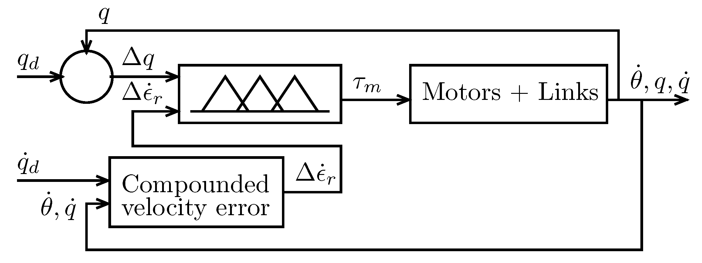
5.1. Adaptive Type-2 FLC

The adaptive type-2 FLC structure is depicted in Figure 8. It consists of four layers. Input nodes and type-2 fuzzification nodes are shown in layer 1 and layer 2, respectively, forming the antecedent part of the fuzzy rules. Consequent parts are represented by layers 3 and 4, which are constructed with fuzzy rule nodes and output nodes. They are linked by interval weighting factors [ w l z m w r z m ] .
The adaptive type-2 FLC’s output can be written as:
Y = Φ T w + ϵ = Φ T w ^
where w R z × m is a weight matrix and Φ is a m-dimensional vector of known functions (regressor).
Figure 8. Adaptive Type-2 fuzzy logic control structure.
Robotics 02 00066 g008
Define the following signals:
s = Δ ϵ ˙ r + Ψ Δ q = q r ˙ Λ q ˙ ( 1 Λ ) 1 r θ ˙
q r ˙ = q d ˙ + Ψ Δ q
where Ψ = [ ψ 1 , ψ 2 , , ψ n ] with ψ i being a positive constant, i = 1 , , n .
Recall Euler–Lagrange formulation (1):
M ( q ) q ¨ + C ( q , q ˙ ) q ˙ + G ( q ) + τ f l + τ d l τ t = 0
J m θ ¨ + τ f m + τ d m τ m = 1 r τ t
where q, q ˙ , q ¨ , θ ¨ R n . Substituting for τ t , and letting the stiffness constant K tend to infinity (singular perturbation), we obtain the following rigid model [16]:
M t ( q ) q ¨ + C ( q , q ˙ ) q ˙ + G ( q ) + τ F r d = τ m
where,
M t ( q ) = J m r + M ( q ) τ F r d = τ f l + τ d l + τ f m r + τ d m r + ( 1 r ) τ m
Using the linear in parameters property of the manipulator dynamics, we can approximate the model with a linear regression:
M t ( q ) q ¨ r + C ( q , q ˙ ) q ˙ r + G ( q ) + τ F r d = Φ ( q ¨ r , q ˙ r , q ˙ , q ) T w
The control law is:
τ m = Φ T w ^ + K D s
where K D is a positive diagonal matrix gain and the sign ^ denotes the parameter estimate vector.
Theorem 1 
Consider the nonlinear system in Equation (1) with reference signal (11) and control law (14). The adaptive control law is asymptotically stable and the tracking error converges to zero with the following adaptation law:
w ^ ˙ = Γ Φ s
where Γ = d i a g ( γ 1 , γ 2 , , γ n ) and γ i is a positive constant, i = 1 , , n .
Proof: 
Taking the derivative of the error signal s yields
s ˙ = q ¨ r Λ q ¨ ( 1 Λ ) 1 r θ ¨
Let K , i.e., displacement ( θ q ) 0 . We get:
s ˙ = q ¨ r q ¨
M t ( q ) s ˙ = M t ( q ) q ¨ r M t ( q ) q ¨
Substituting M q ¨ from Equation (13):
M t ( q ) s ˙ = M t ( q ) q ¨ r + C ( q , q ˙ ) q ˙ r + G ( q ) + τ F r d C ( q , q ˙ ) s τ m
The linear in parameters property yields
M t ( q ) s ˙ = Φ T w C ( q , q ˙ ) s τ m
Set
τ m = Φ T w ^ + K D s
Equation (15) becomes
M t ( q ) s ˙ = Φ T w ˜ C ( q , q ˙ ) s K D s
where w ˜ = w w ^ .
Choose the following Lyapunov candidate:
V = 1 2 { s T M t ( q ) s + w ˜ T Γ 1 w ˜ }
Taking the derivative of V:
V ˙ = s T M t ( q ) s ˙ + 1 2 s T M ˙ t ( q ) s + w ˜ T Γ 1 w ^ ˙
Substituting for M t ( q ) s ˙ :
V ˙ = s T Φ T w ˜ + s T { 1 2 ( M ˙ t ( q ) 2 C ( q , q ˙ ) ) } s + w ˜ T Γ 1 w ^ ˙ s T K D s
s T { ( M ˙ t ( q ) 2 C ( q , q ˙ ) ) } s = 0 due to the skew-symmetry property. Hence,
V ˙ = s T Φ T w ˜ + w ˜ T Γ 1 w ^ ˙ s T K D s
Setting the adaptation law as
w ^ ˙ = Γ Φ s
leads to
V ˙ = s T K D s 0
Therefore V, and so s, w ˜ and w ^ , are bounded and converge to finite values. It follows from Equation (16) that τ m is bounded, which implies that all the terms in Equation (17), including s ˙ , are bounded. Thus, V ¨ = 2 s T K D s ˙ is also bounded. Hence, from Barbalet’s Lemma, it implies that lim t V ˙ = 0 . Therefore, lim t s = 0 .

6. Simulation Results and Discussion

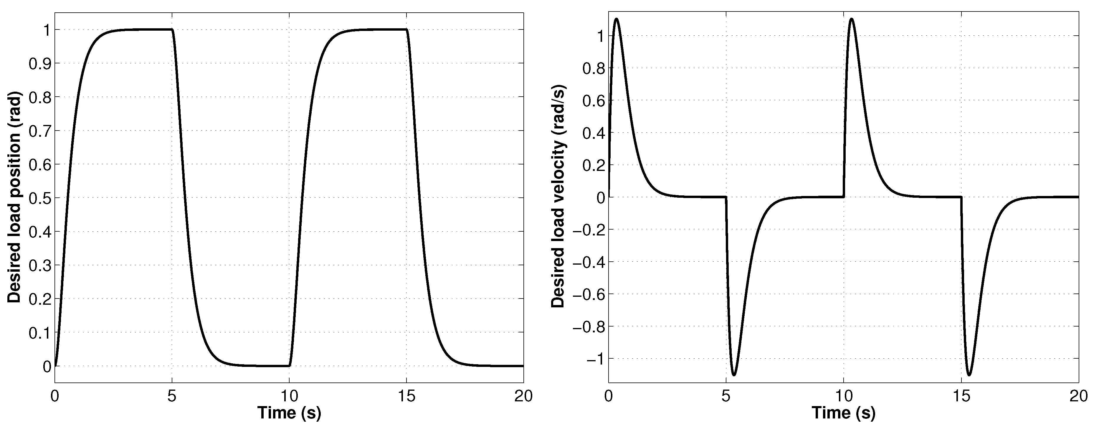
6.1. Simulation Setup

To demonstrate the performance of the proposed controller, two numerical simulations are carried out on a single link flexible-joint manipulator. Table 2 summarizes the manipulator’s physical parameters along with their respective values. The stiffness coefficient and gear ratio are set to be K = 7 N·m/rad and r = 1 , respectively. The link’s mass and length are taken as m = 0 . 21 Kg and l = 0 . 3 m, respectively. The manipulator’s dynamics in terms of its physical parameters is defined by: M ( q ) = I , C ( q , q ˙ ) = 0 , and G ( q ) = m g l sin ( q ) , where g = 9 . 8 m/s 2 is the gravitational constant and I is the link’s rotational inertia given in Table 2. The nonlinear friction model described in Section 2 is considered to model the actuator’s and load’s mechanical frictions, τ f m and τ f l , respectively.
Table 2. Manipulators physical parameters.
ParameterLinkMotor
rotational inertia (kg·m 2 ) I = 5.05 × 10 2 J m = 4 × 10 3
viscous friction coefficient (N·m·s/rad) F v l = 4 × 10 3 F v m = 3 × 10 3
Coulomb friction coefficient (N·m) F c l = 1 × 10 2 F c m = 4 × 10 3
static friction coefficient (N·m) F s l = 2 × 10 3 F s m = 2 × 10 3
static friction decreasing rate (rad/s) η s l = 7 × 10 2 η s m = 5 × 10 2
The manipulator’s desired position trajectory is taken as the step response of a critically damped second order system with a natural frequency of 3 rad/s, as shown in Figure 9. The feedback gain λ in Equation (9) is set to 0.8. The control structure scheme and the system’s model are implemented in Simulink TM while the fuzzy control engines are programmed in C. Both controllers are set to operate at a bandwidth of 100 Hz.
Figure 9. Manipulator’s position and velocity reference signals.
Robotics 02 00066 g009

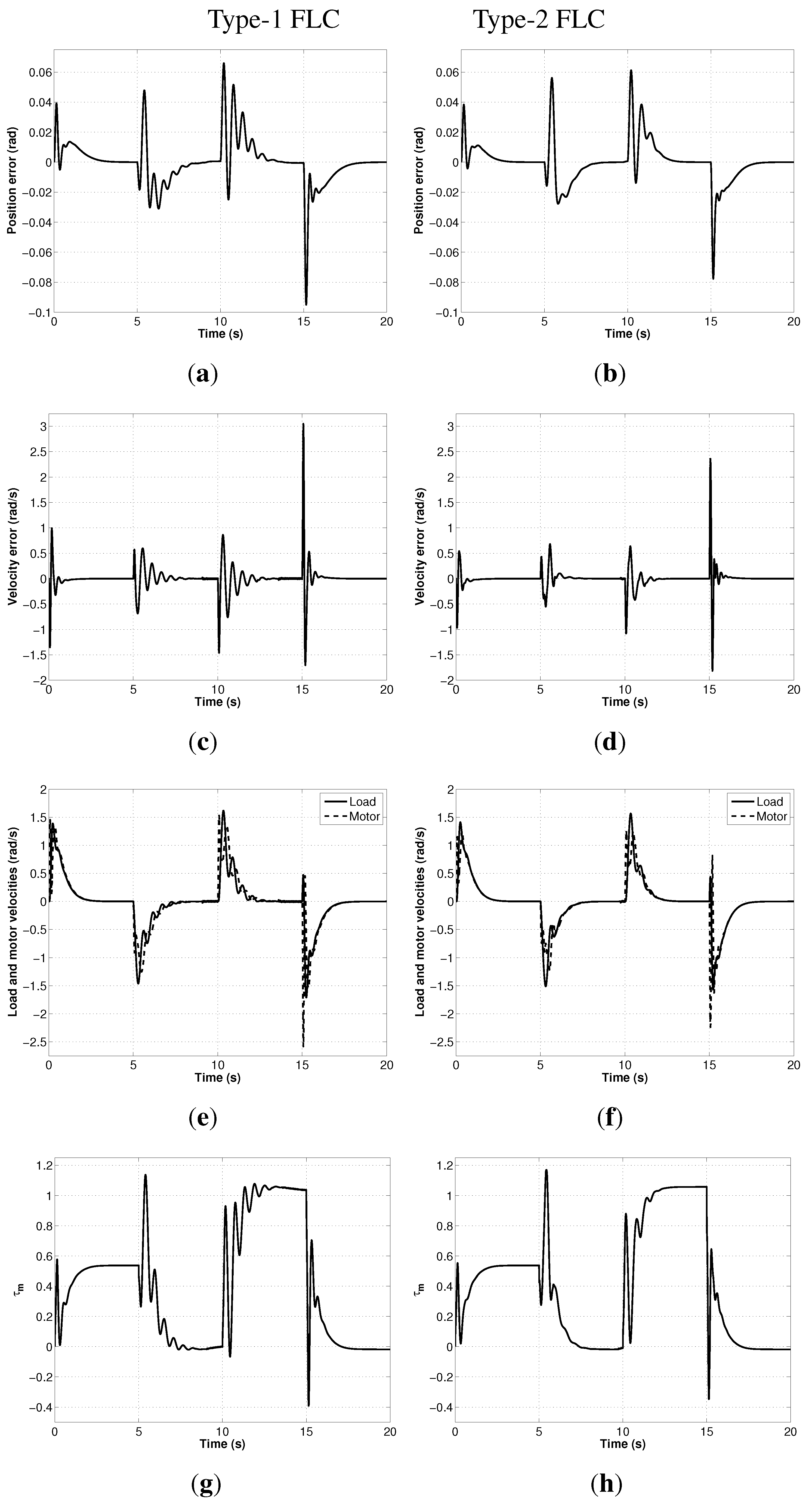
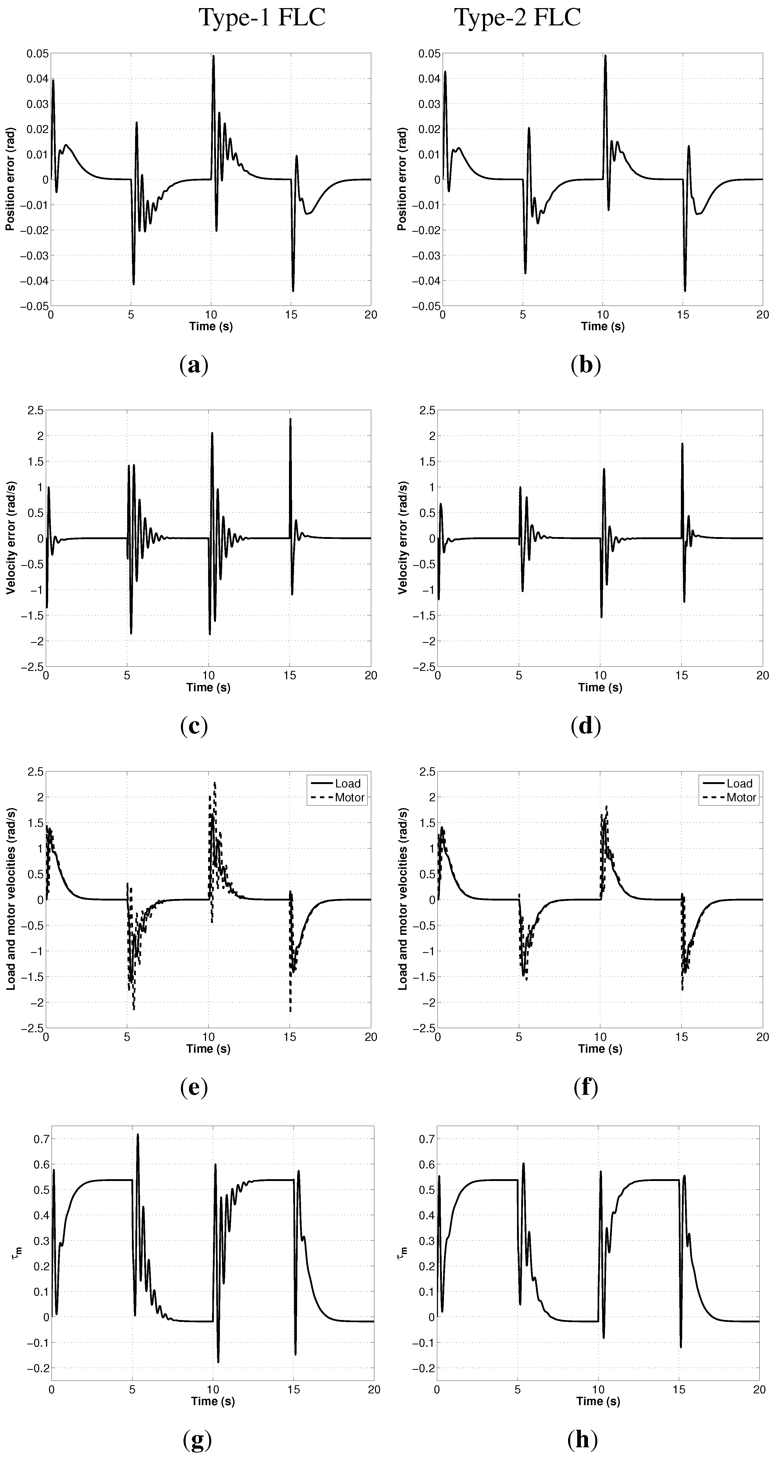
6.2. Numerical Simulations and Results

Two simulations are carried out to highlight the proposed type-2 FLC as opposed to type-1 in tolerating a higher degree of parametric and modeling uncertainties. In both simulations, the system’s dynamics is assumed to be a priori unknown. For each simulation, the system’s response is studied taking into account the manipulator’s position and velocity errors, the joint’s internal stability, and the controller’s output torque, τ m .
The first simulation is meant to study the controller’s ability to sustain various types and magnitudes of load uncertainties. For this purpose, the load’s inertia and the link’s mass are both doubled abruptly at 5 s and returned back to their original values at 15 s of the simulation. The results are shown in Figure 10. A slight increase is noticed in the manipulator’s position and velocity errors due to a heavier load. However, the error signals and the controller’s output under type-1 FLC are fairly fluctuating as opposed to a smooth and steady convergence behavior with the type-2 FLC. It is quite important to notice here the degradation in the actuator’s internal stability (Figure 10(e)) under type-1 FLC despite the settling of the load’s velocity. The superiority of the adaptive type-2 FLC in compensating for such a type of uncertainty is manifested with a better load position, speed accuracy and control effort performance over its type-1 counterpart.
In the second simulation, the elastic joint’s stiffness coefficient is changed abruptly to K = 5 N·m/rad at 5 s and returned back to its original value ( K = 7 N·m/rad) at 15 s of the simulation. The controller’s performance under such conditions is revealed in Figure 11. As in simulation 1, adaptive type-1 FLC is able to maintain bounded error signals but fails to make them converge smoothly. This is especially clear with the load’s position and velocity errors (Figure 11(a) and Figure 11(c)) and the motor’s internal stability (Figure 11(e)). On the other hand, it is clear that the adaptive type-2 FLC does indeed maintain these signals smoother and with less control effort than its type-1 counterpart.
Figure 10. System’s response to varying load’s mass and inertia: (a), (b) manipulator’s position error; (c), (d) manipulator’s velocity error; (e), (f) motor’s velocity vs. manipulator’s velocity; and (g), (h) controller’s output torque ( τ m ).
Robotics 02 00066 g010
Figure 11. System’s response to varying stiffness coefficient: (a), (b) manipulator’s position error; (c), (d) manipulator’s velocity error; (e), (f) motor’s velocity vs. manipulator’s velocity; and (g), (h) controller’s output torque ( τ m ).
Robotics 02 00066 g011

7. Conclusions

In this paper, an adaptive type-2 FLC with a Mamdani inference engine has been proposed for flexible-joint manipulators in the presence of dynamical modeling and parametric uncertainties of various magnitudes. The control strategy takes into account the actuators’ relative stability by introducing a trade-off criterion between the actuators’ internal stability and the links’ position. A comparison of the proposed controller and its type-1 counterpart is performed under similar operating conditions. The simulations show the superiority of the adaptive type-2 FLC in compensating for high magnitude of uncertainties, which confirms the theoretical credentials associated to type-2 FLSs.

Acknowledgements

The authors would like to acknowledge Natural Sciences and Engineering Research Council of Canada (NSERC) for partially supporting this work through the Discovery program.

Conflict of Interest

The authors declare no conflict of interest.

References

  1. Olsson, H.; Astrom, K.; de Wit, C.C.; Gafvert, M.; Lischinsky, P. Friction models and friction compensation. Eur. J. Control 1998, 4, 176–195. [Google Scholar]
  2. Seidl, D.R.; Lam, S.L.; Putman, J.A.; Lorenz, R.D. Neural network compensation of gear backlash hysteresis in position-controlled mechanisms. IEEE Trans. Ind. Appl. 1995, 31, 1475–1483. [Google Scholar] [CrossRef]
  3. Sweet, L.; Good, M. Redefinition of the robot motion-control problem. Control Syst. Mag. IEEE 1985, 5, 18–25. [Google Scholar] [CrossRef]
  4. Armstrong, B.; de Wit, C.C. Friction modeling and compensation. Control Handb. 1996, 77, 1369–1382. [Google Scholar]
  5. Ghorbel, F.; Hung, J.; Spong, M. Adaptive control of flexible-joint manipulators. Control Syst. Mag. IEEE 1989, 9, 9–13. [Google Scholar] [CrossRef]
  6. Seidl, D.; Lam, S.L.; Putman, J.; Lorenz, R. Neural network compensation of gear backlash hysteresis in position-controlled mechanisms. IEEE Trans. Ind. Appl. 1995, 31, 1475–1483. [Google Scholar] [CrossRef]
  7. Seidl, D.; Reineking, T.; Lorenz, R. Neural Network Compensation of Gear Backlash Hysteresis in Position-Controlled Mechanisms. In Proceedings of Conference Record of the IEEE Industry Applications Society Annual Meeting, Houston, TX, USA, October 1992; Volume 2, pp. 1937–1944.
  8. Benosman, M.; Vey, G.L. Control of flexible manipulators: A survey. Robotica 2004, 22, 533–545. [Google Scholar] [CrossRef]
  9. Chaoui, H.; Gueaieb, W. Type-2 fuzzy logic control of a flexible-joint manipulator. J. Intell. Robot. Syst. 2008, 51, 159–186. [Google Scholar] [CrossRef]
  10. Chaoui, H.; Sicard, P.; Gueaieb, W. ANN-based adaptive control of robotic manipulators with friction and joint elasticity. IEEE Trans. Ind. Electron. 2009, 56, 3174–3187. [Google Scholar] [CrossRef]
  11. Luca, A.D.; Isidori, A.; Nicolo, F. Control of Robot Arm with Elastic Joints via Nonlinear Dynamic Feedback. In Proceedings of the IEEE Conference on Decision and Control Including the Symposium on Adaptive Processes, Ft. Lauderdale, FL, USA, 11–13 December 1985; pp. 1671–1679.
  12. Khorasani, K. Nonlinear feedback control of flexible joint manipulators: A single link case study. IEEE Trans. Autom. Control 1990, 35, 1145–1149. [Google Scholar] [CrossRef]
  13. De Wit, C. Robust control for servo-mechanisms under inexact friction compensation. Automatica 1993, 29, 757–761. [Google Scholar] [CrossRef]
  14. Ott, C.; Albu-Schaffer, A.; Hirzinger, G. Comparison of Adaptive and Nonadaptive Tracking Control Laws for a Flexible Joint Manipulator. In Proceedings of the IEEE International Conference on Intelligent Robots and Systems, Lausanne, Switzerland, 30 September–4 October 2002; Volume 2, pp. 2018–2024.
  15. Al-Ashoor, R.; Patel, R.; Khorasani, K. Robust adaptive controller design and stability analysis for flexible-joint manipulators. IEEE Trans. Syst. Man Cybern. 1993, 23, 589–602. [Google Scholar] [CrossRef]
  16. Ghorbel, F.; Spong, M.W. Adaptive Integral Manifold Control of Flexible Joint Robot Manipulators. In Proceedings of the IEEE International Conference on Robotics and Automation, Nice, France, 12–14 May 1992; Volume 1, pp. 707–714.
  17. Spong, M.W. Modeling AND control of elastic joint robots. J. Dyn. Syst. Meas. Control 1987, 109, 310–319. [Google Scholar] [CrossRef]
  18. Ge, S.S.; Postlethwaite, I. Adaptive neural network controller design for flexible joint robots using singular perturbation technique. Trans. Inst. Meas. Control 1995, 17, 120–131. [Google Scholar]
  19. Taghirad, H.; Khosravi, M. Design and Simulation of Robust Composite Controllers for Flexible Joint Robots. In Proceedings of the IEEE International Conference on Robotics and Automation, Taipei, Taiwan, 14–19 September 2003; Volume 3, pp. 3108–3113.
  20. Huang, L.; Ge, S.; Lee, T. Adaptive Position/force Control of an Uncertain Constrained Flexible Joint Robots-Singular Perturbation Approach. In Proceedings of the SICE Annual Conference, Sapporo, Japan, 4–6 August 2004; pp. 1693–1698.
  21. Spong, M. Modeling and control of elastic joint robots. J. Dyn. Syst. Meas. Control 1987, 109, 310–319. [Google Scholar] [CrossRef]
  22. Khorasani, K. Adaptive control of flexible joint robots. IEEE Trans. Robot. Autom. 1992, 8, 250–267. [Google Scholar] [CrossRef]
  23. Ott, C.; Albu-Schaffer, A.; Kugi, A.; Stramigioli, S.; Hirzinger, G. A Passivity Based Cartesian Impedance Controller for Flexible Joint Robots-Part I: Torque Feedback and Gravity Compensation. In Proceedings of the IEEE International Conference on Robotics and Automation, New Orleans, LA, USA, 26 April–1 May 2004; pp. 2659–2665.
  24. Tian, L.; Goldenberg, A. Robust Adaptive Control of Flexible Joint Robots with Joint Torque Feedback. In Proceedings of the IEEE International Conference on Robotics and Automation, Nagoya, Japan, May 1995; Volume 1, pp. 1229–1234.
  25. Sun, T.; Pei, H.; Pan, Y.; Zhou, H.; Zhang, C. Neural network-based sliding mode adaptive control for robot manipulators. Neurocomputing 2011, 74, 2377–2384. [Google Scholar] [CrossRef]
  26. Li, Y.; Tong, S.; Li, T. Adaptive fuzzy output feedback control for a single-link flexible robot manipulator driven DC motor via backstepping. Nonlinear Anal. R. World Appl. 2013, 14, 483–494. [Google Scholar] [CrossRef]
  27. Yen, H.M.; Li, T.H.S.; Chang, Y.C. Adaptive neural network based tracking control for electrically driven flexible-joint robots without velocity measurements. Comput. Math. Appl. 2012, 64, 1022–1032. [Google Scholar] [CrossRef]
  28. Lopez-Araujo, D.J.; Zavala-Rio, A.; Santibanez, V.; Reyes, F. Output-feedback adaptive control for the global regulation of robot manipulators with bounded inputs. Int. J. Control Autom. Syst. 2013, 11, 816–822. [Google Scholar] [CrossRef]
  29. Fateh, M.M. Nonlinear control of electrical flexible-joint robots. Nonlinear Dyn. 2011, 67, 2549–2559. [Google Scholar] [CrossRef]
  30. Fateh, M.M.; Khorashadizadeh, S. Robust control of electrically driven robots by adaptive fuzzy estimation of uncertainty. Nonlinear Dyn. 2012, 69, 1465–1477. [Google Scholar] [CrossRef]
  31. Islam, S.; Liu, P.X. Robust sliding mode control for robot manipulators. IEEE Trans. Ind. Electron. 2011, 58, 2444–2453. [Google Scholar] [CrossRef]
  32. Corradini, M.L.; Fossi, V.; Giantomassi, A.; Ippoliti, G.; Longhi, S.; Orlando, G. Discrete time sliding mode control of robotic manipulators: Development and experimental validation. Control Eng. Pract. 2012, 20, 816–822. [Google Scholar] [CrossRef]
  33. Islam, S.; Liu, P.X. Robust adaptive fuzzy output feedback control system for robot manipulators. ASME/IEEE Trans. Mechatron. 2011, 16, 288–296. [Google Scholar] [CrossRef]
  34. Karray, F.; Gueaieb, W.; Al-Sharhan, S. The hierarchical expert tuning of PID controllers using tools of soft computing. IEEE Trans. Syst. Man Cybern. 2002, 32, 77–90. [Google Scholar] [CrossRef] [PubMed]
  35. De Silva, C.W. Intelligent Control Fuzzy Logic Applications; CRC Press: Boca Raton, FL, USA, 1995. [Google Scholar]
  36. Kim, E. Output feedback tracking control of robot manipulators with model uncertainty via adaptive fuzzy logic. IEEE Trans. Fuzzy Syst. 2004, 12, 368–378. [Google Scholar] [CrossRef]
  37. Gueaieb, W.; Karray, F.; Al-Sharhan, S. A robust adaptive fuzzy position/force control scheme for cooperative manipulators. IEEE Trans. Control Syst. Technol. 2003, 11, 516–528. [Google Scholar] [CrossRef]
  38. Chaoui, H.; Sicard, P.; Lakhsasi, A.; Schwartz, H. Neural Network Based Model Reference Adaptive Control Structure for a Flexible Joint with Hard Nonlinearities. In Proceedings of the IEEE International Symposium on Industrial Electronics, Ajaccio, France, 4–7 May 2004; Volume 1, pp. 271–276.
  39. Chaoui, H.; Sicard, P.; Lakhsasi, A. Reference Model Supervisory Loop for Neural Network Based Adaptive Control of a Flexible Joint with Hard Nonlinearities. In Proceedings of the IEEE Canadian Conference on Electrical and Computer Engineering, Niagara Falls, ON, Canada, 2–5 May 2004; Volume 4, pp. 2029–2034.
  40. Chaoui, H.; Gueaieb, W.; Yagoub, M.; Sicard, P. Hybrid Neural Fuzzy Sliding Mode Control of Flexible-Joint Manipulators with Unknown Dynamics. In Proceedings of the 32nd Annual Conference of the IEEE Industrial Electronics Society (IECON-2006), Paris, France, 6–10 November 2006; pp. 4082–4087.
  41. Chaoui, H.; Gueaieb, W.; Yagoub, M.C. Artificial Neural Network Control of a Flexible-Joint Manipulator under Unstructured Dynamic Uncertainties. In Proceedings of the IEEE International Workshop on Robotic and Sensors Environments, Ottawa, ON, Canada, 12–13 October 2007.
  42. Hui, D.; Fuchun, S.; Zengqi, S. Observer-based adaptive controller design of flexible manipulators using time-delay neuro-fuzzy networks. J. Intell. Robot. Syst. Theory Appl. 2002, 34, 453–466. [Google Scholar] [CrossRef]
  43. Subudhi, B.; Morris, A. Singular perturbation based neuro-H infinity control scheme for a manipulator with flexible links and joints. Robotica 2006, 24, 151–161. [Google Scholar] [CrossRef]
  44. Park, C.W. Robust stable fuzzy control via fuzzy modeling and feedback linearization with its applications to controlling uncertain single-link flexible joint manipulators. J. Intell. Robot. Syst. Theory Appl. 2004, 39, 131–147. [Google Scholar] [CrossRef]
  45. Li, T.H.S.; Huang, Y.C. MIMO adaptive fuzzy terminal sliding-mode controller for robotic manipulators. Inform. Sci. 2011, 180, 4641–4660. [Google Scholar] [CrossRef]
  46. Cazarez-Castro, N.R.; Aguilar, L.T.; Castillo, O. Designing type-1 and type-2 fuzzy logic controllers via fuzzy lyapunov synthesis for nonsmooth mechanical systems. Eng. Appl. Artif. Intell. 2012, 25, 971–979. [Google Scholar] [CrossRef]
  47. Castillo, O.; Melin, P. Optimization of type-2 fuzzy systems based on bio-inspired methods: A concise review. Inform. Sci. 2012, 205, 1–19. [Google Scholar] [CrossRef]
  48. Castillo, O.; Martinez-Marroquin, R.; Melin, P.; Valdez, F.; Soria, J. Comparative study of bio-inspired algorithms applied to the optimization of type-1 and type-2 fuzzy controllers for an autonomous mobile robot. Eng. Appl. Artif. Intell. 2012, 192, 19–38. [Google Scholar] [CrossRef]
  49. Melin, P.; Astudillo, L.; Castillo, O.; Valdez, F.; Garcia, M. Optimal design of type-2 and type-1 fuzzy tracking controllers for autonomous mobile robots under perturbed torques using a new chemical optimization paradigm. Expert Syst. Appl. 2013, 40, 3185–3195. [Google Scholar] [CrossRef]
  50. Feng, G. A survey on analysis and design of model-based fuzzy control systems. IEEE Trans. Fuzzy Sets Syst. 2006, 14, 676–697. [Google Scholar] [CrossRef]
  51. Chen, C.S. Supervisory adaptive tracking control of robot manipulators using interval type-2 TSK fuzzy logic system. IET Control Theory Appl. 2011, 5, 1796–1807. [Google Scholar] [CrossRef]
  52. Linda, O.; Manic, M. Uncertainty-robust design of interval type-2 fuzzy logic controller for delta parallel robot. IEEE Trans. Ind. Inf. 2011, 57, 661–670. [Google Scholar] [CrossRef]
  53. Biglarbegian, M.; Melek, W.W.; Mendel, J.M. Design of novel interval type-2 fuzzy controllers for modular and reconfigurable robots: Theory and experiments. IEEE Trans. Ind. Electron. 2011, 58, 1371–1384. [Google Scholar] [CrossRef]
  54. Hagras, H.A. A hierarchical type-2 fuzzy logic control architecture for autonomous mobile robots. IEEE Trans. Fuzzy Syst. 2004, 12, 524–539. [Google Scholar] [CrossRef]
  55. Sicard, P. Trajectory Tracking of Flexible Joint Manipulators with Passivity Based Controller. Ph.D. Thesis, Rensselaer Polytechnic Institute, Troy, NY, USA, 1993. [Google Scholar]
  56. Liang, Q.; Mendel, J.M. Interval type-2 fuzzy logic systems: Theory and design. IEEE Trans. Fuzzy Syst. 2000, 8, 535–550. [Google Scholar] [CrossRef]
  57. Mendel, J.M. Uncertain Rule-Based Fuzzy Logic Systems: Introduction and New Directions; Prentice-Hall: Upper Saddle River, NJ, USA, 2001. [Google Scholar]
  58. Pedryez, W. Why triangular membership functions? Fuzzy Sets Syst. 1994, 64, 21–30. [Google Scholar] [CrossRef]

