Article

IMU and Multiple RGB-D Camera Fusion for Assisting Indoor Stop-and-Go 3D Terrestrial Laser Scanning

1
Department of Geomatics Engineering, Schulich School of Engineering, University of Calgary, 2500 University Drive N.W., Calgary, AB T2N 1N4, Canada
2
Xsens Technologies B.V., Pantheon 6a, Enschede 7521 PR, The Netherlands
*
Author to whom correspondence should be addressed.
Robotics 2014, 3(3), 247-280; https://doi.org/10.3390/robotics3030247
Submission received: 19 February 2014 / Revised: 24 April 2014 / Accepted: 17 June 2014 / Published: 11 July 2014
(This article belongs to the Special Issue Robot Vision)

Abstract

:
Autonomous Simultaneous Localization and Mapping (SLAM) is an important topic in many engineering fields. Since stop-and-go systems are typically slow and full-kinematic systems may lack accuracy and integrity, this paper presents a novel hybrid “continuous stop-and-go” mobile mapping system called Scannect. A 3D terrestrial LiDAR system is integrated with a MEMS IMU and two Microsoft Kinect sensors to map indoor urban environments. The Kinects’ depth maps were processed using a new point-to-plane ICP that minimizes the reprojection error of the infrared camera and projector pair in an implicit iterative extended Kalman filter (IEKF). A new formulation of the 5-point visual odometry method is tightly coupled in the implicit IEKF without increasing the dimensions of the state space. The Scannect can map and navigate in areas with textureless walls and provides an effective means for mapping large areas with lots of occlusions. Mapping long corridors (total travel distance of 120 m) took approximately 30 minutes and achieved a Mean Radial Spherical Error of 17 cm before smoothing or global optimization.

1. Introduction

Visual Simultaneous Localization and Mapping (V-SLAM) is an important topic for autonomous robot navigation. It is often branded as Structure from Motion (SFM) in computer vision and photogrammetric bundle adjustment in photogrammetry; two disciplines that also study the 3D reconstruction of an object/scene while inferring the 6 degrees-of-freedom movement of the optical system, albeit for different purposes. Traditionally the robotics community had been adopting computer vision techniques to address the SLAM problem; this research followed the photogrammetry methods. As part of the SLAM process, a 3D point cloud is generated, which is a valuable asset not just to robotics but also for cultural heritage documentation, infrastructure inspection, urban design, search and rescue operations, surveying, etc. The inferred pose can aid pedestrians/robots in navigating through unfamiliar indoor labyrinths and aid location-based services [1].
The term SLAM was first coined in 1995, but its concept and probability basis dates back to the 1980s [2]. The theoretical concept of SLAM is a matured subject [3] and over the years many SLAM systems have been developed. These systems target specific environments (e.g., aerial [4], underwater [5], indoors [6], and outdoors [7]) because a generic system architecture and SLAM algorithm has yet to emerge. According to [8], assembling a mobile mapping and navigation system involves three main aspects: System Design, Choice of Sensors, and Methods for Localization and Mapping. In this paper, an innovative indoor 3D mapping system with novel solutions to all three aspects, called the Scannect, is presented. The objective is to improve the efficiency of data acquisition (when using 3D terrestrial laser scanners) in large indoor environments with lots of occlusions through sensor fusion. The main contributions of this paper are:
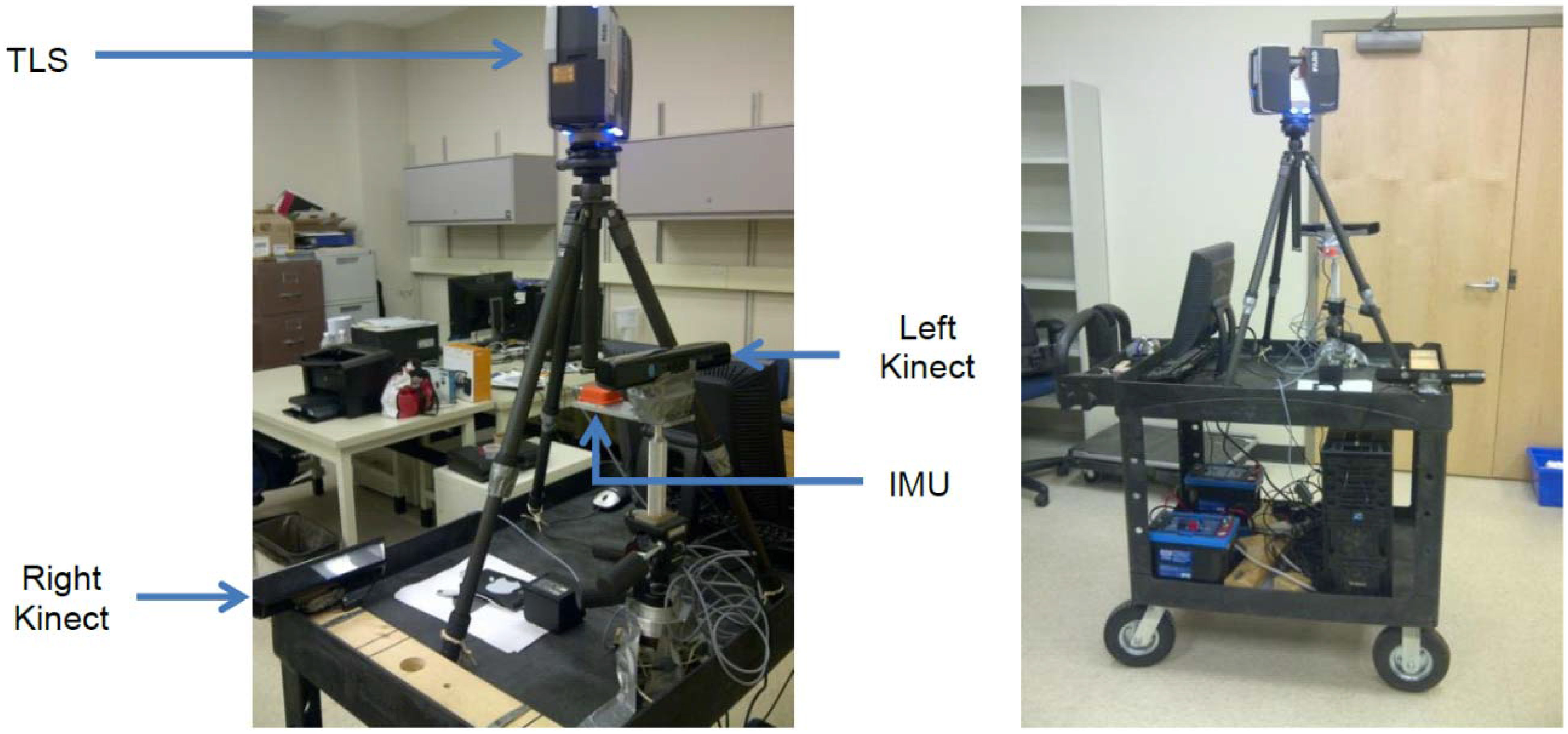
  • A novel design for a “continuous stop-and-go” indoor mapping system by fusing a low-cost 3D terrestrial laser scanner with two Microsoft Kinect sensors and a micro-electro-mechanical systems (MEMS) inertial measurement unit (IMU);
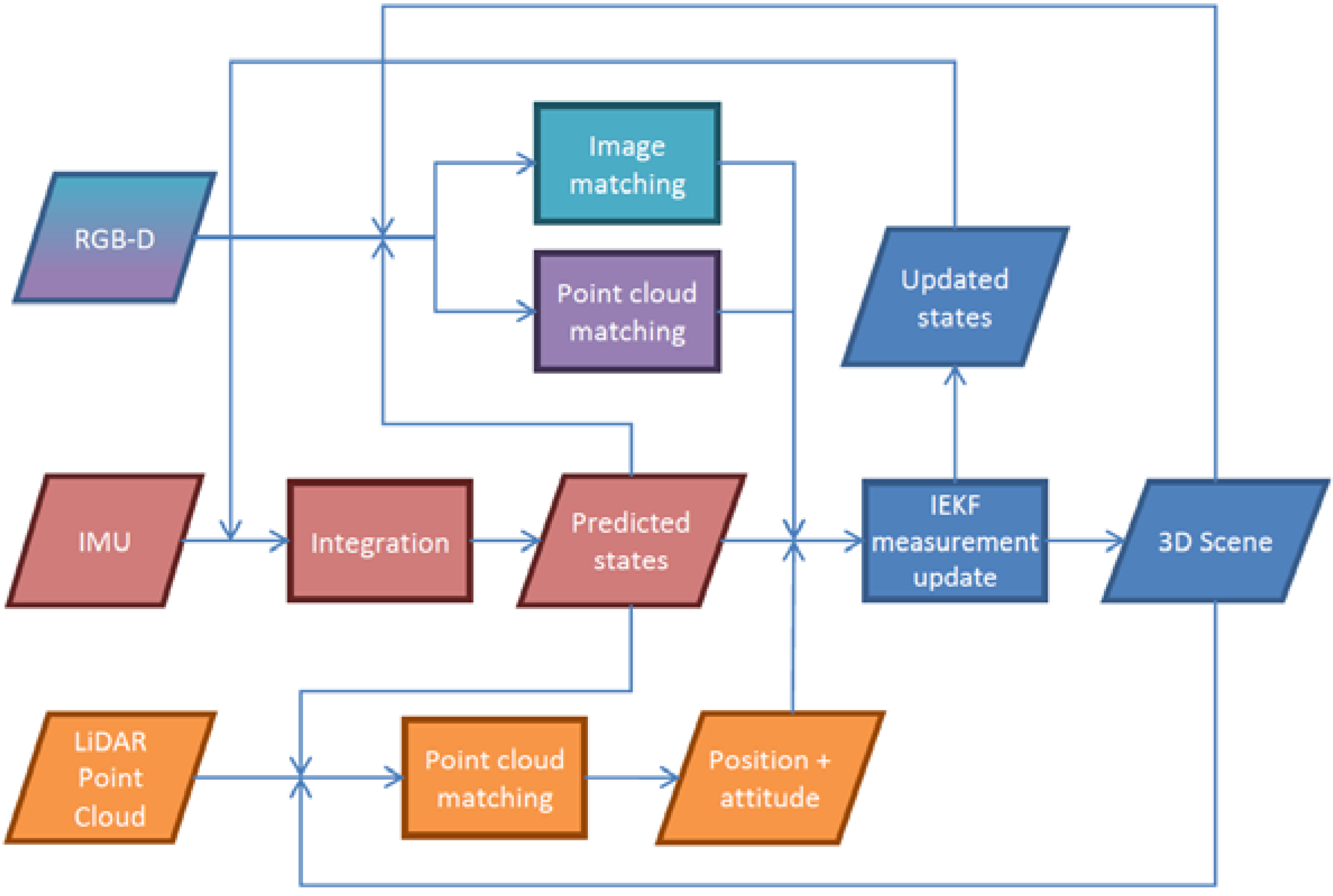
  • A solution to the 5-point monocular visual odometry (VO) problem using a tightly-coupled implicit iterative extended Kalman filter (IEKF) without introducing additional states; and
  • A new point-to-plane iterative closest point (ICP) algorithm suitable for triangulation-based 3D cameras solved in a tightly coupled implicit IEKF framework.
Before describing the proposed system, recent scientific advancements in the three key topics are first highlighted. The advantages of the proposed indoor mapping system in the same three aspects relative to existing systems are then presented. The proposed mathematical model for separately updating the IEKF-SLAM using the RGB and depth information is explained. This is followed by results from real data captured with the Scannect.

1.1. System Design

For a lot of mobile robotic operations, efficient perception and pose estimation are critical. This motivated the design for most systems to function in full-kinematic mode, where the mapping operation is performed while the robot is moving [9]. More often than not, the robot’s along-track movement extends the imaging sensor’s coverage beyond its field of view [10]. However, because of imperfections in synchronization, pose estimation, control, and other sources, the resulting map accuracy and resolution can be rather poor. To quantify the mapping errors, a reference map is often captured in stop-and-go mode where the imaging sensor is only activated when the platform has halted its movements [11]. It is agreed for terrestrial applications that perception data captured while the platform is stationary can yield higher quality data because motion blur and any other robot motion induced errors are avoided [12]. Based on a recent survey done by [12] existing mobile mapping systems either solely operates in stop-and-go or in full-kinematic mode. The former approach is hindered by the slow data acquisition and the latter may lack accuracy. This survey further indicated a system that can operate in both modes has not yet been developed; specifically one that can capture higher density, stability and accuracy data when it is parked and lower quality but continuous data while it is moving.

1.2. Choice of Sensors

Indoor SLAM can be performed using many different sensors, for example it can be applied to Wi-Fi positioning [13]. However, due to the effectiveness and wide success of optical systems for mapping, vision-based SLAM is by far the most common scheme [14]. Popular sensors used for visual SLAM include monocular/stereo cameras [15,16], 2D/3D Light Detection and Ranging (LiDAR) systems [11,17], and 3D cameras [18], all of which have their own advantages and disadvantages.
Monocular cameras are passive sensors that can capture a 2D array of light intensity information instantaneously. Although they are sensitive to the ambient illumination and the information they encapsulate for SLAM is dependent on the scene’s texture, being a bearing-only sensor [19] it is largely independent of the object’s reflectance properties and can observe details as far as their pixel resolution allows. Stereo cameras can further perceive depth from a single exposure station based on triangulation, a process similar to how human vision operates [20]. LiDAR systems on the other hand are active sensors that acquire 2D scan lines by measuring distance (based on the time-of-flight principle) and bearing information point-by-point at high speed. The third dimension is obtained either by the platform’s trajectory (for 2D scanners) or by a rotating head/mirror (for 3D scanners). They can observe dense geometric information over homogeneous surfaces under any illumination conditions. However, their observable range is hindered by the amount of energy they can emit and receive after the laser signal has been reflected and absorbed along its path. In addition, since 2D scan lines are acquired sequentially, the time it takes to sweep the laser over the object of interest is typically long, making them slower than cameras [10].
These complementary characteristics of LiDAR and imagery have been detailed and harvested for airborne and terrestrial mapping by many [21,22]. In recent years, 3D cameras have emerged integrating the benefits of time-of-flight (ToF) measurements with the fast acquisition and gridded structure of digital images at the hardware level. Despite the fact that many commercial 3D cameras are based upon the ToF principle, currently the most widely used 3D camera on the market is the structured-light RGB-D camera known as the Microsoft Kinect. The per pixel metric depth data enhances the information content of the RGB image significantly and can make tasks like obstacle avoidance, object tracking and recognition more robust and accurate [23]. While it appears that RGB-D cameras may have eliminated the need for LiDAR in robotic applications, LiDAR has retained its place in the robotics community [24], and among others, due to the limited range, resolution, accuracy, and field of view of modern RGB-D cameras. Instead, RGB-D cameras might be more suitable for filling in gaps in the LiDAR point cloud at close-range as it can be more efficient for covering occluded areas [25]. In addition, even though the cost of a Kinect is lower than most 3D ToF cameras, [26,27,28] have shown that the Kinect can produce more accurate results and are suitable for mapping; at close-range (less than 3.5 m) its accuracy can be similar to LiDAR and medium-resolution stereo cameras [26,27].
Existing indoor mapping systems based on the Kinect have so far been limited to a single system. In addition, they are often treated as substitutes for more expensive scanners, rather than being used as an aiding sensor to laser scanners. Furthermore, the integration of geometrically accurate LiDAR, semantic RGB, and efficient depth map for more informed mapping and pose estimation has not been thoroughly investigated, despite their known complementary characteristics.

1.3. Methods for Localization and Mapping

Indoor localization-only solutions exist, for example pedestrian navigation devices [29]. Often IMUs are used in conjunction with a spatial resection based on bearings, distances, or a combination of both from primitives [30]. The primitives can be points, higher-dimensional 2D/3D geometric features (e.g., lines, planes, cylinders, and spheres), or more complex surfaces (e.g., a sofa and statue of a lion). The main assumption is that the positions of the primitives are known, either from a computer-aided design (CAD) model, surveying, or other means.
On the contrary, mapping-only solutions are also common, and are typically based on bearings, distances, or both measurements from one or more locations. In this scenario, the location of the sensor needs to be known, and often in combination with orientation information [10].
Localization and mapping are highly correlated and are often described as the “chicken and egg” problem [31]. Naively performing mapping operations after localization without any accounts for their correlation can lead to poorer accuracy, or even divergence in the solution [3]. Therefore, state-of-the-art methods usually solve the two problems simultaneously using optimizers such as least-squares, Kalman filters (KF), information filters, and particle filters [32]. The measurement models used by these optimizers depend on the data source and the features being matched.
For 2D camera images, popular matching methods include area-based matching (e.g., normalized cross-correlation), point-based matching (e.g., blob detectors like scale-invariant feature transform (SIFT) or corner detectors like Harris), and line-based matching. Keypoint matching is usually more accurate than area-based methods [33], and these points can be tracked over consecutive frames (e.g., by the Kanade–Lucas–Tomasi (KLT) feature tracker) for efficiency and reliability at the risk of experiencing tracking drift. Usually a pin-hole camera model is used to relate pixel observations to their homologous point in the world coordinate system using the collinearity condition [20]. For cameras the matching in general can be formulated as 3D-to-3D, 3D-to-2D, or 2D-to-2D matching, with the accuracy and complexity generally increasing in the order presented [33].
To match point clouds from 3D cameras or laser scanners, point-based, feature-based (e.g., lines, planes, and tori), and freeform matching (e.g., ICP) are possible. Since dense point clouds are usually available and the nature of objects/shapes in the scene can be unpredictable, freeform matching is one of the most popular choices in robotics. It is very flexible but is less robust than matching signalized markers, and can be computationally intensive. The two original ICP implementations that are still widely used today are the point-to-point ICP by Besl and McKay [34] (conventionally solved using Horn’s method [35]) and the point-to-plane ICP by Chen and Medioni [36] (formulated as a least-squares minimization problem). To improve the algorithm, over the years many variations of ICP have been proposed and tested. For more details, the reader can refer to taxonomy of ICP in [37]. As no ICP algorithm is superior in all situations, the designer is responsible for selecting and/or modifying the ICP algorithm to fit their needs.
Many different VO/SLAM algorithms based on the above concepts exist and a review of all of them is beyond the scope of this paper. Instead, a few popular state-of-the-art methods relevant to this project are explained with their pros and cons highlighted.
Typical VO operates like Parallel Tracking and Mapping (PTAM) [38]. A pair of 2D images is used to intersect points in the scene with the scale being arbitrary or introduced based on a priori information. Then consecutive images that are captured use these intersected 3D points to perform a resection to solve for their egomotion. Once this transformation is known, they are once again used in the intersection process to create more points in the scene. The end result is usually a sparse map of the environment that carries little value for most mapping operations compared to dense point clouds from LiDAR or 3D cameras. Furthermore, three drawbacks arise with PTAM: (1) the “catch 22 problem” where more reconstructed 3D points give a better camera tracking solution, but cause the state vector to grow rapidly; (2) the same 3D point needs to be observable in at least three images before it can be used for tracking the camera’s motion; (3) an initial metric scale is difficult to obtain. The last two statements are less of a problem because through fusion with an IMU the scale can be estimated as quickly as 15 s [39]. Or if depth data are available it can be solved instantaneously from a single exposure and camera tracking can begin immediately following the first camera exposure [40].
Henry et al. [41] had a single PrimeSense RGB-D camera carried by a human in a forward-facing configuration for indoor mapping. They explained that the depth data ignores valuable cues in the RGB images and RGB images alone do not perform well in dark and sparsely textured areas. Therefore they presented 1-step and 2-step matching methods that exploit both pieces of information. In the 1-step case, a joint optimization was performed that minimized the point-to-point distances for the detected 3D keypoints and point-to-plane distances for the depth maps using ICP. To improve the speed of the algorithm, they suggested splitting this into two steps: running the keypoint matching first and only performing ICP after if the match was poor (e.g., insufficient keypoints were matched). This resulted in only minor compromise in terms of accuracy. In both cases, they performed RANSAC on the 3D keypoints for the initial alignment step. Compared to their previous work [42], they have replaced SIFT with the Features from Accelerated Segment Test (FAST) detector, minimized the reprojection errors of the matched 3D keypoints instead of Euclidean distances, and did a global optimization using sparse bundle adjustment (SBA) instead of the Tree-based netwORk Optimizer (TORO) [31]. In their indoor mapping experiment, they travelled over 71 m in an office space and their ICP-only solution showed 15 cm error, while their proposed RGB-D ICP method showed 10–11 cm error (i.e., 0.15% error over the travelled distance). Their proposed RGB-D ICP scheme eliminated the need to weight the color space relative to the Euclidean space [43], but created the new problem of having to weight 3D keypoints against the point-to-plane ICP. In this paper they give the two different point matches the same weight in their joint-optimization. Moreover, they only mention the possibility of weighting the points in ICP based on distances, normal angle, etc. to improve the matching but the same weight was assigned to all points. The authors acknowledge and stress the importance of minimizing reprojection errors, but their point-to-plane ICP did not adopt this scheme, only the 3D keypoints used this cost function. They also mention that because they tightly-coupled depth and color information, whenever the depth sensor is out of range they do not have 3D keypoints for RANSAC matching even though they were detectable in 2D. This can be rather common with their single forward facing sensor configuration. For example, when looking down a hallway, the majority of the center pixels will likely be out of range.
The Kinect is capable of delivering 9.2 million points per second, a rate that far exceeds any terrestrial laser scanners. A popular method for handling this vast amount of data in real-time is the KinectFusion solution [44]. They parallelized the point-to-plane ICP algorithm to be executed on the graphics processing unit (GPU) for speed and fused the dense point clouds using the Truncated Signed Distance Function (TSDF) [45]. This novel implementation was considered for this project but at the time its measurement volume was restricted by the memory of the GPU. Even with a lower resolution for the TSDF, mapping over hundreds of meters in distances was not possible. This method can map in the dark because only the depth images were considered and all the semantic RGB data were ignored. Although it was designed for handheld sequences, slow and steady egomotion was assumed, as sudden jerks and insufficient overlap can cause the ICP to fail. In addition, a lack of geometry in the scene (a well-known problem with ICP) makes it difficult for the KinectFusion method to converge to the global minimum.
More recently [46] has lifted this limitation of measurement volume by downloading the old data onto the central processing unit (CPU) and using a moving TSDF to only map the most recent and immediate point clouds. In their later paper they even took advantage of the RGB information [47], and added loop-closure [48]. Keller et al. [49] improved upon KinectFusion by replacing the volumetric representation by a point-based representation of the scene. This eliminated many computational overheads and conversions between different scene representations, making it more scalable and faster. Each point in the depth map is projectively associated with the scene and reliable points are merged using a weighted average. Besides being able to map larger areas, the biggest improvement is the ability to handle a certain degree of dynamics in the scene. Even with these significant improvements, being a single Kinect system, its field of view (FOV) is limited to less than 60° and their ICP algorithms will fail when the scene lacks features (e.g., only a single homogenous wall is in view). Also, the timing error between the color and depth information was usually neglected [50].
Leutenegger et al. [51] tightly-coupled a stereo-camera with an IMU using keyframe-based nonlinear optimization instead of filtering techniques. Keypoints were identified using the Harris detector and descriptions were computed using BRISK. Unlike the Kinect, only a sparse 3D map was obtained and landmarks were removed in the marginalization step to reduce the computation load.
Unlike the above papers, another stream of research used Kalman filtering to solve the SLAM problem. Li et al. [52] demonstrated that the performance and convergence of SLAM is affected by landmark initialization uncertainty and linearization error. The former can be addressed by using the depth information provided by the Kinect to better initialize the 3D landmarks. The latter can be improved by replacing the extended Kalman filter (EKF) with the IEKF, which re-linearizes the measurement model by iterating an approximate maximum a posteriori estimate around the updated states rather than relying on the dynamics model. They showed using real data from their keypoint based SLAM that in some situations where EKF will fail, the IEKF would not. They also proposed a way to add and remove landmarks from the state vector to avoid memory overload. The IEKF can help reduce the effect of non-linearities in the measurement model; however just like the EKF they are still based on a measurement model where a single observation is expressed as a function of the unknown states.
Aghili et al. [53] realized the importance of initial alignment for the ICP and attempts to keep track of the pose when good measurement updates were unavailable. They solved this by fusing the ICP pose in a KF under a closed-loop configuration. In this case, the measurements were loosely-coupled and the EKF only provided an initial guess for the ICP method. With a similar motivation, Hervier et al. [54] fused the Kinect with a three axes gyroscope for improved mapping and localization accuracy. They used the ICP algorithm in the Visualization Toolkit (VTK) to first solve for the pose, and then fuse it in the KF in a loosely-coupled manner. In their current system, they mentioned it is difficult to evaluate movements parallel to a flat wall.
In the navigation domain, vision-assisted IMU is popular for localization in GNSS-denied environments, but the reconstructed scene is often viewed as a nuisance parameter. Kottas and Roumeliotis [55] presented results from monocular camera and IMU fusion that used both point and line features. Their proposed Observability-Constraint Multi-State Constraint Kalman Filter improved the consistency of the EKF results by ensuring rotational information about line, which is unobservable by vision, does not enter the filter. Using this method for a handheld sequence, they estimated sparse feature parameters and reported a localization error of 0.31 m over a 144 m trajectory (i.e., 0.22% error of the distance travelled). Li et al. [56] fused the IMU and rolling-shutter camera onboard the Samsung Galaxy S2 for pose estimation. Using their modified Multi-State-Constraint Kalman Filter a sliding window of camera states was processed and an approximate positioning error of 0.8% over the travelled distance was reported.
All these SLAM solutions will fail in cases when a single homogenous plane is imaged. Often when the ICP method is used with a KF, they are loosely-coupled rather than tightly-coupled. Most of the work either ignores the RGB information or if included they require the depth and RGB information to be available simultaneously and assumed no synchronization errors.
In Grisetti et al. [31] they distinguished SLAM into the filtering approach and smoothing approach. Filtering approaches are incremental by nature and often use KF (also referred to as online SLAM), whereas smoothing approaches estimate the complete trajectory from all the measurements (a.k.a the full SLAM problem). This paper focuses on the forward filtering part of SLAM and proposes new ways to solve monocular VO and ICP in a tightly-coupled KF.

2. The Scannect Mobile Mapping System

The Scannect is an indoor mapping system that is unique in its System Design, Choice of Sensors, and Methods for Localization and Mapping. Each of these aspects of the Scannect is explained in the following sections.

2.1. Proposed System Design

The proposed system attempts to harvest the accuracy and stability of stop-and-go systems while maintaining a degree of speed from full-kinematic systems. High quality 3D scans are captured when the robot has “stopped”, and lower quality data is captured while it is “going” for mapping and keeping track of the relative change in pose. For this reason, the system design can be seen as a hybrid between static and kinematic mapping, termed continuous stop-and-go mode in this paper. According to a recent review by [12], systems operating in continuous stop-and-go mode have not yet been released. If higher quality data are desired the robot can make more frequent stops, hence approaching the stop-and-go solution’s quality or if speed and time is of the essence, it can make zero stops (approaching the full-kinematic solution). This trade-off between speed and accuracy does not affect other components of the Scannect, and can therefore be easily adapted to the project at hand.

Designed Robot Behavior

The robot’s behavior during the mission is described in the following stages with the desirable trait of the system highlighted:
  • Stage 1: The robot enters an unfamiliar environment without prior knowledge about the map or its current position.
    The absolute position may never be known, but an absolute orientation based on the Earth’s gravity and magnetic fields is determinable.
    The system should “look” in every direction to its maximum range possible before moving around to establish a map at this arbitrary origin.
  • Stage 2: Due to occlusions and limited perceptible range, the robot needs to move and explore the area concurrently.
    When exploring new areas the map should be expanded while maintaining the localization solution based on the initial map.
  • Stage 3: Occasionally when more detail is desired or the pose estimation is uncertain, the system can stop and look around again.
    As the system is for autonomous robots with no assumptions about existing localization infrastructure (e.g., LED position systems), every movement based on the dead-reckoning principle will increase the position uncertainty. Typically it is more accurate to create a map using long-range static remote sensing techniques because they are typically less than the dead-reckoning errors.
    Looking forward and backward over long ranges from the same position can possibly introduce loop-closure.
    One of the Kinects and the IMU are rigidly mounted together and force centered on the mobile platform. Through a robotic arm, quadcopter or by other means the Kinect and IMU can be dismounted from the platform during “stop” mode for mapping, making it more flexible/portable for occlusion filling. Afterwards it can return and dock at the same position and orientation and normal operations is resumed.

2.2. Proposed Choice of Sensors

The starting point of the Scannect is the FARO Focus3D S terrestrial laser scanning (TLS) instrument. This is motivated by the accuracy, stability, speed, range, and field of view of this modern static 3D TLS instrument, (e.g., millimeter-level range accuracy and 360°/310° horizontal/vertical FOV, respectively). This sensor is very suitable for indoor mapping applications, especially with the recent upgrades (i.e., digital compass and tilt sensors), and reductions in cost, size, and weight. Its success for indoor mapping can be seen in the papers published using this system for as-built surveys and cultural heritage documentation [57,58].
The Microsoft Kinect is a trinocular vision system capable of capturing dense RGB-D information at up to 30 Hz. The RGB information comes from an onboard VGA resolution camera while the depth information is determined using the coded-light principle: a pattern is emitted by the projector and simultaneously imaged by the infrared (IR) camera to perform photogrammetric intersection. More details about the Kinect can be found in many articles, e.g., [59,60].
In large open spaces (e.g., a gymnasium, shopping malls, and airports) TLS can be more efficient and effective at mapping than 3D cameras like the Kinect. However, TLS falls short when many occlusions exist in the scene because so many static scans are needed for complete coverage, which is very time-consuming. When setup on a mobile platform (e.g., trolley) the setup-move-setup time is reduced [12]. A selective FOV in theory can shorten the scan time when compared to a full 360° scan, however because of the rapid scan speed of modern scanners, the process of capturing a preview scan followed by the manual FOV selection and doing a dense scan can actually result in longer overall acquisition time. In cases where small occlusions needed to be filled, the Kinect is perhaps more efficient. Unlike 2D profile scanners which essentially have no overlap in kinematic mode, the Kinect provides a 3D point cloud within its FOV instantaneously at 30 Hz. Consequently, a high-degree of overlap exists between consecutive frames, which facilitate continuous point cloud stitching for higher quality mapping while maintaining the robot’s pose. Because the Kinect, as well as other 3D cameras currently on the market, all have a relatively small FOV (the largest being 90°), a simple and cost-effective solution is to add extra Kinects [61].
The Scannect was equipped with two sideward facing Kinects (Figure 1); this architecture was chosen to maximize the overall FOV for indoor SLAM and to prevent possible interference between the two Kinects. If desired, additional Kinects are possible and the interference issue can be mitigated by introducing small vibrations to each Kinect [62]. Although a forward facing and skyward facing Kinect design has also been considered, it was not implemented because (1) a forward facing Kinect usually does not have sufficient range to reach the end of a long corridor to provide any useful information; (2) the considered situations in this paper assume a flat horizontal floor for the building, which is often the case, so a non-holonomic constraint was used for constraining the height of the robot instead since a sideward facing Kinect is more valuable for mapping.
Nonetheless, all the sensors discussed thus far require a direct line-of-sight to conjugate features in the overlapping regions. If the overlap between two visual datasets is small or lacking in features/texture, optical-based matching techniques may be inaccurate or even fail in some cases. A suitable aiding device is an inertial measurement unit, which operates well regardless of its environment. A MEMS-based IMU from Xsens, the MTi, was adopted for the task at hand. When the robot enters a dark corridor with walls too far for the Kinect, the integrated rotation rate will keep track of the orientation, and the rotated acceleration after double integration will keep track of the position of the platform.
Figure 1. Sensor configuration of the Scannect.
Robotics 03 00247 g001
All data were logged and processed on a Windows 7 desktop computer equipped with an Intel® Core™ i7 processor (up to 3.07 GHz) and 12.0 GB of RAM. In this prototype, the processing was performed offline, which is not unreasonable as most stop-and-go mobile scanning systems process their data post-mission.
Overall, the Focus3D S is envisioned for mapping large open areas in static mode. When the robot is moving the Kinects are used for localization and filling in the shadowed areas until the system stops to perform Zero velocity UPdaTes (ZUPT) and capture another laser scan. The IMU continuously assists the Kinect matching and bridges the gaps when vision-based localization fails due to lack of details in the scene. To the authors’ best knowledge this is the first paper using more than one Kinect for an inside-out type system. Popular multi-Kinect systems are designed for body scanning or motion capture with an outside-in design [61]. Furthermore, the Kinect is usually used as the sole mapping sensor, instead of playing a more assistive role to a more accurate laser scanner, as in this paper.

System Calibration

Systematic errors are prevalent in all man-made instruments, for instance due to manufacturing flaws. Before integrating the four proposed sensors for SLAM, they were first individually calibrated for their intrinsic parameters. Afterwards, the relative rotation (boresight) and relative translation (leverarm) between all the sensors were determined through an extrinsic calibration process. Only the intrinsic calibrations of the optical sensors are considered in this paper. The calibration procedure for MEMS-based IMUs has reached a level of maturity that is widely accepted [63]. The commonly adopted methods solve for biases, scale factor errors, and axes non-othogonalities for the triad of accelerometers and gyroscopes, and misalignments between them. For the accelerometer calibration, the sensor can be placed in various orientations and capturing a sequence of static data. These measurements are related to the local gravity vector, which is used as the reference signal. For the gyroscopes, a rotation rate table can be used to establish the reference signal. Since such a calibration requires specialized equipment that is not easily accessible, the manufacturer’s calibration was relied upon. Furthermore, MEMS IMUs are known to have a poor bias stability, so the residual systematic errors need to be modeled stochastically in every operation.

Microsoft Kinect RGB-D Camera Calibration

The Kinect is originally intended for gaming applications, where metric measurements are not critical. In order to integrate the Kinect with a laser scanner for mapping, the sensor needs to be individually calibrated to ensure the residual systematic errors from the manufacturer’s calibration are minimized. Distortions in the Kinect’s depth map have previously been reported and various calibration approaches have been proposed [59,64]. As the Kinect is a relatively new sensor, a commonly accepted calibration procedure has not yet been established, which is in contrast to MEMS IMU calibration. For convenience, a user-self calibration approach that requires only a planar checkerboard pattern for performing a total system calibration was selected.
The Kinect consists of three optical sensors, all of which can be modeled using the pin-hole camera model. The well-established bundle adjustment with self-calibration method was modified in [65] to solve for all the intrinsic and extrinsic parameters of all the optical sensors in the Kinect simultaneously. This method was adopted in this paper and was responsible for independently calibrating the two Kinects installed onboard the Scannect. The results from the calibration are published in [65].

FARO Focus3D S 120 3D Terrestrial Laser Scanner Calibration

The Focus3D S is the lowest-cost sensor in its category of laser scanners. Compared to more expensive scanners within the same class, it has been found to exhibit more significant systematic distortions, in particular angular errors. The multi-station self-calibration approach is a popular and effective means for reducing the systematic errors internal to TLS instruments without the need of specialized tools [66,67]. Analogous to camera calibration, by observing the same targets from different stations a least-squares adjustment can be performed for solving the biases in its distance and bearing measurements and various axes misalignments, eccentricities, and wobbling. Recently, [68] showed that signalized targets can be replaced by planar features to achieve similar calibration results with reduced manual labor. The Focus3D S on the Scannect was calibrated using this plane-based self-calibration method, and the calibration results can be found in [69].

Boresight and Leverarm Calibration between the Kinect and Laser Scanner

Both the Kinect and laser scanner are visual sensors, therefore target fields such as a planar checkerboard pattern is visible to both. These common targets can be independently extracted in their corresponding point clouds and then related through a 3D rigid-body transformation [70]. This approached was adopted to simultaneously solve for their boresight and leverarm parameters. Since the Kinects point away from each other, they were related through the intermediate laser scanner.

Boresight and Leverarm Calibration between the Kinect and IMU

The problem of solving for the 3D rigid body transformation parameters between an IMU and camera is often encountered in multi-sensor mapping systems [10]. Some common methods include simple surveying techniques via a total station, solving it as a state estimation problem in an EKF, or formulating it as an offline global optimization problem. The first method is most suitable for higher-end IMUs and metric cameras with clear markers on the exterior casing, for instance in airborne mapping systems. The locations of the Kinect’s perspective centres are unknown and CAD models are not published by Microsoft. Therefore, the other two algebraic calibration methods are perhaps more suitable.
Lobo and Dias [71] proposed a popular two-step calibration procedure that first estimates the boresight parameters and then uses a turntable that spins about the IMU’s origin to solve for the leverarm parameters. Not only does this require specialized tools and careful placement of the system on the turntable, correlations between the rotational and translational parameters are ignored in this method. Hol et al. [72] formulated the calibration as a gray-box model where the navigation states were solved in the EKF using their current best estimate of the unknown parameters (boresight, leverarm, gyro bias, accelerometer bias, and gravity vector). A post-filtering adjustment was then used to improve their estimate of the unknown parameters simultaneously by minimizing the differences between the predicted and measured target positions in image space. This online filtering and offline adjustment is then repeated until convergence. This type of calibration is preferred in this project because it is more user-friendly and can account for the correlations between the boresight and leverarm parameters. Based on the approach in [72], the measurement model shown in Equation (1) was used for calibration in this project. Two subtle differences exist in the implementation presented herein: first, the slowly time-varying biases are solved in the IEKF like [73]; second, the gravity vector in the navigation frame has been replaced by the rotation angles between the navigation frame and world frame of the checkerboard. The rotation matrix notation was used here and in other equations for convenience in representation; in the actual adjustment, quaternions were used to give the system full rotational freedom without encountering gimbal lock.
Robotics 03 00247 i001
where Robotics 03 00247 i002 is the observation vector for point i expressed in the RGB image space at time t; Robotics 03 00247 i003 is the scale factor for point i at time t (which can be eliminated by dividing the image measurements model by the principal distance model [20]); Robotics 03 00247 i004 is the relative rotation between the IR and RGB cameras; Robotics 03 00247 i005 is the relative rotation between the IMU sensor and IR camera; Robotics 03 00247 i006 is the orientation of the IMU sensor relative to the navigation frame at time t; Robotics 03 00247 i007 is the relative rotation between the world frame defined by the checkerboard and the navigation frame; Robotics 03 00247 i008 is the 3D coordinates of point i in the world frame; Tn (t) is the position of the IR camera in the navigation frame at time t; Δbs is the leverarm between the IMU sensor and IR camera; ΔbIR is the relative translation between the IR and RGB cameras.

2.3. Proposed Methods for Localization and Mapping

Figure 2 shows the interaction between the sensors onboard the Scannect. The different colors separate the various components of the Scannect (e.g., cyan highlights the egomotion estimation using RGB images and purple highlights the 3D image processing). The IMU observations after correction (Equation (2)) were integrated to provide changes in orientation and position (Equation (3)), which were useful for initializing the 2D/3D matching and keep track of the states between measurement updates. The accelerometer and gyroscope biases were solved in the KF as a first order Gauss-Markov process (Equation (4)). The Gauss-Markov parameters were determined from autocorrelation analysis [74]. The TLS point clouds were matched using the conventional point-to-plane ICP [36] with the first point cloud oriented relative to magnetic north in the local level frame. The proposed RGB-D localization and mapping method is based on a novel ICP implementation suitable for triangulation-based 3D cameras such as the Kinect. The new cloud was always registered with the global scene to partially address the loop-closure problem. The localization was separated into depth-only and RGB-only for two reasons: (1) the depth and RGB streams are not perfectly synchronized; and (2) the depth measurements have a limited range—by processing the RGB data separately, localization of the robot is still possible when depth data are unavailable. Both depth-only and RGB-only processing used a tightly-coupled implicit iterative extended Kalman filter to estimate the states.
Figure 2. The overall workflow of performing Simultaneous Localization and Mapping (SLAM) using the Scannect.
Robotics 03 00247 g002
Robotics 03 00247 i009
Robotics 03 00247 i010
Robotics 03 00247 i011
where xn, n, and ẍn are the position, velocity, and acceleration of the IMU sensor in navigation frame, respectively; fs (t) and Robotics 03 00247 i012 are the accelerometer and gyroscope measurements at time t, respectively; εa (t) and εω (t) are their corresponding measurement noises; Robotics 03 00247 i013 is the rotation rate of the earth as seen in the navigation frame; gn is the local gravity in the navigation frame; qs→n the rotation from IMU sensor frame to navigation frame expressed using quaternions; δa (t) and δω (t) are the slowly time-varying accelerometer and gyroscope biases, respectively, which are modelled as a first order Gauss-Markov process; ηa (t) and ηω (t) are the corresponding Gauss-Markov process driving noises; and Δt is the time interval between the current and previous measurement.

2.3.1. Tightly-Coupled Implicit Iterative Extended Kalman Filter

The Kalman filter has been a popular choice for sensor fusion and navigation for decades. The Kalman filter assumes a linear relationship between the measurements and the states. Non-linearities can be approximated by using a first order Taylor series expansion. If the non-linearities are severe, higher order terms of the Taylor series can be included, and/or an iterative approach can be taken. All the filtering in this paper was done following the latter approach where an IEKF is used for updating the states [75]. A total of 16 states were used by the system (namely 3 for position, 3 for velocity, 4 for attitude in the quaternion, 3 for gyro bias, and 3 for accelerometer bias) and the size of this vector remains constant throughout the entire large-scale mapping project. This is desired and done to reduce the likelihood of divergence with a large state vector, and the reduction of system performance over time as more states are added [75]. In addition, many geometrical formulas used in vision actually violate the parametric model assumed by the KF (i.e., a single observation is a function of the unknown states, as shown in Equation (5)); instead they are implicitly defined (i.e., the observations and unknown states are inseparable in the measurement update model, as shown in Equation (6)). The extension of the conventional IEKF for implicit math models are given in [76], and was used in all the matching processes described in this paper.
y = h(X)
h(X,Y) = 0
where y represents a single observation; Y represents multiple observations; X represents the unknown states; and h denotes a functional model relating the observation(s) and unknowns.
For outlier removal, the normalized residuals were used instead of testing the innovations [77]. This implicit IEKF formulation permits the Kinect measurements to update the state vector in a tightly-coupled manner, which allows for the system to be updated even if the matching is underdetermined (e.g., less than the minimum number of matches is found, or their distribution is collinear).

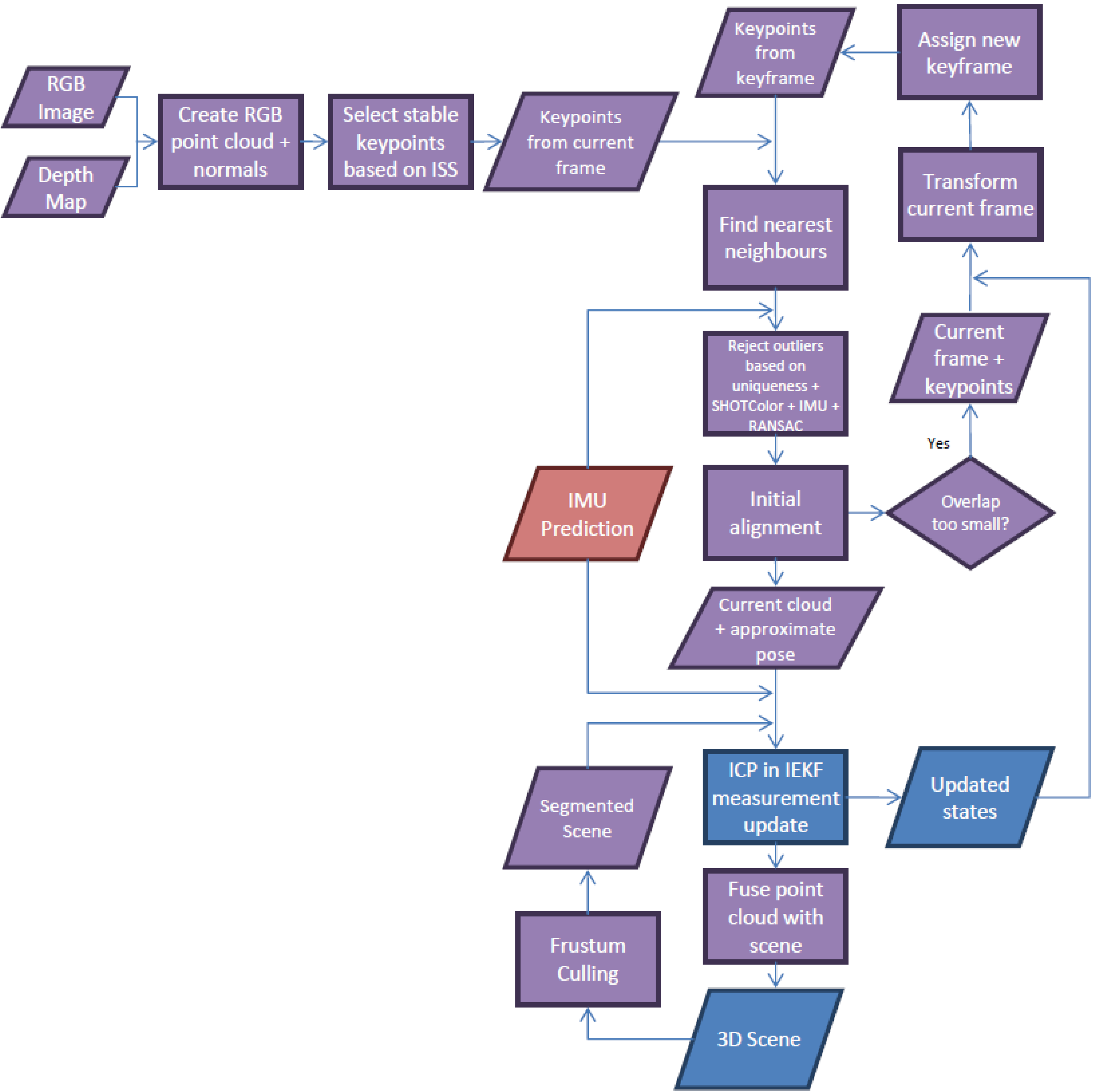
2.3.2. Dense 3D Point Cloud Matching for the Kinect

Computer vision techniques for egomotion estimation and 3D reconstruction are very suitable for robotics SLAM applications because of their balance between speed, accuracy, and reliability. Often in freeform scan-matching, the ICP method is used. The ICP matching is usually first solved independently to reconstruct the scene, and then the relative translation and rotation between the point clouds are fused using a Kalman filter to update the pose. When the point clouds being matched are rich in geometric features, this method can provide high quality pose estimates. Typical indoor urban environments present additional challenges such as a single flat wall and sparse/poorly-distributed point clouds due to sensor saturation (the Kinect has difficulties producing a point cloud under direct sunlight, even through windows) and scene’s reflectivity (e.g., mirrors and glass). For the former case, point-to-point ICP can converge to an infinite number of solutions based on the initial alignment, and the point-to-plane ICP will have a singular matrix that would not invert due to lack of geometric constraints. If the wall exhibits a lot of texture, RGB information can be combined with the standard geometry-only ICP in a joint optimization to obtain a solution [43], however if the wall is homogenous (e.g., white walls without textures are common) this approach is not applicable. Furthermore, based on the OpenNI programmer’s guide [78] the depth and color streams of the Kinect are not perfectly synchronized. In some extreme cases, data captured using Kinect Studio from the Microsoft Kinect SDK even revealed significant lag between the two streams. Figure 3 shows the temporal availability of color and depth information while a Kinect was logging both simultaneously. The red and blue lines indicate when a RGB image and depth map was captured, respectively; lag up to 0.26 s can be observed.
Figure 3. Recorded color and depth data using Kinect Studio with the red and blue lines showing the time when an image is acquired.
Robotics 03 00247 g003
A general overview of the depth matching methodology is summarized graphically in Figure 4. A calibrated point cloud augmented with RGB and normals was generated in near real-time using OpenMP, Point Cloud Library (PCL), and [65]. Despite the synchronization errors, the out-of-sync color information was included in the initial alignment step to improve the distinctiveness of the selected keypoints. The stable keypoints were then extracted from this new point cloud and matched to a previous keyframe. The estimated pose after outlier removal (using the uniqueness constraint, Signature of Histograms of OrienTations COLOR (SHOTColor) descriptor, IMU predicted image point locations, and RANSAC) was used as the initial alignment for the tightly-coupled ICP. During scan-matching, the input point cloud (without considering the RGB information) was iteratively matched with the reconstructed scene (i.e., the map) while incorporating the a priori information from the IMU. The synchronization problem was mitigated by using the measurement model described in the section Cost Function, which updates the KF using solely the geometry information. After a laser scan, when mobile mode was resumed, this approach becomes comparable to a localization only solution in a known environment until reaching occluded areas. The output of this method includes the 16 updated states and an extended map of the environment. The state parameters were estimated in the KF, while the map was obtained from averaging new points at the current pose with the scene using a voxel grid. The adopted model-to-scene scan-matching approach estimates the map by allowing the scene to be updated through a moving average instead of augmenting the state vector with the map, which is computationally demanding for the KF since every Kinect exposure contains up to 307,200 points.
Figure 4. SLAM using the Kinect’s depth information.
Robotics 03 00247 g004
The central concept of the proposed depth processing pipeline is the ICP algorithm. Numerous variations of ICP can be found in literature, each with their own advantages and disadvantages. Rusinkiewicz and Levoy [37] summarized five key components for tuning the ICP algorithm: the sampling method, searching, cost function, outlier rejection, and weighting. Following this guideline, a new point-to-plane ICP solved in a tightly-coupled IEKF is proposed to account for the solo homogenous flat wall situation described above. Through the additional information provided by the dynamics model, not only does the initial alignment become trivial, it makes the single plane case solvable. The following sections explain the proposed ICP algorithm in relation to the five key components, initial alignment, and the loop closure problem.

Sampling

A single Kinect depth map is 640 by 480 pixels, which can result in a point cloud with a maximum size of 307,200 points. This is a lot of data, especially considering the Kinect simultaneously captures RGB images at 30 Hz. Since the corresponding points between the IR camera and projector are determined using a 9 × 9 kernel [59], depth values of adjacent pixels are highly correlated and do not carry as much information as pixels that are further away. Therefore, to reduce the computation time, the point clouds were downsampled. For this, the normal downsampling technique suggested by [37] was used, because it showed better performance than uniform and random downsampling.

Searching

The popular Fast Library for Approximate Nearest Neighbors (FLANN) [79], which is a fast KD-tree, was used for speeding up the query process, which is one of the most computationally intensive steps of the ICP algorithm. Instead of just finding a single nearest neighbor in the target cloud for every point in the source cloud, the k-nearest points in the target cloud based on the Euclidean distance to the query point were selected, and the point with the minimum orthogonal distance was chosen as the corresponding point. This was then repeated with every point in the target cloud as query points to find the correspondences. Only correspondences that pass this uniqueness constraint were considered as matches.
Instead of building a KD-tree for a growing scene and querying a large amount of points, two steps were taken to reduce the memory and the processing load. First, every new ICP-registered point cloud was fused with the scene model using a voxel grid representation, where points within the same voxel were reduced to their centroid. The second step involves a fast segmentation of the scene to extract only regions that were overlapping with the new incoming point cloud using frustum culling [80] based on the FOV of the Kinect and IMU-predicted pose. This essentially sets a threshold on the maximum number of points to be queried, thus prevented certain iterations from running significantly longer than others.

Cost Function

The point-to-plane cost function minimizes the orthogonal distances instead of the Euclidean distances as in the point-to-point ICP; this is known to perform better in terms of accuracy and convergence speed for most cases [37]. More importantly, it is preferred in this application because it would not “anchor” the along-track translation of the robot when it is travelling down a corridor. The point-to-plane ICP will only minimize the 1D orthogonal distance, therefore for a side-looking Kinect it will not prevent it from sliding along the wall as desired. When solving it in a KF framework, information from the dynamics model (i.e., IMU) can help push the solution forward in the along-track direction while the ICP corrects the across-track position and the two orientations that are not parallel to the normal of that wall. Furthermore, the proposed tightly-coupled point-to-plane ICP will not be singular even if only one plane is within view.
As for all camera-based models, minimization of the reprojection errors yields higher quality results than simply minimizing the Euclidean distances because it better describes the physical measurement principle. Following the derivations from [65], for a rigidly attached stereo camera, its measurement model can be written as Equation (7) (for the master camera) and (9) (for the slave camera), where the projector is treated as a reverse camera. The projector’s observation vector Robotics 03 00247 i014 is derived by backprojecting the 3D points into the projector’s image space using its extrinsic and intrinsic parameters [65]. The inherent scale ambiguity for both the IR camera ( Robotics 03 00247 i015) and the projector ( Robotics 03 00247 i016), which are traditionally eliminated from the model by dividing the first and second components by the third component of Equations (7) and (8) in parametric form [20], are solved through spatial intersection with the point-to-plane constraint (realized by substituting Equations (7) and (8) into Equation (9), respectively). The depth camera measurement update model implemented in the proposed KF framework is then obtained by equating Equations (7) and (8). It is worth noting that the functional relationship between the observations (i.e., image coordinate measures for the IR camera and projector) and unknown states (i.e., the pose) are implicitly defined. The math model presented here minimizes the reprojection errors of the Kinect’s IR camera and projector pair implicitly to reduce the orthogonal distance of every point in the source point cloud relative to the target point cloud.
Robotics 03 00247 i017
Robotics 03 00247 i018
Robotics 03 00247 i019
where, Robotics 03 00247 i020 is the relative rotation from the IR camera of Kinect k to the IR camera of the reference Kinect; Robotics 03 00247 i015 (t) and Robotics 03 00247 i016 (t) are the scale factors for point i observed by the IR camera and projector of Kinect k at time t, respectively; Robotics 03 00247 i021 and Robotics 03 00247 i014 are the image measurement vectors of point i observed by the IR camera and projector of Kinect k at time t, respectively; Robotics 03 00247 i022 is the relative rotation between the IR camera and projector of Kinect k; Δbk is the relative translation between the IR camera of Kinect k and the reference Kinect; Δck is the relative translation between the IR camera and projector of Kinect k; ai, bi, ci, and di are the best-fit plane parameters of point i in the navigation frame.

Outlier Rejection

The correspondence matching between two point clouds can only be seen as approximate because exact point matches cannot be assumed in dense point clouds captured by the Kinect or laser scanner. This causes the ICP algorithm to be highly sensitive to outliers in the approximated correspondences. To minimize the possibility of outliers, several precautions were taken, resulting in the following three outlier removal steps.

Rejection When Estimating Correspondences

One of the benefits of including an IMU is that it can provide good initial alignment for the ICP. Using this prediction and a fixed radius around each query point, correspondences established during the searching step above that were outside of each sphere can be removed. The remaining correspondences were further compared using their normal vector determined in their local neighborhood using orthogonal regression. Only points with differences in spatial angle less than a threshold were retained.

Rejection Using RANSAC

When more than 3 non-collinear points were matched between the source and target clouds, RANSAC based on the point-to-point ICP from Besl and Mckay [34] can be used for finding the inliers efficiently. This approach is similar to the RANSAC approach explained in [41].

Rejection in the Kalman Filtering

In case outliers still exist in the correspondences, standard outlier detection method based on the normalized residuals was adopted [77].

Weighting

Assigning weights that are inversely proportional to the depth measurements when registering point clouds coming from the Kinect has shown to have significant improvements in terms of accuracy [50]. For the Scannect this was achieved based on the pin-hole camera model and collinearity equations with assumed additive Gaussian noise for the pixel measurements, which have been shown to be capable of describing the distance measurement uncertainty of the Kinect over its full range [28]. This weighting scheme simplifies the observation variance-covariance matrix to a diagonal matrix while properly describing uncertainties in the point cloud due to the baseline-to-range ratio and parallax angle over the Kinect’s full frame. In contrast to [50], which would assign the same weight to all the points when registering coplanar points between two point clouds while the Kinect is oriented orthogonal to the wall, the adopted method will assign slightly different weights based on the variation of the parallax angles in these coplanar points. The end result is similar to the empirical weighting scheme adopted in [50], but with the underlying physical measurement principles of the Kinect expressed mathematically.

Initial Alignment

Generally, consecutive Kinect depth maps are captured merely fractions of a second after another. This plus transporting the Kinect slowly and smoothly during the SLAM process results in the initial transformation of the ICP to be highly predictable by a suitable motion model, and sometimes can even be assumed to be the same as the previous pose. Nevertheless, the IMU predictions are usually sufficient to get the ICP to converge to the correct solution because of the relatively short time update. However, because the ICP tends to converge to a local minimum as oppose to the global minimum, whenever possible the initial alignment is derived via other means to keep the ICP updates as independent from the IMU predictions as possible. This reduces the chance of a poor IMU prediction causing the ICP to converge to a local minimum and then using this distorted scene for camera localization.
This alternative method for deriving the initial alignment is based on 3D keypoint matching [41]. Similar to the conventional 2D keypoint matching technique [81], 3D keypoint matching begins with keypoint detection, every keypoint is then associated with a description, and points with the most similar description are matched. Most of the papers directly solve for the egomotion in EKF using this keypoint method, indicating its fidelity. However, in this paper they are only treated as initial approximations for ICP because a reliable implementation typically requires texture information, which as mentioned, RGB images are not triggered simultaneously as the depth images in the Kinect.
The Implicit Shape Signature (ISS) [82] was used for extracting keypoints with a unique and stable underlying surface. Many existing 3D keypoint detectors are just extensions of 2D image edge/corner detectors (e.g., Harris). While edges/corners are good for 2D images, in 3D their depth measurements are usually less reliable due to for example the mixed pixels effect. Therefore, the ISS, which was originally designed for 3D point clouds was favored. Also, it was chosen because [83] showed it has better overall performance than other 3D keypoint detectors that are publically available in PCL. To have a strong description for the detected keypoints, SHOTColor (a.k.a. Color Signature of Histograms of OrienTations (CSHOT)) in PCL was used [84]. This is one of the few descriptors that incorporates both shape and color information into their description, making its signature the most unique (i.e., highest dimension) in PCL. RANSAC was then used to select a group of inliers and estimate the initial alignment between the two clouds to be used in ICP. Since RANSAC is an expensive process, the IMU predictions were used to eliminate obvious false positives by setting a radius threshold around each keypoint.

Loop-Closure

The proposed method presented here focused only on the filtering solution, also known as the SLAM frontend. For a full SLAM solution, the global relaxation and optimization is crucial. To partially address the issue of loop closure in this paper, the ICP is carried out in a model-to-scene fashion like KinectFusion [44]. This way, every new cloud coming from the sensors was matched to the global scene. This approach can be even more effective when performing on laser scanner data because of their wide FOV and long-ranges.

2.3.3. RGB Visual Odometry

As mentioned, RGB data was processed without consideration of the depth information. This reduces errors in egomotion estimation introduced through time synchronization errors [50] and more importantly keeps track of the pose even when depth data is unavailable and/or unreliable (e.g., imaging glass) [40]. The basic assumption is that the scene is static and any changes in the appearance of the RGB image must be caused by the camera’s movement. For this task of identifying changes in consecutive images, the popular SIFT keypoints are detected along with descriptions computed by SURF using OpenCV. A blob detector is preferred over edge/corner detectors because such geometric information is already encapsulated in the depth data processing pipeline [85]. Correspondences were established by searching for points in the two images with the most similar description. These potential matches were then filtered based on uniqueness constraint, the IMU predicted keypoint positions in the new image, 5-point RANSAC in OpenCV, and later via outlier rejection at the measurement update stage. When the pixel differences between conjugate image points are smaller than a threshold ZUPT is performed, otherwise the camera measurement update is executed. The proposed VO workflow is summarized in Figure 5.
Figure 5. Visual odometry using monocular vision.
Robotics 03 00247 g005
Monocular camera trajectory estimation in general can be solved as a SLAM problem or using VO [33]. The former achieves better global consistency at the expense of higher complexity and being more computationally demanding. While the latter focuses on local consistency and has shown great success for example in the Mars Rover exploration. VO is preferred in this project because the mapping and localization are mainly achieved using ICP, while the RGB data is just an aid to improve localization when depth is not available or when traversing over highly texturized areas of the map. The proposed VO algorithm differs from PTAM in the sense that it implicitly solves for the 3D points from a pair of images. This simultaneous photogrammetric intersection and resection is mathematically realized through solving the set of linear equations in Equation (10) and obtaining an implicit functional model. This was the main motivation to choose the VO route because it is possible to formulate a 2D-to-2D matching VO so as to not increase the size of the state vector while incorporating all the camera geometry information, correlation between the pose and reconstructed points, and minimizing the reprojection errors.
Its advantages over PTAM include egomotion estimation by matching across two images instead of thrree images, no need for a recovery routine in case camera tracking fails, and it is more scalable because of the fixed state vector dimension. A noticeable disadvantage arises from the fact that reconstructed points are not memorized; in other words they are immediately forgotten in the KF and later images cannot resect from continuously improving 3D object points, but only from selected key frames.
Robotics 03 00247 i023
where Robotics 03 00247 i024 is the relative rotation between the RGB and IR camera of Kinect k; Δdk is the relative translation between the RGB and IR camera of Kinect k.

3. Results and Discussion

3.1. Boresight and Leverarm Calibration between the Kinect and Laser Scanner

Once all the optical systems were independently calibrated their measurements need to be related in 3D space before they can be tightly-coupled and fused in a KF. A standard checkerboard pattern was placed in 17 different static positions and orientations in front of one of the Kinects, where point clouds with the RGB texture overlaid were captured. At every setup, a laser scan of the checkerboard was also captured. The corners were extracted in 3D using a least-square cross-fitting [86]. The necessary boresight and leverarm parameters were then computed using the 3D rigid-body transformation equations solved in a least-squares adjustment. The same procedure was then repeated between the other Kinect and the Focus3D S. Although the two sets of boresight and leverarm parameters were defined with respect to the Focus3D S, for the convention adopted, they were redefined to use the left Kinect (mounted with the IMU) as the reference coordinate system. To assess the fit between the point clouds, 10 planes at various orientations and positions were extracted from both Kinects and compared with the Focus3D S as the reference. The RMSE computed using the orthogonal distances between the Kinect point clouds and the plane defined by the Focus3D S is 4.5 mm and 6.2 mm for the left and right Kinects, respectively. These estimates were higher than anticipated based on the expected accuracy from [65,69] but can probably be attributed to the instability of the camera mounts relative to the trolley in this prototype.

3.2. Boresight and Leverarm Calibration between the Kinect and IMU

As all the optical sensors were already calibrated both internally and externally relative to each other, only the boresight and leveram parameters between the IMU and one of the optical sensors, in this case the left Kinect was necessary to complete the system calibration. A checkerboard pattern was placed horizontally on a leveled surface. The rigidly-attached Kinect and IMU were then moved in front of it to ensure sufficient excitations about all three axes. To remove any range restrictions, only a video sequence from the RGB camera was captured at 10 Hz along with the IMU data at 100 Hz. A photogrammetric resection was performed in a tightly-coupled IEKF to update the IMU predictions online. After filtering, a global adjustment was used to estimate the boresight and leverarm parameters simultaneously offline. The errors between the IMU predicted corner locations and the measured locations in the RGB images before and after calibration is given in Table 1.
Table 1. Errors between the predicted and measured target positions in image space before and after calibration.
Before CalibrationAfter CalibrationImprovements
RMSE x29.1 pix0.8 pix97%
RMSE y23.1 pix1.1 pix95%

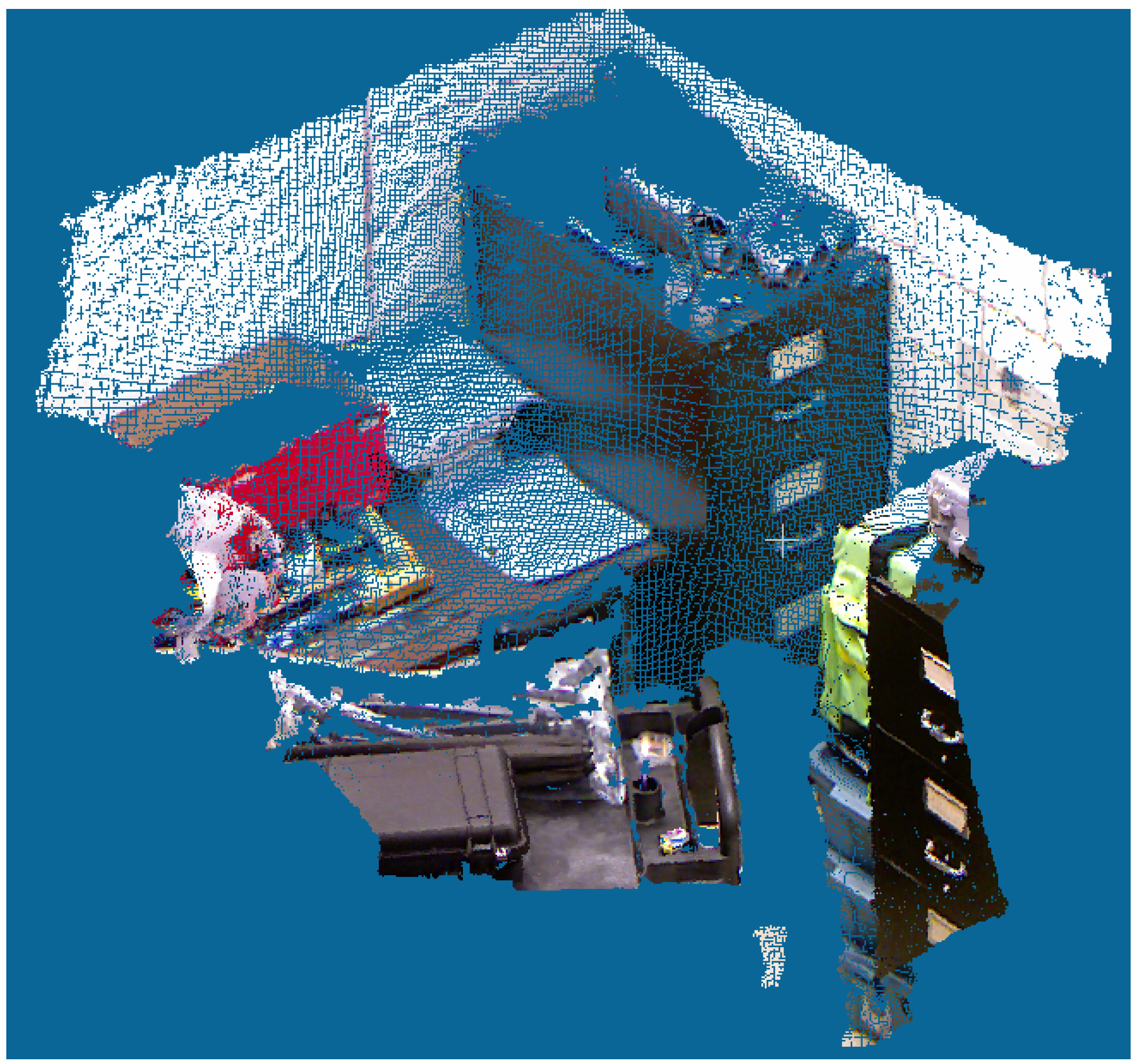
3.3. Point-to-Plane ICP for the Kinect

To compare the proposed ICP algorithm to the widely accepted point-to-plane ICP from Chen and Medioni, the Kinect was mounted on a translation stage while imaging a complex scene between 0.9 m and 2.9 m away (Figure 6). A known translation of 5 cm was then introduced in the depth direction of the Kinect with a standard deviation of 0.05 mm and then a second point cloud was captured. The two point clouds were then registered using the two ICP algorithms. The RMSE of the fit between the two point clouds computed using the point-to-plane distances metric was 7 mm using either algorithm. Also, based on a qualitative analysis of the registered point clouds, no apparent differences between the two methods were identifiable. However, there is a slight difference between the recovered movements of the Kinect. The method by Chen and Medioni [36] underestimated the translation by 1.1 mm and the proposed method underestimated the translation by 0.1 mm. This small improvement comes from the weights assigned to correspondences (based on the triangulation geometry) and a cost function which minimizes the reprojection error of the IR camera and projector pair. Differences of a millimeter may seem insignificant at first, but in the absence of additional information the errors can accumulate rather quickly in a Kinect-only dead-reckoning solution, especially when the Kinect is capturing with a frequency as high as 30 Hz.
Figure 6. Calibrated RGB-D data from Kinect of the scene used for testing iterative closest point (ICP).
Robotics 03 00247 g006
To test the suitability of the devised ICP algorithm for mapping applications when assisted by an Xsens MTi-30 IMU, a sequence of handheld data was captured. This illustrates the mapping abilities when this module is removed from the main trolley platform for exploring inaccessible spaces like stairs before returning to its forced centered position. The Kinect and the MTi-30 were rigidly mounted together with the Kinect logging at 10 Hz and the MTi-30 logging at 100 Hz. A person carried the Kinect and IMU by hand, ascended a flight of stairs, turned around and then descended the same flight of stairs. A total of 315 RGB-D datasets were captured and processed. The final 3D point cloud of the staircase is shown in Figure 7 where the colors are assigned based on the local normals. Considering that the distances travelled was short, the model-to-scene registration scheme was capable of partially handle the loop-closure problem and no apparent misfits can be identified near the bottom of the staircase. For a quantitative accuracy assessment, 20 horizontal and vertical planes were extracted and the overall RMSE from this check plane analysis was 7.0 mm.
Figure 7. Stairs reconstructed using the Kinect and inertial measurement unit (IMU) in a human carried walking sequence.
Robotics 03 00247 g007

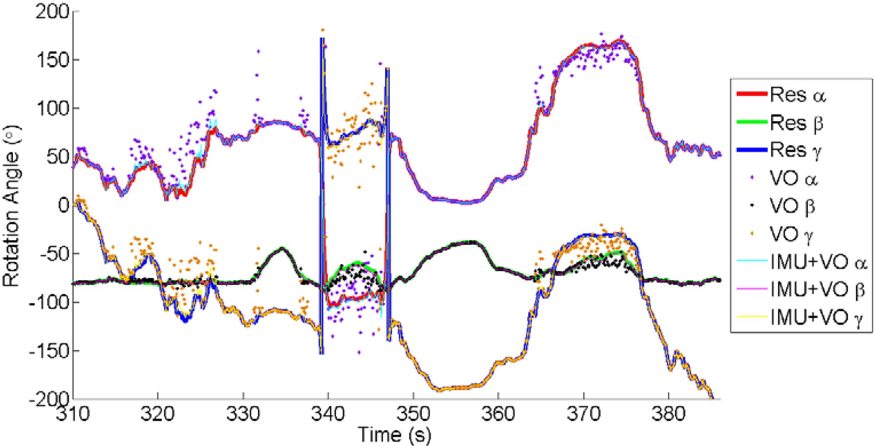
3.4. 2D-to-2D Visual Odometry for Monocular Vision

A checkerboard pattern with known dimensions was imaged with the Kinect’s RGB camera. The Kinect was handheld and waved in front of the checkerboard for approximately 80 s. The reference solution was generated using photogrammetric resection solved in a least-squares adjustment frame-by-frame. This represents the best case scenario in camera navigation where known control points are always visible. VO was performed by solving for the camera’s pose using the mathematical model presented in Equation (10) with the first image held as the reference keyframe the entire time. The camera orientations converted from quaternion to Euler angles are shown in Figure 8. It can be observed that the VO solution follows the reference solution quite closely over certain sections of the plot (e.g., between 350 and 362 s). But in other sections a noticeable difference in their estimation can be observed, with errors reaching as high as 80°. The main cause for such a discrepancy is the intersection geometry. When the pair of images were captured near proximity of each other, the parallax angle is small, this results in a less accurate scene reconstruction, which translates into poor egomotion estimation. In fact, the proposed math model has a singularity when the light rays in the pair of images are all parallel with each other. However, this can easily be identified by checking the disparity of conjugate points. The case when the disparities are all below a threshold actually indicates the camera has not moved significantly, suggesting the possibility of the camera being static, therefore ZUPT was performed. For a MEMS-based IMU, integration of the gyroscope readings alone over a period of approximately 80 s would have introduced a noticeable rotation drift. But as witnessed in Figure 8, the fusion of VO with IMU prevented the estimated orientation from drifting. At the same time the IMU smoothed out the vision-based orientation estimates and provided a better orientation estimate when the uncertainty in VO is high, resulting in a final solution that follows the reference solution quite closely over the full trial. This suggests that VO and gyroscope combined can provide a better orientation estimate than either method alone.
Figure 8. Comparison between various ways of estimating monocular camera rotations. α, β, and γ represents the rotation about the x, y, and z axis, respectively. Res represents the photogrammetric resection solution.
Robotics 03 00247 g008

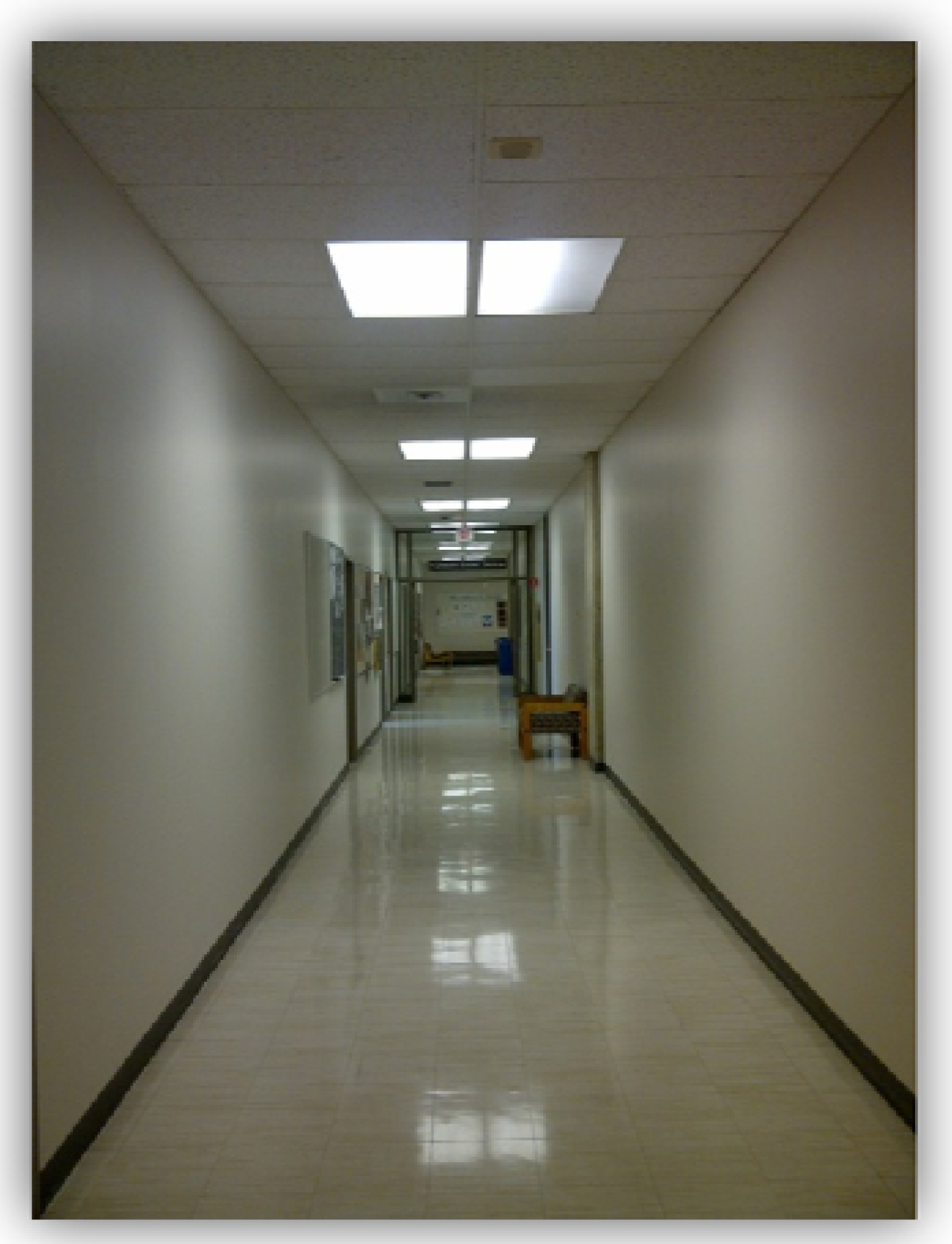
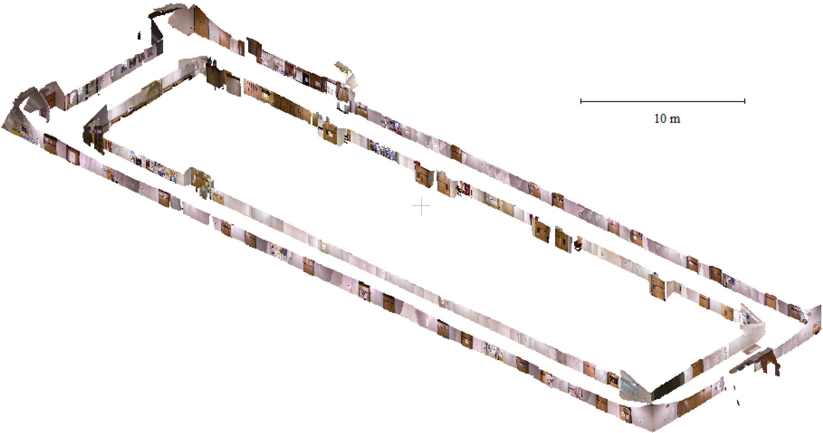
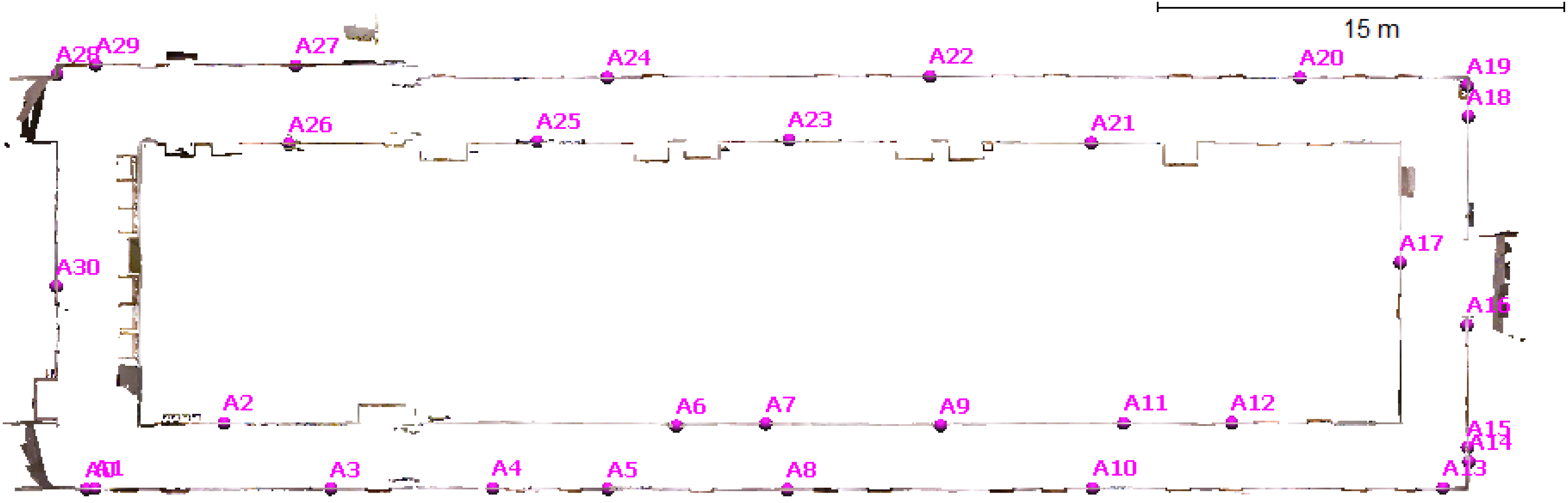
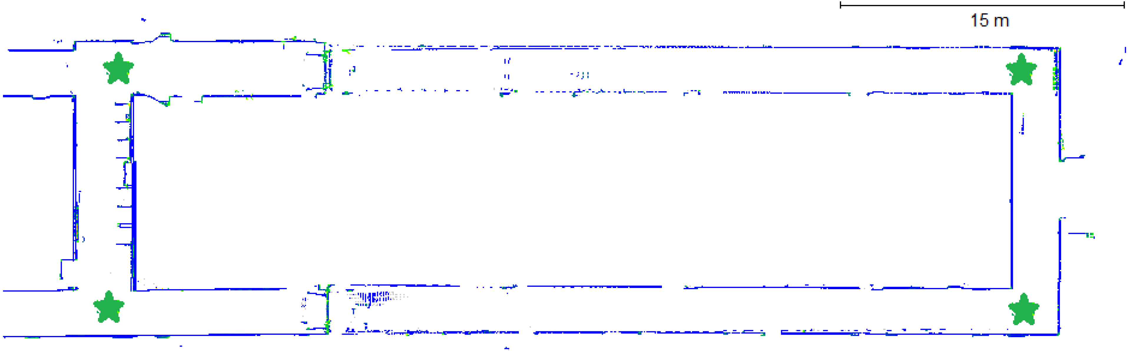
3.5. Scannect Testing at the University of Calgary

The full Scannect system was tested by mapping a floor in the Math Science building located at the University of Calgary, Canada (Figure 9). The hallways are mainly composed of doors (some are recessed), posters, bulletin boards, and white homogenous flat walls. The Scannect travelled 120 m in continuous mode and only stopped at the four corners to capture a 7 minutes scan with the Focus3D S. While in continuous mode, both Kinects were capturing data at 10 Hz while the IMU was logging at 200 Hz. Because the floor was relatively flat, a height constraint was applied. Also, ZUPTS were applied every time sufficiently small movements were detected by the RGB VO and when the Focus3D S was scanning. The total time it took to map the floor in the field was 35 minutes, significantly less than a typical laser scanner only project over such a large area. The processing time for both Kinects with the IMU was about two hours, however it should be stressed that the C++ code implemented has yet to be optimized. The map generated by the Kinect with RGB texture information added for visual appearance is shown in Figure 10. Although only the points measured by the Kinects are shown, these results were generated with the assistance of the Focus3D S. At the beginning a 360° scan was first captured by the scanner and added to the scene. Then the Kinects used this as the scene in the dense 3D matching step. Meanwhile it filled in some occlusions and expands the map until it arrived at the next corner where another laser scan was captured and matched to the scene through the point-to-plane ICP with the IMU predicted pose as the initial alignment. This process was repeated until the floor had been explored (completely mapped).
Throughout the floor, 30 checkpoints were also captured by the Kinects. A top view of the Kinects’ map along with the horizontal distribution of these signalized targets is shown in Figure 11. Due to the limited vertical FOV of the Kinects, all the checkpoints were approximately at the same height. The RMSE in the X, Y, and Z direction was 10.0 cm, 10.8 cm, and 9.0 cm, respectively. This is approximately 0.14% error over the travelled distance. These error estimates only indicates the forward filtering solution and is already similar if not better than the existing methods described in Section 1.3 (i.e., [42,56,57]). After backward smoothing or SBA, the results are expected to improve [41]. Note that the laser scanner only solution shown in Figure 12 (with the green stars indicating the static scan locations) missed a lot of the doorways (in particular the top corridor between targets A26 and A18) but the general shape of the floor is prevalent. This general shape from the laser scans aided the Kinects’ localization and provided some degree of loop-closure. From Figure 11 it can be perceived that the details such as doorways that were missed by the laser scanner were well localized in the same coordinate system by the Kinect. Some misalignments in the scanner data can be observed (e.g., the top corridor), this is likely a result of errors in the initial alignment provided by the Kinect and IMU filter and the accumulated mapping errors.
Figure 9. Image of one of the hallways in the Math Science building at the University of Calgary.
Robotics 03 00247 g009
Figure 10. Oblique view of the Kinect point clouds from the 3D reconstructed scene.
Robotics 03 00247 g010
Figure 11. Top view of the Kinect point clouds from the 3D reconstructed scene. The magenta labels indicate the location of the check points.
Robotics 03 00247 g011
Figure 12. Top view of the laser scanner point clouds from the 3D reconstructed scene with the ceiling and floor removed. The green stars indicate the scan stations.
Robotics 03 00247 g012

4. Conclusions and Future Work

SLAM is a theoretically matured subject with many practical implementation challenges. A few of these challenges were addressed in this paper: the implicit iterative extended Kalman filter was responsible for fusing measurement updates from the Kinect’s RGB and depth stream separately to account for their timing errors and non-linearity of implicit photogrammetry equations; using only the RGB images, a 5-point visual odometry was performed in a tightly-coupled manner while eliminating the need to add or remove states in the filter; a new tightly-coupled ICP method for stereo-vision systems was used for processing the depth maps. The presented Scannect system is the first multi-Kinect mobile mapping system and the first to adopt the continuous stop-and-go design. This system can map an entire building floor efficiently with a Mean Radial Spherical Error of 17 cm. It was capable of navigating in areas with as little features as a single white wall.
In the future, more Kinects will be added to further increase the field of view of the Scannect. For instance, to make the Scannect more flexible and account for sloped floors, a skyward facing Kinect can be added without any modifications to the algorithms and processing pipeline presented in this paper. Newer 3D cameras with a wider field of view (e.g., PMD CamBoard nano) or higher accuracy (e.g., Kinect 2) will be considered. The LiDAR system will be tightly-coupled to allow weighting in the spherical coordinate system. Adding other autonomous non-vision-based sensors such as wheel odometers, magnetometers, and barometers will be beneficial for localization. Other non-holonomic constraints such as leveling updates can also be included if applicable. A more accurate scene representation such as surfels will be adopted [87]. To better handle loop-closures, methods like sparse bundle adjustment will be implemented to improve the global consistency. This was shown to be more accurate than TORO (a graph-based method) when using the Kinect [41]. For real-time online processing and visualization, general-purpose computing on graphics processing units (GPGPU) will be investigated to expedite the filtering process.

Acknowledgments

This research is funded by the Natural Science and Engineering Research Council (NSERC) of Canada, Alberta Innovates, the Canada Foundation for Innovation, and the Killam Trust.

Author Contributions

Jacky C.K. Chow prepared the manuscript; acquired the datasets using the laser scanner, Kinects, and IMU; developed software for manipulating, processing, and integrating data from the sensors; formulated the modified ICP algorithm and 5-point VO algorithm; deciding on the choice of sensors; coming up with the hybrid system design; and testing the Scannect and analyzing its results. Derek D. Lichti provided valuable input to the manuscript. Jeroen D. Hol, Giovanni Bellusci, Henk Luinge assisted in the IMU processing, had valuable insights for the project, and contributed to the writing of this manuscript.

Conflicts of Interest

The authors declare no conflict of interest.

References

  1. Gadeke, T.; Schmid, J.; Zahnlecker, M.; Stork, W.; Muller-Glaser, K. Smartphone pedestrian navigation by foot-IMU sensor fusion. In Proceedings of the 2nd International Conference on Ubiquitous Positioning, Indoor Navigation, and Location Based Service, Helsinki, Finland, 3–4 October 2012; pp. 1–8.
  2. Durrant-Whyte, H.; Bailey, T. Simultaneous localization and mapping: Part I. IEEE Robot. Autom. Mag. 2006, 13, 99–110. [Google Scholar] [CrossRef]
  3. Bailey, T.; Durrant-Whyte, H. Simultaneous localisation and mapping (SLAM): Part II state of the art. IEEE Robot. Autom. Mag. 2006, 13, 108–117. [Google Scholar] [CrossRef]
  4. Huang, A.; Bachrach, A.; Henry, P.; Krainin, M.; Maturana, D.; Fox, D.; Roy, N. Visual odometry and mapping for autonomous flight using an RGB-D camera. In Proceedings of the 15th International Symposium on Robotics Research, Flagstaff, AZ, USA, 28 August–1 September 2011.
  5. He, B.; Yang, K.; Zhao, S.; Wang, Y. Underwater simultaneous localization and mapping based on EKF and point features. In Proceedings of the International Conference on Mechatronics and Automation, Changchun, China, 9–12 August 2009; pp. 4845–4850.
  6. Kuo, B.; Chang, H.; Chen, Y.; Huang, S. A light-and-fast SLAM algorithm for robots in indoor environments using line segment map. J. Robot. 2011. [Google Scholar] [CrossRef]
  7. Newman, P.; Cole, D.; Ho, K. Outdoor SLAM using visual appearance and laser ranging. In Proceedings of the IEEE International Conference on Robotics and Automation, Orlando, FL, USA, 15–19 May 2006; pp. 1180–1187.
  8. Georgiev, A.; Allen, P. Localization methods for a mobile robot in urban environments. IEEE Trans. Robot. 2004, 20, 851–864. [Google Scholar] [CrossRef]
  9. Kümmerle, R.; Steder, B.; Dornhege, C.; Kleiner, A.; Grisetti, G.; Burgard, W. Large scale graph-based SLAM using aerial images as prior information. J. Auton. Robots 2011, 30, 25–39. [Google Scholar] [CrossRef]
  10. Vosselman, G.; Maas, H.-G. Airborne and Terrestrial Laser Scanning; Whittles Publishing: Caithness, UK, 2010. [Google Scholar]
  11. Nüchter, A. Parallelization of scan matching for robotic 3D mapping. In Proceedings of the 3rd European Conference on Mobile Robots, Freiburg, Germany, 19–21 September 2007.
  12. Lin, Y.; Hyyppä, J.; Kukko, A. Stop-and-go mode: Sensor manipulation as essential as sensor development in terrestrial laser scanning. Sensors 2013, 13, 8140–8154. [Google Scholar] [CrossRef]
  13. Ferris, B.; Fox, D.; Lawrence, N. WiFi-SLAM using Gaussian process latent variable models. In Proceedings of the 20th International Joint Conference on Artificial Intelligence, Hyderabad, India, 6–12 January 2007; pp. 2480–2485.
  14. Des Bouvrie, B. Improving rgbd indoor mapping with imu data. Master’s Thesis, Delft University of Technology, Delft, The Netherlands, 2011. [Google Scholar]
  15. Strasdat, H.; Montiel, J.; Davison, A. Real-time monocular SLAM: Why filter? In Proceedings of the IEEE International Conference on Robotics and Automation, Anchorage, AK, 3–7 May 2010; pp. 2657–2664.
  16. Tomono, M. Robust 3D SLAM with a stereo camera based on an edge-point ICP algorithm. In Proceedings of the IEEE International Conference on Robotics and Automation, Kobe, Japan, 12–17 May 2009; pp. 4306–4311.
  17. Borrmann, D.; Elseberg, J.; Lingemann, K.; Nüchter, A.; Hertzberg, J. Globally consistent 3D mapping with scan matching. Robot. Auton. Syst. 2008, 56, 130–142. [Google Scholar] [CrossRef]
  18. May, S.; Fuchs, S.; Droeschel, D.; Holz, D.; Nüchter, A. Robust 3D-mapping with time-of-flight cameras. In Proceedings of the IEEE/RSJ International Conference on Intelligent Robots and Systems, St. Louis, MO, USA, 10–15 October 2009; pp. 1673–1678.
  19. Siegwart, R.; Nourbakhsh, I.; Scaramuzza, D. Introduction to Autonomous Mobile Robots, 2nd ed.; The MIT Press: Cambridge, MA, USA, 2011. [Google Scholar]
  20. Luhmann, T.; Robson, S.; Kyle, S.; Harley, I. Close Range Photogrammetry: Principles, Techniques and Applications; Whittles Publishing: Caithness, UK, 2006. [Google Scholar]
  21. Mishra, R.; Zhang, Y. A review of optical imagery and airborne LiDAR data registration methods. Open Remote Sens. J. 2012, 5, 54–63. [Google Scholar] [CrossRef]
  22. Kurz, T.; Buckley, S.; Schneider, D.; Sima, A.; Howell, J. Ground-based hyperspectral and lidar scanning: A complementary method for geoscience research. In Proceedings of the International Association for Mathematical Geosciences, Salzburg, Austria, 5–9 September 2011.
  23. Han, J.; Shao, L.; Xu, D.; Shotton, J. Enhanced computer vision with Microsoft Kinect sensor: A review. IEEE Trans. Cybern. 2013, 43, 1318–1334. [Google Scholar] [CrossRef]
  24. Zug, S.; Penzlin, F.; Dietrich, A.; Nguyen, T.; Albert, S. Are laser scanners replaceable by Kinect sensors in robotic applications? In Proceedings of the IEEE International Symposium on Robotic and Sensors Environments (ROSE), Magdeburg, Germany, 16–18 November 2012; pp. 144–149.
  25. Meister, S.; Kohli, P.; Izadi, S.; Hämmerle, M.; Rother, C.; Kondermann, D. When can we use KinectFusion for ground truth acquisition? In Proceedings of the IEEE/RSJ International Conference on Intelligent Robots and Systems, Workshop on Color-Depth Camera Fusion in Robotics, Vilamoura, Algarve, Portugal, 7–11 October 2012.
  26. Smisek, J.; Jancosek, M.; Pajdla, T. 3D with kinect. In Proceedings of the Consumer Depth Cameras for Computer Vision, Barcelona, Spain, 12 November 2011.
  27. Stoyanov, T.; Louloudi, A.; Andreasson, H.; Lilienthal, A. Comparative evaluation of range sensor accuracy for indoor environments. In Proceedings of the European Conference on Mobile Robots, Örebro, Sweden, 7–9 September 2011; pp. 19–24.
  28. Chow, J.; Ang, K.; Lichti, D.; Teskey, W. Performance analysis of a low-cost triangulation-based 3D camera: Microsoft Kinect system. In Proceedings of the International Society of Photogrammetry and Remote Sensing Congress, Melbourne, Australia, 25 August–1 September 2012.
  29. Renaudin, V.; Yalak, O.; Tomé, P.; Merminod, B. Indoor navigation of emergency agents. Eur. J. Navig. 2007, 5, 36–45. [Google Scholar]
  30. Ghilani, C.; Wolf, P. Elementary Surveying: An Introduction to Geomatics, 12th ed.; Prentice Hall: Upper Saddle River, NJ, USA, 2008. [Google Scholar]
  31. Grisetti, G.; Stachniss, C.; Burgard, W. Improving grid-based SLAM with with Rao-Blackwellized particle filters by adaptive proposals and selective resampling. In Proceedings of the IEEE International Conference on Robotics and Automation, Barcelona, Spain, 18–22 April 2005; pp. 2432–2437.
  32. Gustafsson, F. Statistical Sensor Fusion, 2nd ed.; Studentlitteratur AB: Lund, Sweden, 2010. [Google Scholar]
  33. Scaramuzza, D.; Fraundorfer, F. Visual odometry part I: The first 30 years and fundamentals. IEEE Robot. Autom. Mag. 2011, 18, 80–92. [Google Scholar]
  34. Besl, P.; McKay, N. A method for registration of 3D shapes. IEEE Trans. Pattern Anal. Mach. Intell. 1992, 14, 239–256. [Google Scholar] [CrossRef]
  35. Horn, B. Closed-form solution of absolute orientation using unit quaternions. J. Opt. Soc. Am. 1987, 4, 629–642. [Google Scholar] [CrossRef]
  36. Chen, Y.; Medioni, G. Object modelling by registration of multiple range images. Image Vis. Comput. 1992, 10, 145–155. [Google Scholar] [CrossRef]
  37. Rusinkiewicz, S.; Levoy, M. Efficient variants of the ICP algorithm. In Proceedings of the 3rd International Conference on 3-D Digital Imagining and Modeling, Quebec, QC, Canada, 28 May–1 June 2001; pp. 145–152.
  38. Klein, G.; Murray, D. Parallel tracking and mapping for small AR workspaces. In Proceedings of the 6th IEEE and ACM International Symposium on Mixed and Augmented Reality, Nara, Japan, 13–16 November 2007; pp. 225–234.
  39. Nützi, G.; Weiss, S.; Scaramuzza, D.; Siegwart, R. Fusion of IMU and vision for absolute scale estimation in monocular SLAM. J. Intell. Robot. Syst. 2011, 61, 287–299. [Google Scholar] [CrossRef]
  40. Scherer, S.; Dube, D.; Zell, A. Using depth in visual simultanesous localisation and mapping. In Proceedings of the IEEE International Conference on Robotics and Automation, St. Paul, MN, USA, 14–18 May 2012.
  41. Henry, P.; Krainin, M.; Herbst, E.; Ren, X.; Fox, D. RGB-D mapping: Using Kinect-style depth cameras for dense 3D modeling of indoor environments. Int. J. Robot. Res. 2012, 31, 647–663. [Google Scholar] [CrossRef]
  42. Henry, P.; Krainin, M.; Herbst, E.; Ren, X.; Fox, D. RGB-D mapping: Using depth cameras for dense 3d modeling of indoor environments. In Proceedings of the RGB-D: Advanced Reasoning with Depth Cameras in Conjunction with Robotics Science and Systems, Zaragoza, Spain, 27 June 2010.
  43. Johnson, A.; Kang, S. Registration and integration of textured 3D data. Image Vis. Comput. 1999, 17, 135–147. [Google Scholar] [CrossRef]
  44. Izadi, S.; Kim, D.; Hilliges, O.; Molyneaux, D.; Newcombe, R.; Kohli, P.; Shotton, J.; Hodges, S.; Freeman, D.; Davison, A.; et al. KinectFusion: Real-time 3D reconstruction and interaction using a moving depth camera. In Proceedings of the 24th ACM Symposium on User Interface Software and Technology, Santa Barbara, CA, USA, 16–19 October 2011; pp. 559–568.
  45. Curless, B.; Levoy, M. A volumetric method for building complex odels from range images. In Proceedings of the 23rd Annual Conference on Computer Graphics and Interactive Techniques—SIGGRAPH, New York, NY, USA, 4–9 August 1996; pp. 303–312.
  46. Whelan, T.; McDonald, J.; Kaess, M.; Fallon, M.; Johannsson, H.; Leonard, J. Kintinuous: Spatially extended KinectFusion. In Proceedings of the 3rd RSS Workshop on RGB-D: Advanced Reasoning with Depth Cameras, Sydney, Australia, 9–10 July 2012.
  47. Whelan, T.; Johannsson, H.; Kaess, M.; Leonard, J.; McDonald, J. Robust real-time visual odometry for dense RGB-D mapping. In Proceedings of the IEEE International Conference on Robotics and Automation, Karlsruhe, Germany, 6–10 May 2013; pp. 5724–5731.
  48. Whelan, T.; Kaess, M.; Leonard, J.; McDonald, J. Deformation-based loop closure for large scale dense RGB-D SLAM. In Proceedings of the IEEE/RSJ International Conference on Intelligent Robots and Systems, Tokyo, Japan, 3–8 November 2013.
  49. Keller, M.; Lefloch, D.; Lambers, M.; Izadi, S.; Weyrich, T.; Kolb, A. Real-time 3D reconstruction in dynamic scenes using point-based fusion. In Proceedings of the International Conference on 3D Vision, Seattle, WA, USA, 29 June–1 July 2013; pp. 1–8.
  50. Khoshelham, K.; Dos Santos, D.; Vosselman, G. Generation and weighting of 3D point correspondences for improved registration of RGB-D data. In Proceedings of the ISPRS Annals of the Photogrammetry and Remote Sensing and Spatial Information Sciences, Antalya, Turkey, 11–13 November 2013; Volume II-5/W2.
  51. Leutenegger, S.; Furgale, P.; Rabaud, V.; Chli, M.; Konolige, K.; Siegwart, R. Keyframe-based visual-inertial SLAM using nonlinear optimization. In Proceedings of the Robotics: Science and Systems, Berlin, Germany, 24–28 June 2013.
  52. Li, L.; Cheng, E.; Burnett, I. An iterated extended Kalman filter for 3D mapping via Kinect camera. In Proceedings of the IEEE International Conference on Acoustics, Speech and Signal Processing, Vancouver, Canada, 26–31 May 2013; pp. 1773–1777.
  53. Aghili, F.; Kuryllo, M.; Okouneva, G.; McTavish, D. Robust pose estimation of moving objects using laser camera data for autonomous rendezvous and docking. In Proceedings of the International Society of Photogrammetry and Remote Sensing Archives, Paris, France, 1–3 September 2009; Volume XXXVIII-3/W8, pp. 253–258.
  54. Hervier, T.; Bonnabel, S.; Goulette, F. Accurate 3D maps from depth images and motion sensors via nonlinear Kalman filtering. In Proceedings of the IEEE/RSJ International Conference on Intelligent Robots and Systems, Vilamoura, Portugal, 7–12 October 2012; pp. 5291–5297.
  55. Kottas, D.; Roumeliotis, S. Exploiting urban scenes for vision-aided inertial navigation. In Proceedings of the Robotics: Science and Systems, Berlin, Germany, 24–28 June 2013.
  56. Li, M.; Kim, B.; Mourikis, A. Real-time motion tracking on a cellphone using inertial sensing and a rolling shutter camera. In Proceedings of the IEEE International Conference on Robotics and Automation, Karlsruhe, Germany, 6–10 May 2013.
  57. Burens, A.; Grussenmeyer, P.; Guillemin, S.; Carozza, L.; Lévêque, F.; Mathé, V. Methodological developments in 3D scanning and modelling of archaeological French heritage site: The bronze age painted cave of Les Fraux, Dordogne (France). In Proceedings of the International Archives of the Photogrammetry, Remote Sensing and Spatial Information Sciences, Strasbourg, France, 2–6 September 2013; Volume XL-5/W2, pp. 131–135.
  58. Chiabrando, F.; Spanò, A. Point clouds generation using TLS and dense-matching techniques. A test on approachable accuracies of different tools. In Proceedings of the ISPRS Annals of the Photogrammetry, Remote Sensing and Spatial Information Sciences, Strasbourg, France, 2–6 September 2013; Volume II-5/W1, pp. 67–72.
  59. Khoshelham, K.; Oude Elberink, S. Accuracy and resolution of kinect depth data for indoor mapping applications. Sensors 2012, 12, 1437–1454. [Google Scholar] [CrossRef]
  60. Dal Mutto, C.; Zanuttigh, P.; Cortelazzo, G. Time-of-Flight Cameras and Microsoft Kinect; Springer: New York, NY, USA, 2013. [Google Scholar]
  61. Kainz, B.; Hauswiesner, S.; Reitmayr, G.; Steinberger, M.; Grasset, R.; Gruber, L.; Veas, E.; Kalkofen, D.; Seichter, H.; Schmalstieg, D. OmniKinect: Real-time dense volumetric data acquisition and applications. In Proceedings of the 18th ACM Symposium on Virtual Reality Software and Technology, Toronto, ON, Canada, 10–12 December 2012; pp. 25–32.
  62. Butler, A.; Izadi, S.; Hilliges, O.; Molyneaux, D.; Hodges, S.; Kim, D. Shake and sense: Reducing interference for overlapping structured light depth cameras. In Proceedings of the SIGCHI Conference on Human Factors in Computing Systems, Austin, TX, USA, 5–10 May 2012; pp. 1933–1936.
  63. Aggarwal, P.; Syed, Z.; Noureldin, A.; El-Sheimy, N. MEMS-Based Integrated Navigation; Artech House: Norwood, MA, USA, 2010. [Google Scholar]
  64. Herrera, D.; Kannala, J.; Heikkilä, J. Joint depth and color camera calibration with distortion correction. IEEE Trans. Pattern Anal. Mach. Intell. 2012, 34, 2058–2064. [Google Scholar] [CrossRef]
  65. Chow, J.; Lichti, D. Photogrammetric bundle adjustment with self-calibration of the PrimeSense 3D camera technology: Microsoft Kinect. IEEE Access 2013, 1, 465–474. [Google Scholar] [CrossRef]
  66. Lichti, D. Error modelling, calibration and analysis of an AM-CW terrestrial laser scanner system. ISPRS J. Photogramm. Remote Sens. 2007, 61, 307–324. [Google Scholar]
  67. Reshetyuk, Y. A unified approach to self-calibration of terrestrial laser scanners. ISPRS J. Photogramm. Remote Sens. 2010, 65, 445–456. [Google Scholar]
  68. Chow, J.; Lichti, D.; Glennie, C.; Hartzell, P. Improvements to and comparison of static terrestrial LiDAR self-calibration methods. Sensors 2013, 13, 7224–7249. [Google Scholar]
  69. Chow, J.; Lichti, D.; Teskey, W. Accuracy assessment of the Faro Focus3D and Leica HDS6100 panoramic type terrestrial laser scanner through point-based and plane-based user self-calibration. In Proceedings of the FIG Working Week 2012: Knowing to Manage the Territory, Protect the Environment, Evaluate the Cultural Heritage, Rome, Italy, 6–10 May 2012.
  70. Al-Manasir, K.; Fraser, C. Registration of terrestrial laser scanner data using imagery. Photogramm. Rec. 2006, 21, 255–268. [Google Scholar] [CrossRef]
  71. Lobo, J.; Dias, J. Relative pose calibration vetween visual and inertial sensors. Int. J. Robot. Res. 2007, 26, 561–575. [Google Scholar] [CrossRef]
  72. Hol, J.; Schön, T.; Gustafsson, F. Modeling and calibration of inertial and vision sensors. Int. J. Robot. Res. 2009, 29, 231–244. [Google Scholar]
  73. Mirzaei, F.; Roumeliotis, S. A Kalman filter-based algorithm for IMU-camera calibration: Observability analysis and performance evaluation. IEEE Trans. Robot. 2008, 24, 1143–1156. [Google Scholar] [CrossRef]
  74. Titterton, D.; Weston, J. Strapdown Inertial Navigation Technology; IEE Radar, Sonar, Navigation and Avionics Series; Peter Peregrinus Ltd.: Stevenage, UK, 1997. [Google Scholar]
  75. Gelb, A. Applied Optimal Estimation; The MIT Press: Cambridge, MA, USA, 1974. [Google Scholar]
  76. Steffen, R.; Beder, C. Recursive estimation with implicit constraints. In Proceedings of the 29th DAGM Conference on Pattern Recognition, Heidelberg, Germany, 12–14 September 2007; pp. 194–203.
  77. Steffen, R. A robust iterative Kalman filter based on implicit measurement equations. Photogramm. Fernerkund. Geoinf. 2013, 2013, 323–332. [Google Scholar] [CrossRef]
  78. OpenNI Programmer’s Guide. OpenNI 2.0 API. Available online: http://www.openni.org/openni-programmers-guide/ (accessed on 16 December 2013).
  79. Muja, M.; Lowe, D. Fast approximate nearest neighbors with automatic algorithm configuration. In Proceedings of the International Conference on Computer Vision Theory and Applications (VISAPP’09), Lisboa, Portugal, 5–9 February 2009; pp. 331–340.
  80. Luck, J.; Little, C.; Hoff, W. Registration of range data using a hybrid simulated annealing and iterative closest point algorithm. In Proceedings of the IEEE International Conference on Robotics and Automation, San Francisco, CA, USA, 24–28 April 2000; pp. 3739–3733.
  81. Bradski, G.; Kaehler, A. Learning OpenCV; O’Reilly Media: Sabastopol, CA, USA, 2008. [Google Scholar]
  82. Zhong, Y. Intrinsic shape signatures: A shape descriptor for 3D object recognition. In Proceedings of the IEEE 12th International Conference on Computer Vision, Kyoto, Japan, 29 September–2 October 2009; pp. 689–696.
  83. Filipe, S.; Alexandre, L. A comparative Evaluation of 3D keypoint detectors. In Proceedings of the 9th Conference on Telecommunications, Castelo Branco, Portugal, 8–10 May 2013; pp. 145–148.
  84. Tombari, F.; Salti, S.; Di Stefano, L. A combined texture-shape descriptor for enhanced 3D feature matching. In Proceedings of the 18th IEEE International Conference on Image Processing, Brussels, Belgium, 11–14 September 2011; pp. 809–812.
  85. Fraundorfer, F.; Scaramuzza, D. Visual odometry part II: Matching, robustness, optimization, and applications. IEEE Robot. Autom. Mag. 2012, 19, 78–90. [Google Scholar] [CrossRef] [Green Version]
  86. Chow, J.; Ebeling, A.; Teskey, W. Point-based and plane-based deformation monitoring of indoor environments using terrestrial laser scanners. J. Appl. Geod. 2012, 6, 193–202. [Google Scholar]
  87. Pfister, H.; Zwicker, M.; van Baar, J.; Gross, M. Surfels: Surface elements as rendering primitives. In Proceedings of the 27th Annual Conference on Computer Graphics and Interactive Techniques, New Orleans, LA, USA, 23–28 July 2000; pp. 335–342.

