1. Introduction
This paper presents a procedure and some experimental results concerning the auto-calibration of the kinematic parameters of a tracked vehicle, developed for humanitarian demining operations. The vehicle is aimed to bring metal detectors, ground penetrating radars and intelligent probes to discover the presence of buried mines, along with other tools to disarm or detonate them. It is estimated that around 100 million landmines are still present as the result of previous conflicts in more than 84 countries. Classical manual demining operations are very slow and dangerous and need the help of technology. The European Commission (EC) funded project TIRAMISU is developing several tools to speed-up demining operations [
1,
2]. Robots can represent a useful technology for humanitarian demining, allowing human workers to stay at a safe distance during the operations [
3,
4].
Localization is of paramount importance in this and many other robotic applications, in particular when autonomous operations are required. Outdoor mobile robots locate their positions by using GNSS (global navigation satellite systems) such as GPS, which nowadays can reach centimeter-level of accuracy. However in the presence of obstacles, such as big rocks, buildings, or vegetation, the satellite signal can be obstructed and this precision could quickly degrade. In these cases the adoption of relative positioning systems such as odometry, using encoders or Inertial Measurement Units (IMU), can greatly help to localize the robot.
Odometry is mainly based on the assumption that measures of wheel movements can be converted into measures of the robot motion using the kinematic model of the vehicle. This assumption is only of restricted value, because there are a number of factors bringing inaccuracies in the odometry. The main error sources are: wheels slipping, uncertainty in the kinematic parameters (wheel radii and wheelbase), misalignment of the wheels and finite encoder resolution and sampling frequency.
The errors caused by kinematic parameters uncertainty could be reduced if a good calibration is performed. However the errors caused by the wheels slipping cannot be estimated by the encoders and hence cannot be compensated. In particular, for a skid steering robot, during a rotation the estimation of the orientation performed solely by odometry can result in very significant errors. In this case, the adoption of an inertial measurement unit together with a magnetometer can give the measurement of the absolute orientation of the robot. However, the magnetometer should also be calibrated, especially as regard its offset, which for an electric vehicle full of metal parts and magnets, can assume significant variations.
Calibration is essentially the problem of estimating the parameters of the robot model from sensor measures. Several papers in the past have addressed the problem of self-calibration of the kinematic parameters using a wide variety of algorithms and sensors. For example in [
5] an Extended Kalman Filter is adopted to perform the calibration of the parameters of a six-wheel skid steering robot adopted for volcanic explorations. The calibration of the odometric parameters, together with the extrinsic pose estimation of an exteroceptive sensor, is formulated as a maximum-likelihood problem in [
6]. A different approach is presented in [
7], where the calibration is obtained as the solution of an optimization problem with a statistical method. In [
8] an EKF is adopted for odometry calibration of a differential drive robot using the data collected from a floor color sensor. The redundancy of the sensor outputs is adopted to perform the automatic calibration on a multisensor system in [
9], while in [
10] the observable filter is introduced and used together with an augmented Kalman filter for the estimation of the non-systematic odometry error for a mobile robot. In [
11,
12] an EKF is used to estimate wheel slip and “virtual” velocity of a skid-steered mobile robot. An approach to estimate the odometry calibration parameters while performing SLAM is presented in [
13] by using an expectation maximization algorithm, while [
14] extends the graph-based formulation of the SLAM problem to handle the calibration parameters.
However in all these papers the estimation of the magnetometer offset is not considered.
This paper, after a short introduction on the considered platform and sensors, will describe the localization and calibration procedure for the kinematic and for the magnetometer offset and will show some examples of experimental results.
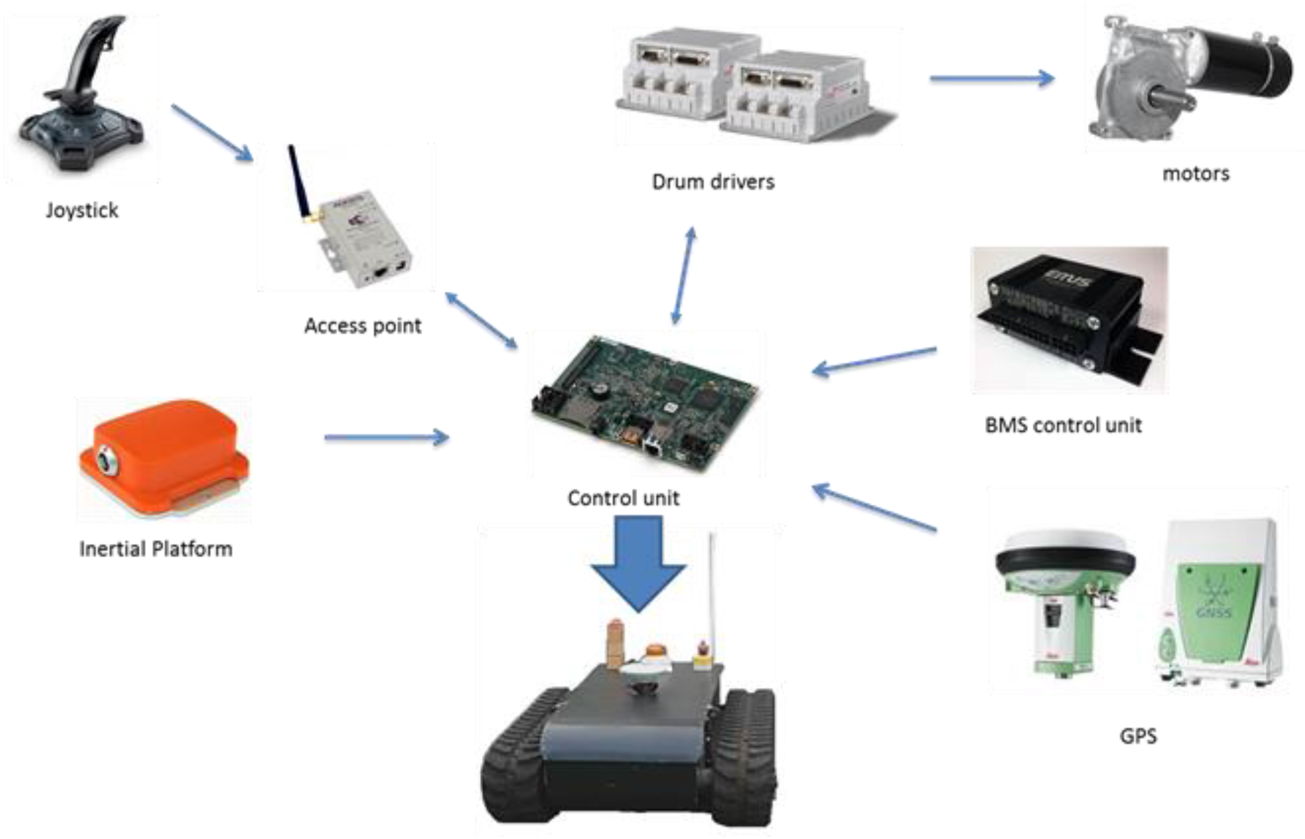
2. The Considered Tracked Platform
The mobile robot used in this work is shown in
Figure 1. This is a tracked robot, in differential drive configuration. Through the tracks, the motion is transmitted from front actuated wheels to the back passive ones. A DC brushed motor actuates each front wheel, which, using the differential configuration, can run with different velocities, in order to control the robot direction.
From the structural point of view, the robot has a central compartment, with dimensions 99.1 cm × 48.5 cm × 28.5 cm. Each track has a width of 18 cm and the distance between the two tracks measures b = 70 cm. The diameter of the actuated wheels is equal to D = 0.16 cm.
Inside the central compartment, as it is shown in
Figure 2, there are:
The embedded robot controller based on the Single Board RIO 9626 (National Instruments).
LiFePO4 battery: eight cells 110 Ah in series.
Battery control unit.
Two DC brushed motors capable to supply a maximum power of 800 W each and to reach speeds of 2800 RPM without load. Each motor is equipped with a gear reducer having a speed reduction ratio of 1/32.
Two digital drives of the series DRUM and produced by Elmo Motion Control, for the motor drive.
Two encoders by Kubler of 1024ppr, placed on each rotor axis of the motors to perform the speed closed loop control.
Four voltage regulators to give the correct power to all the on board devices, including the government units and the sensors.
In regard to other sensors, there is a “Leica gs10” Real Time Kinematics (RTK) Differential GPS (DGPS) system, a SICK LMS200 laser scanner and an Xsense MTI Attitude and Heading Reference System (AHRS), which includes an inertial platform and a triaxial magnetometer. This sensor gives directly the estimation of the attitude and heading of the robot. For the implementation of remotely radio-controlled algorithms, a digital joystick was used for sending linear and angular velocity references, thanks the use of a WI-FI connection, using a wireless Access Point by ACKSYS.
3. Auto-Calibration Methodology
An Extended Kalman Filter (EKF) algorithm is used to fuse the DGPS, encoder and AHRS data, in order to calculate the robot position and direction and to estimate the robot model parameters.
As it was mentioned in the introduction, the calibration of the robot parameters is periodically required. This can be achieved by fusing model data and internal measurements from the encoders, with external sensorial data obtained from the GPS and the AHRS platform.
3.1. Robot Kinematic Model
The robot is characterized by a position
and an orientation
on a horizontal plane:
where
and
are respectively the linear and angular speed of the robot. The discretized model is simply calculated as it follows:
where
T represents the sampling time.
Two optical encoders are used for evaluating the angular displacement of the robot wheels. Then
and
are calculated by the following equations:
where:
and , are respectively the displacement of the right and left wheels, during the interval ;
and represent the radii of the right and left wheels, including track width;
L is the wheelbase, i.e., the distance between left and right tracks.
Combining the last equations, the mathematical model of the robot becomes:
The EKF localization algorithm, using odometry measures, computes at high frequency the
expected position and
orientation of the robot, and the
update phase corrects these estimations at a lower frequency using the GPS and AHRS platform measures [
15]. The odometry parameters are considered as state variables in the EKF. In particular once defined the
state vector:
The mathematical model becomes:
The inputs of the kinematic model are the encoder measures:
while the output vector is represented by the robot position:
where
H is the following matrix:
The kinematic model, so, can be simply written as:
where
w(k) is the process noise which is assumed to be drawn from a zero mean multivariate normal distribution with covariance
Cw while
v(k) is the observation noise which is assumed to be zero mean Gaussian white noise with covariance
Cv.
3.2. Self-Calibrating Extended Kalman Filter (SC EKF)
3.2.1. Predictive Phase
The predictive phase of the EKF algorithm, calculates the
predicted state
and the predicted covariance matrix
where:
is the covariance matrix and represents the uncertainty of the estimated state;
is the covariance matrix of the input noise;
and are the Jacobians of the system.
3.2.2. Update Phase
The GPS and AHRS platform measurements, which represent the external sensorial data, are read asynchronously with respect to the odometry ones: the encoders’ measures are available at higher frequencies.
When a new external sensorial measurement is not available, the update phase is very simple: the state and the covariance matrix are obtained directly from the predicted state vector and the covariance matrix, while, if a new sensorial measurement is available, the Kalman Gain Matrix is calculated in order to update the results. Since we have two kinds of external sensorial measures, it is better to realize two update phases in series.
AHRS Update Phase
where
is the measure covariance matrix, obtained directly from the AHRS platform data:
With , representing the yaw uncertainty of the MTI AHRS sensor.
The measurement vector is also obtained directly from the AHRS platform measures:
The predicted measurement vector is:
The measurement vector is compared to the predicted measurement vector in order to obtain the estimated state
, using the Kalman Gain Matrix:
and the state covariance matrix is evaluated as follows:
GPS Update Phase
A similar procedure is performed for this phase, taking into account that in the previous case, only a measurement for each cycle was done. Now with the GPS data, two measurements for cycle are available, so great attention should be given to the matrices dimensions.
Starting from the state vector and the covariance matrix, evaluated in the previous update phase:
where
is the measurement covariance matrix, obtained directly from the GPS data:
Observe that value changes, according to the quality of the GPS signal.
The measurement vector is obtained directly from the GPS measures:
The predicted measurement vector is:
The measurement vector is compared to the predicted measurement vector in order to obtain the estimated state
, using the Kalman Gain Matrix:
and the state covariance matrix is evaluated as follows:
Obviously, if the AHRS measurements are not available, the AHRS update phase will not be executed. Then GPS update will work with state vector and covariance matrix evaluated during the prediction phase with:
Similarly, if GPS measurements are not available, only the AHRS update phase will be executed. In this last case:
3.3. EKF with Offset Estimation
In this work, EKF was also used for another important aspect. Indeed, during experimental robot motions, it was possible to see a significant magnetic disturbance effect of building structures and robot structures on the magnetometer in the AHRS. This negative effect does not allow reaching very good results in terms of localization, because the acquired orientation data of the robot are affected by large errors. This means that the path reconstruction of the Kalman filter is not sufficient to predict the exact position of the robot and to localize its correct position, in case of GPS signal loss or low precision of GPS position coordinates.
This is why it was necessary to compensate the value of this disturbance, which can be seen as an offset, in order to improve EKF performances. An initial calibration was not sufficient, since it was experimentally observed that this offset value is not constant during long trajectories.
Another state variable, called “
Ofs”, was added into the model:
In this way, the mathematical model becomes:
Now the model consists in seven equations, so also the Jacobian matrices and all the dimensions of the matrices of the filter also change.
The measurement vector is obtained again directly from the AHRS platform measures according to Equation (15), however the predicted measurement vector is now modified into:
Since it now takes into account the presence of the offset and in this way it affects the angle estimation.
4. Experimental Results
The previous equations have been implemented in the adopted control board SbRIO 9626 by National Instruments. The board was programmed using the LabViewTM programming language.
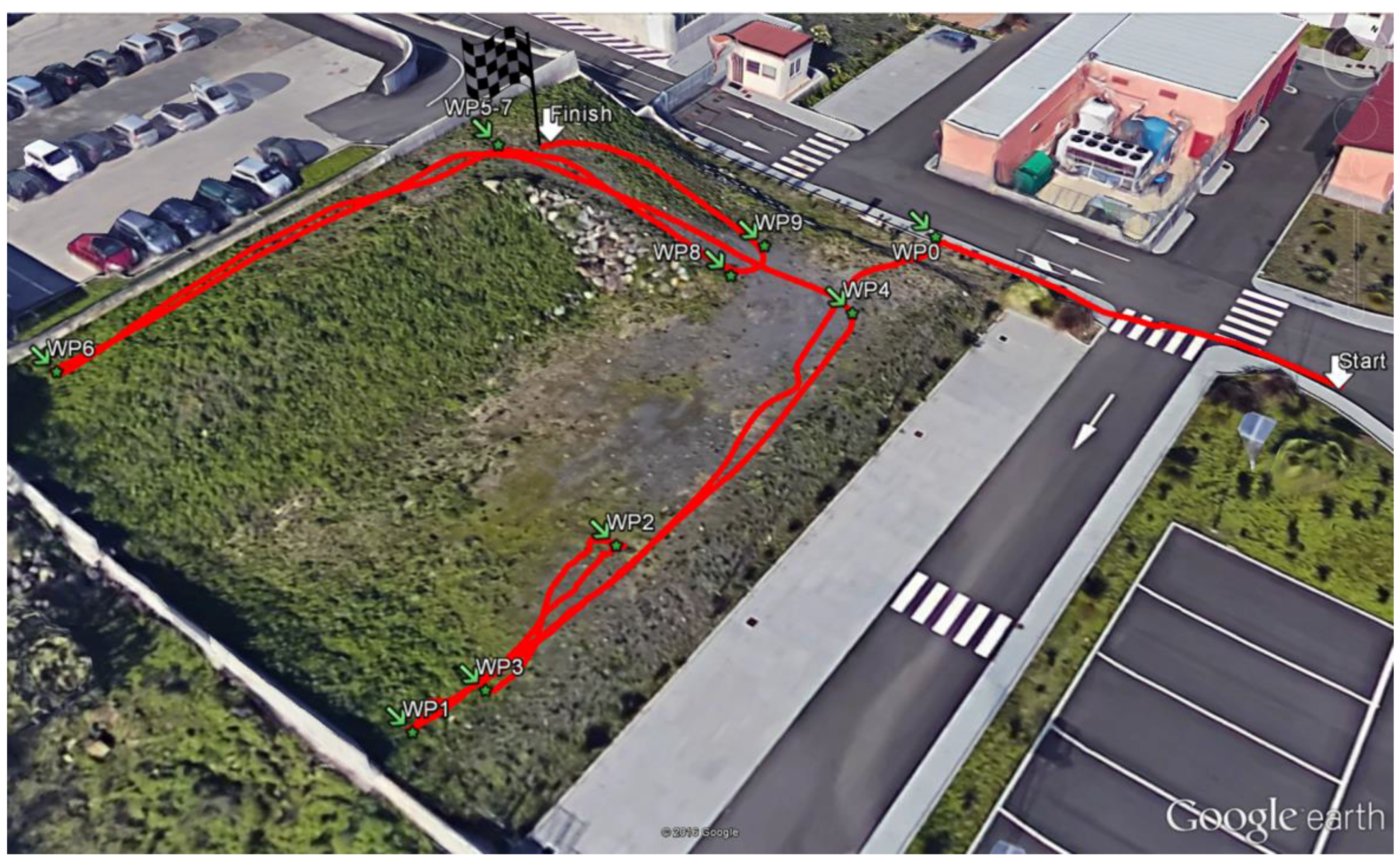
Various tests in different conditions have been performed. In the first two experiments two different trajectories, a circular path and a rectangular path, have been considered for each condition. Finally for the last trial a general-shape trajectory was also considered, reporting also more results in term of parameters estimation.
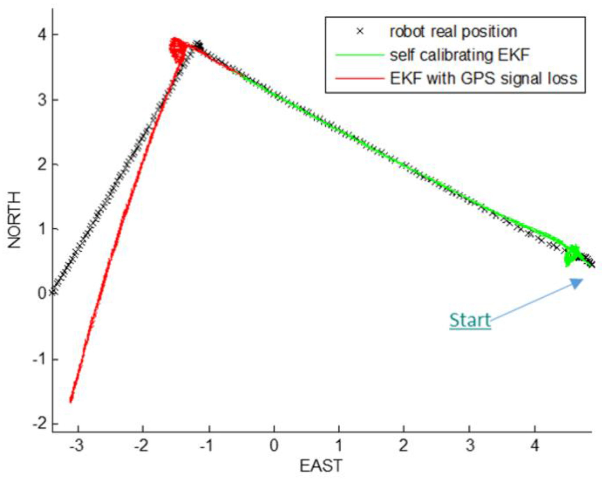
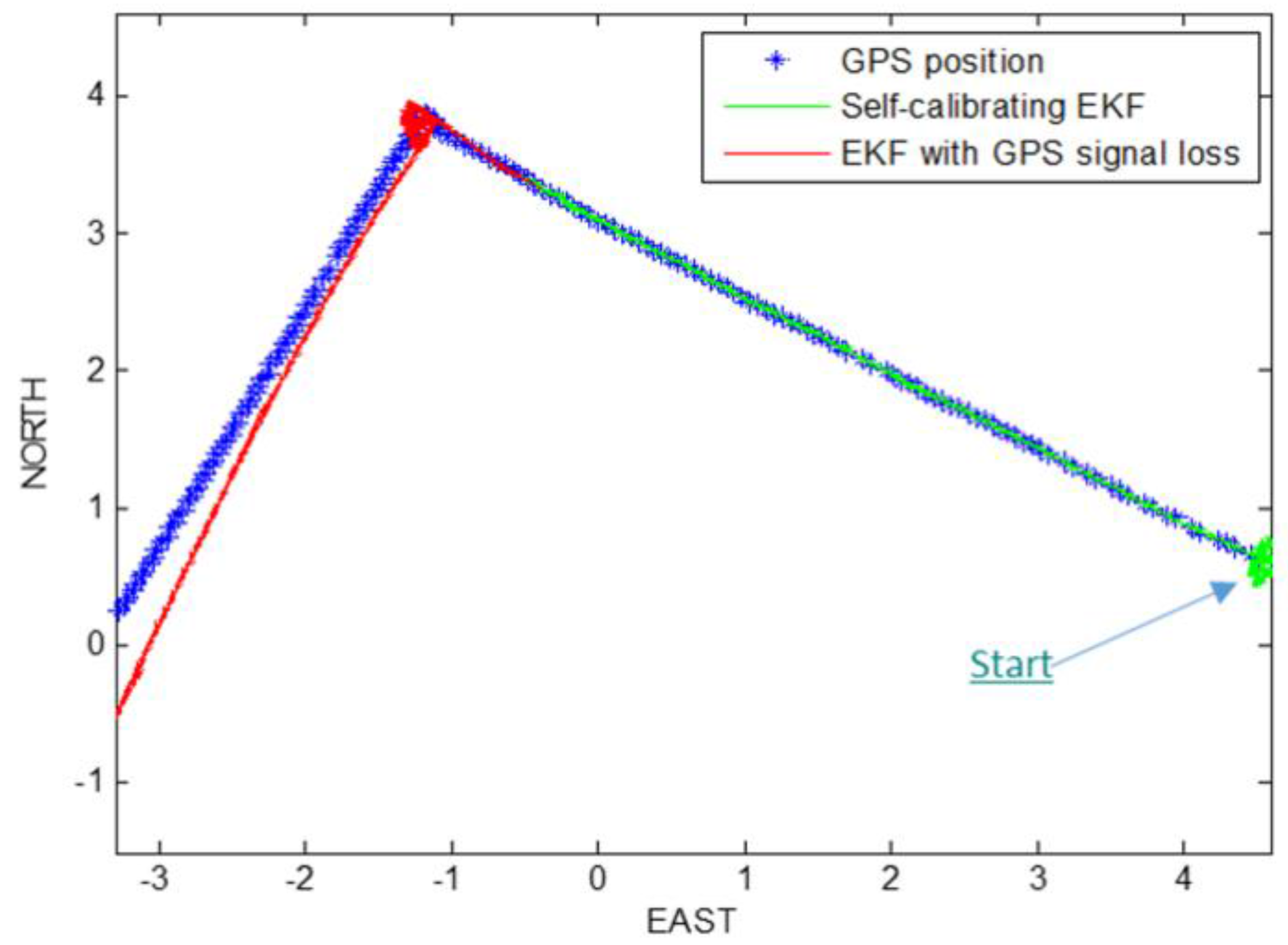
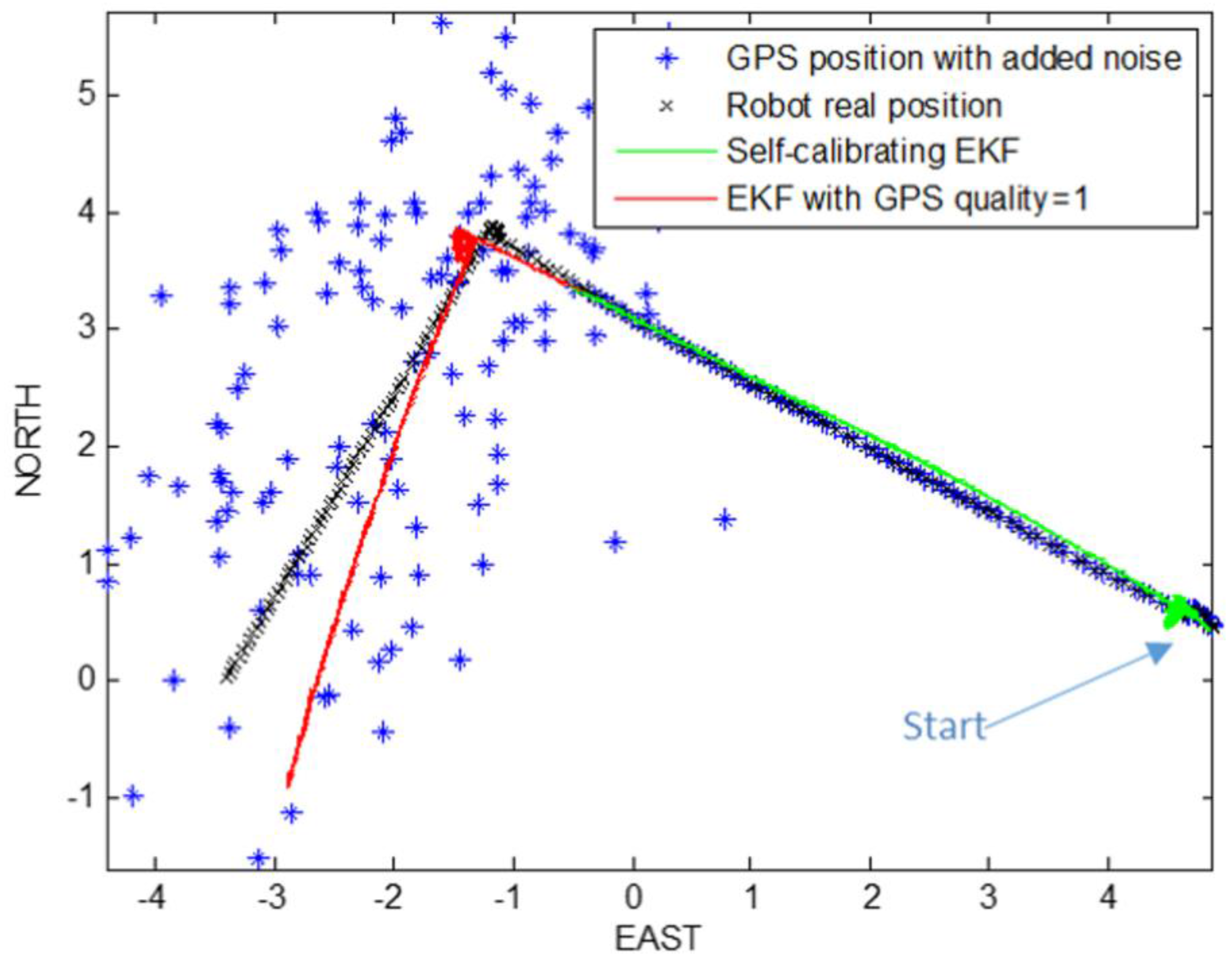
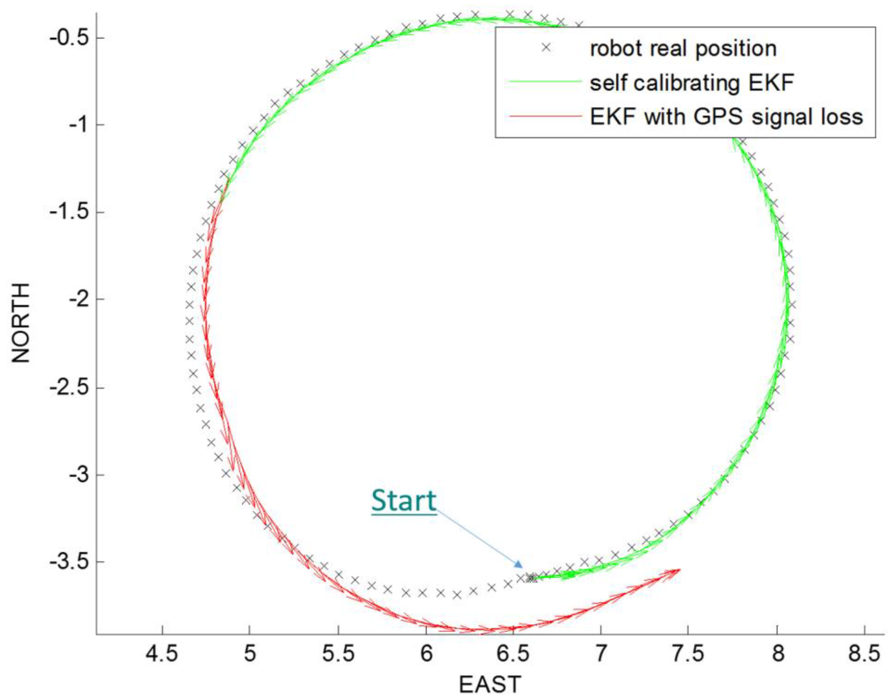
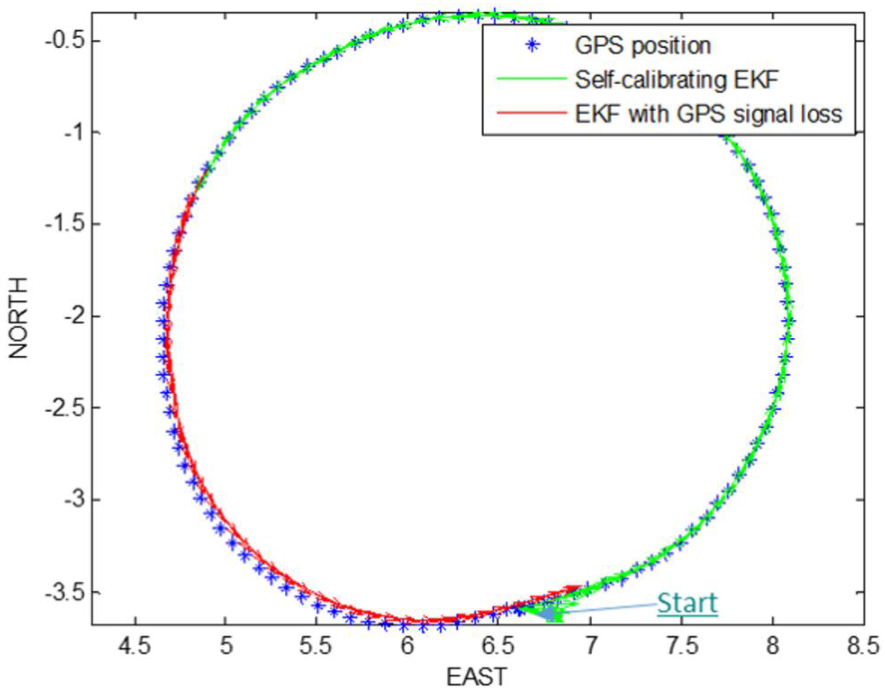
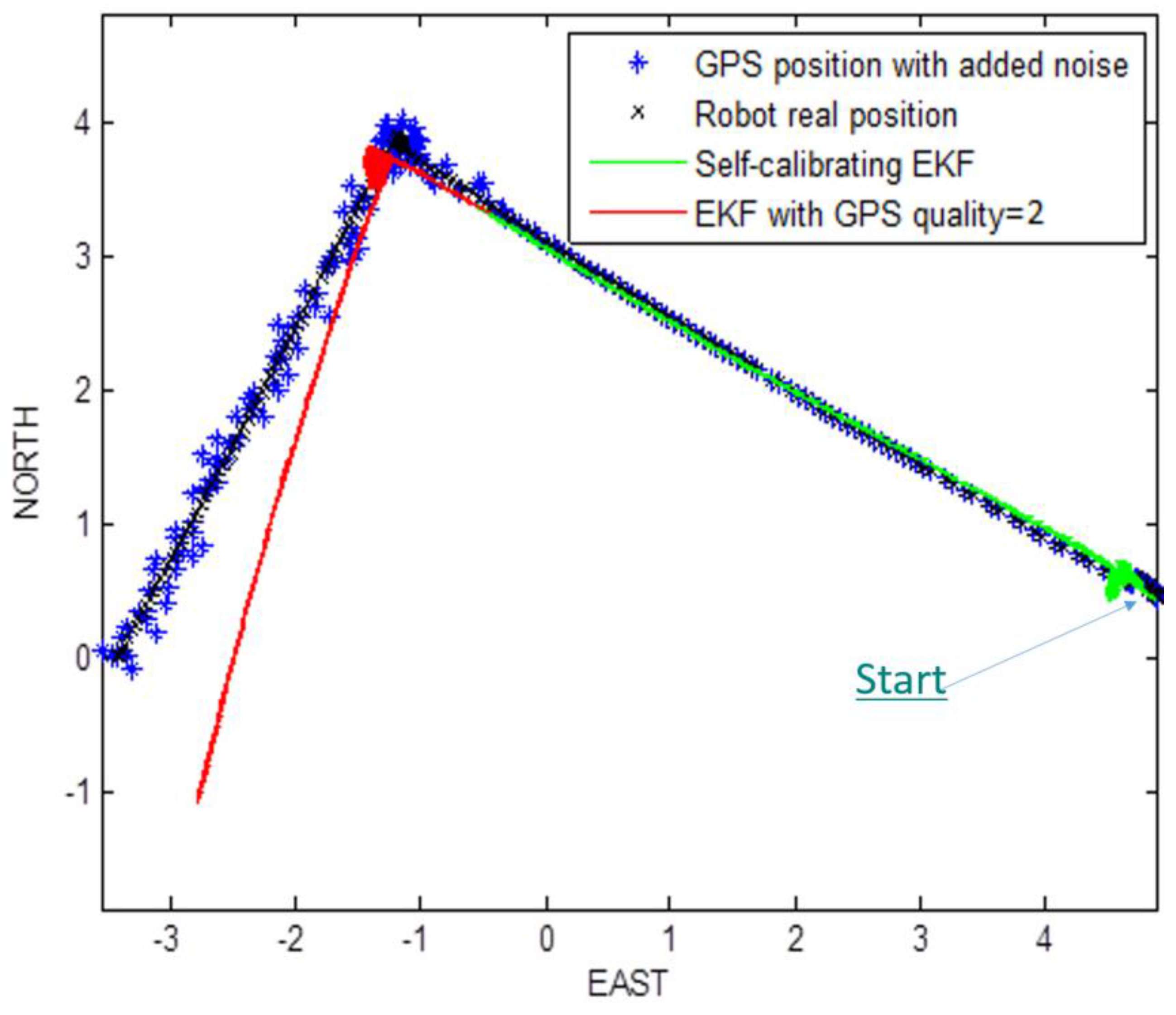
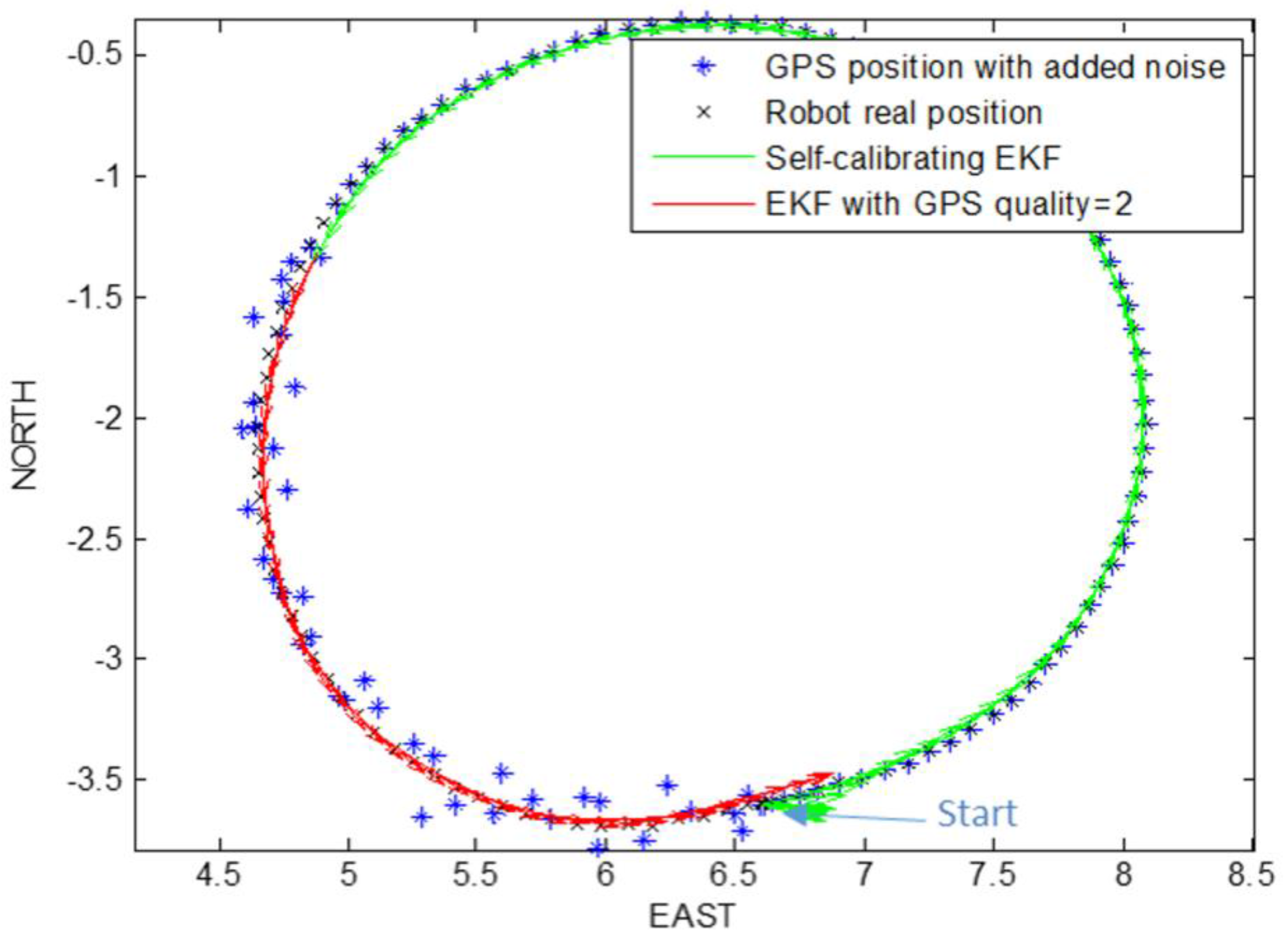
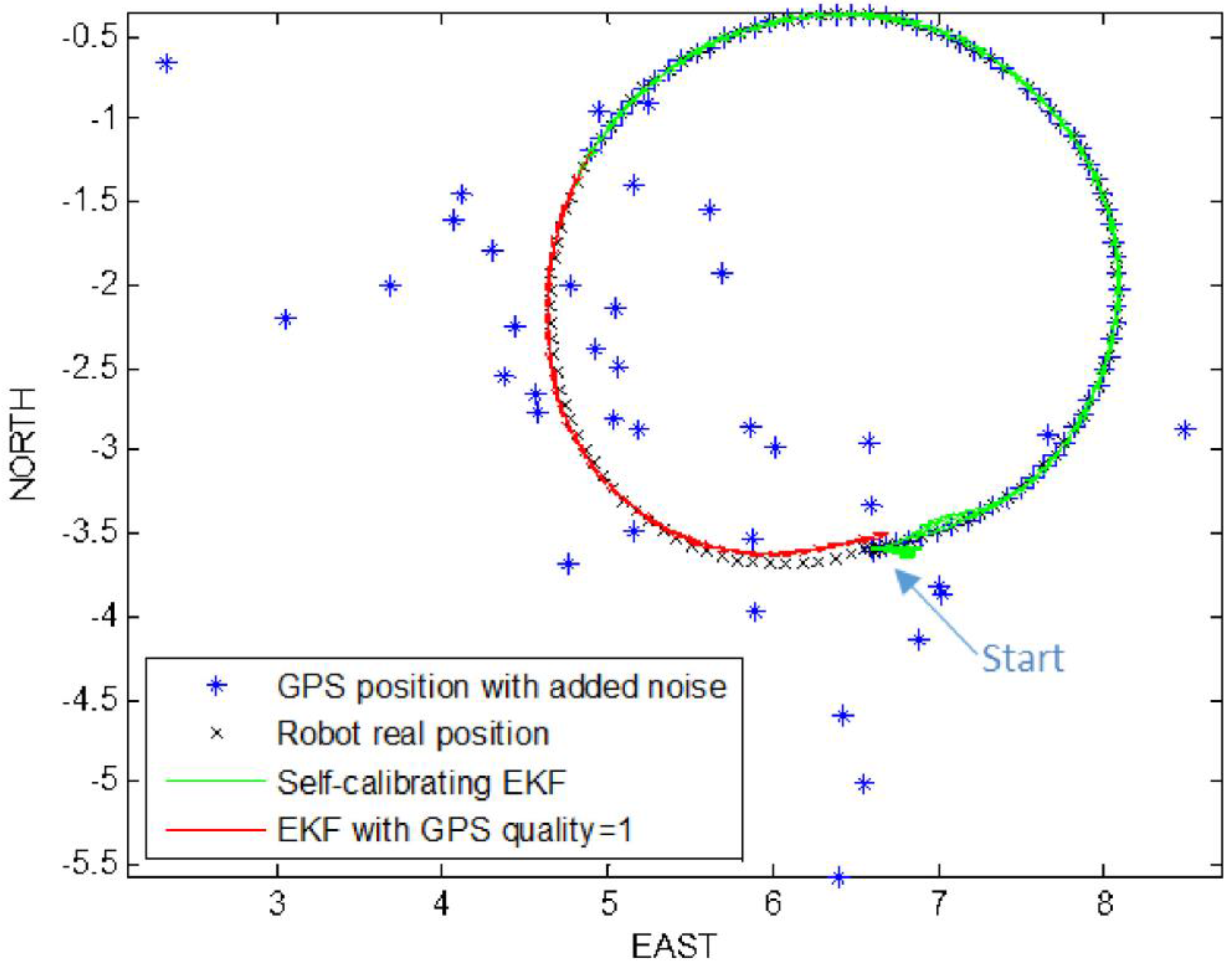
4.1. Experiment 1: Self-Calibrating EKF with GPS Signal Loss
Taking into account the real position and yaw angle of the mobile robot, at the beginning we started the path prediction and correction with the self-calibrating EKF. At a certain time, we simulated a loss of the GPS signal by interrupting the GPS updating phase of the filter, in order to reconstruct robot path only with encoders and AHRS platform data, taking into account also the estimation of robot parameters, which are also the last three elements of the state vector:
. The
Figure 3,
Figure 4,
Figure 5 and
Figure 6 show the path reconstruction without GPS updating phase of EKF (red path), highlighting the advantages of the offset estimation. All the measurements are reported in meters.
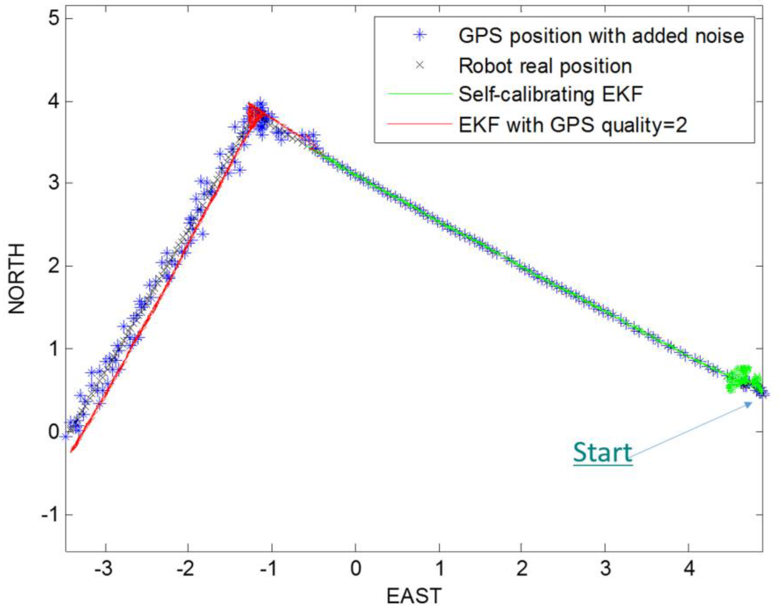
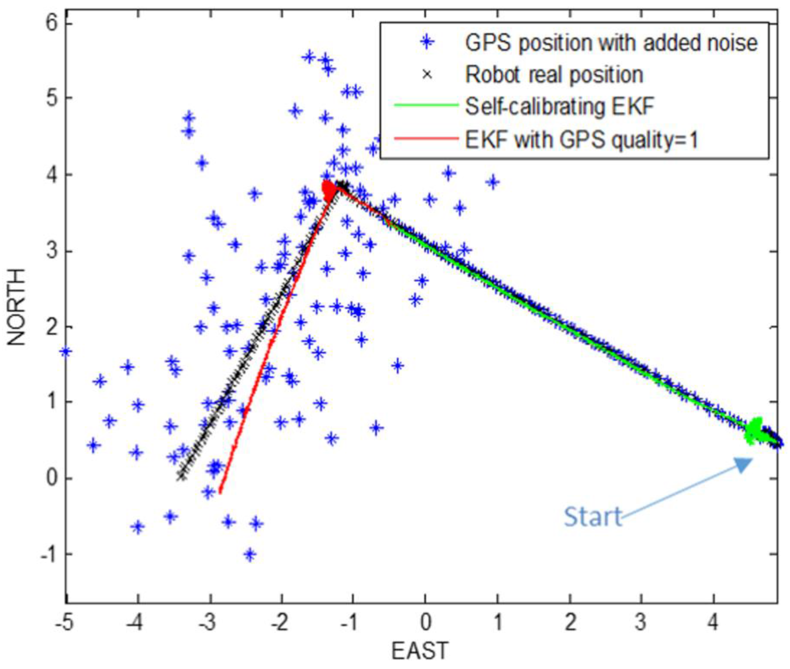
4.2. Experiment 2: Decrease of GPS Signal Quality Simulations ()
Taking into account the real position and yaw angle of the mobile robot, at beginning we start the path prediction and correction with both the self-calibrating EKFs. At a certain time, we add a white Gaussian noise, with
(GPS fix quality = 2), and so affect the GPS position coordinates, in order to simulate a decrease in the GPS signal quality. In this way, EKF has to reconstruct robot path and to estimate robot parameters, taking into account the added noise. The
Figure 7,
Figure 8,
Figure 9 and
Figure 10 show the noise addition in the GPS data, and the results of both algorithms.
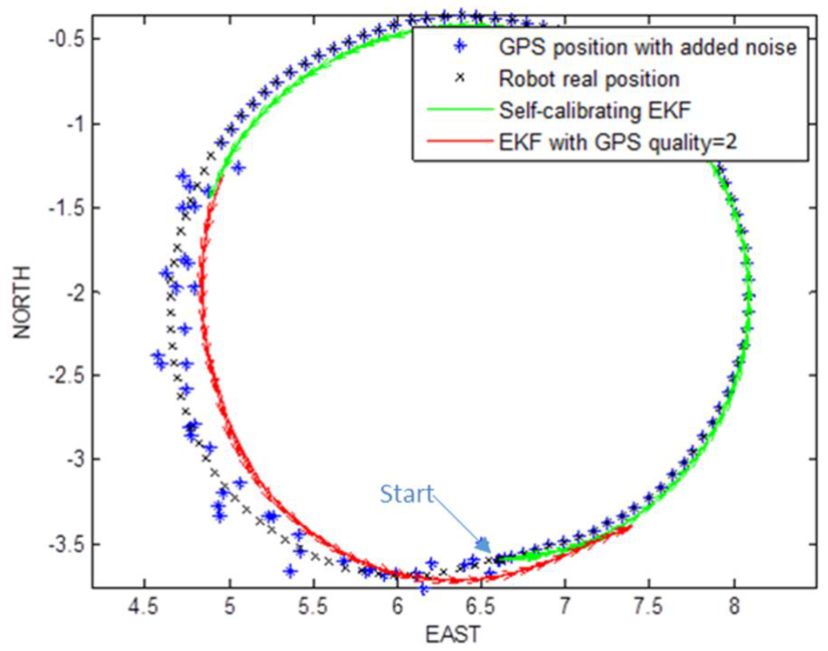
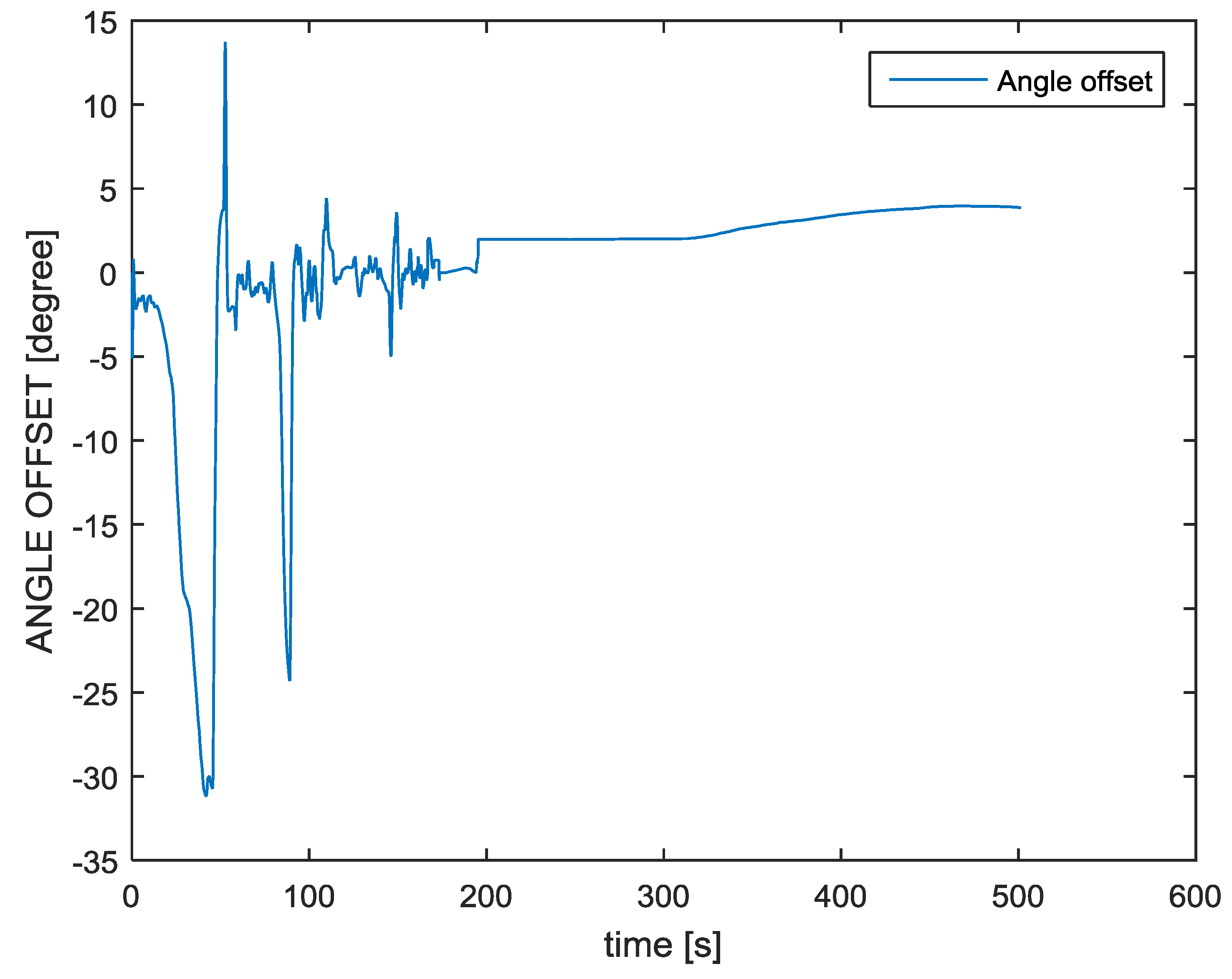
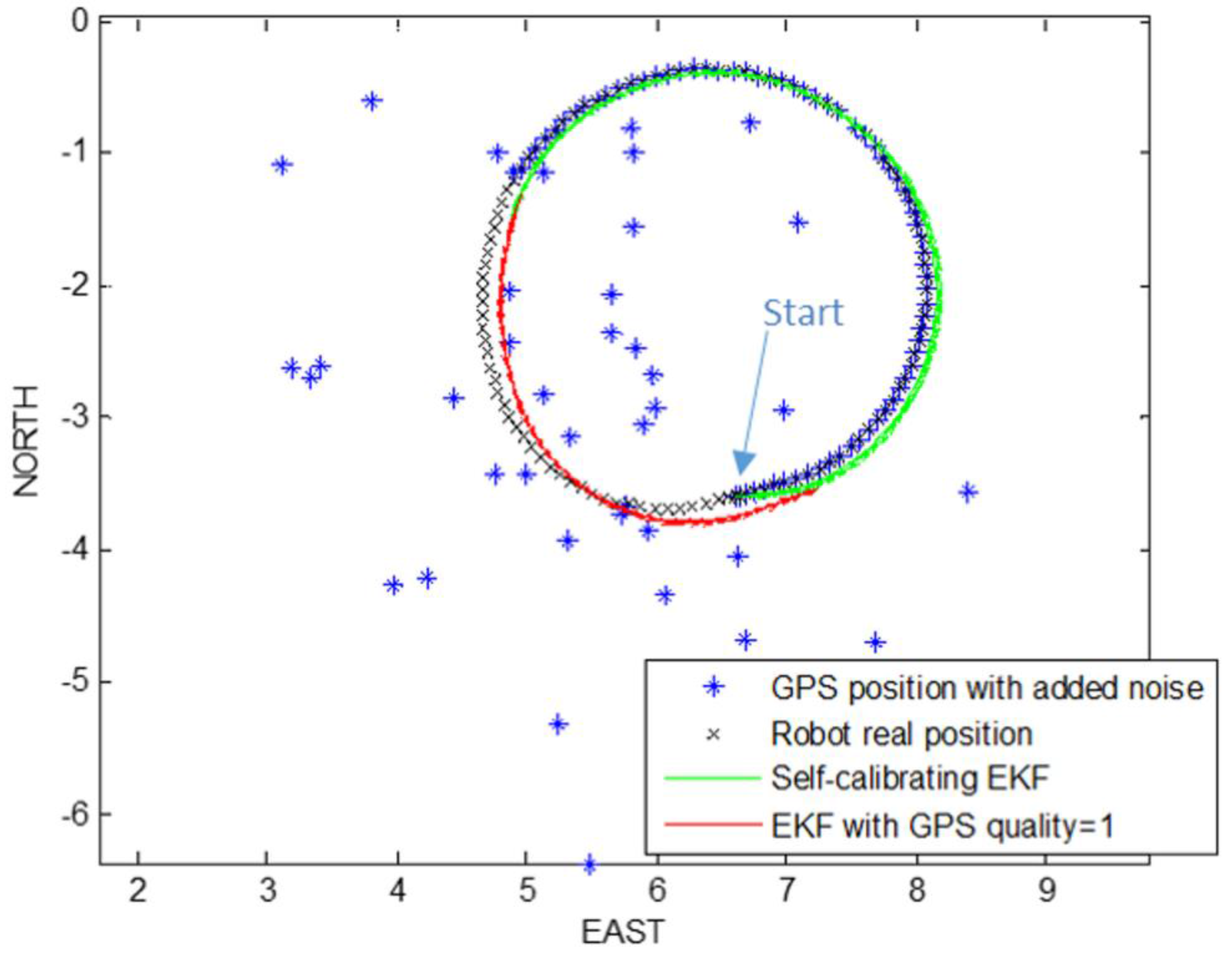
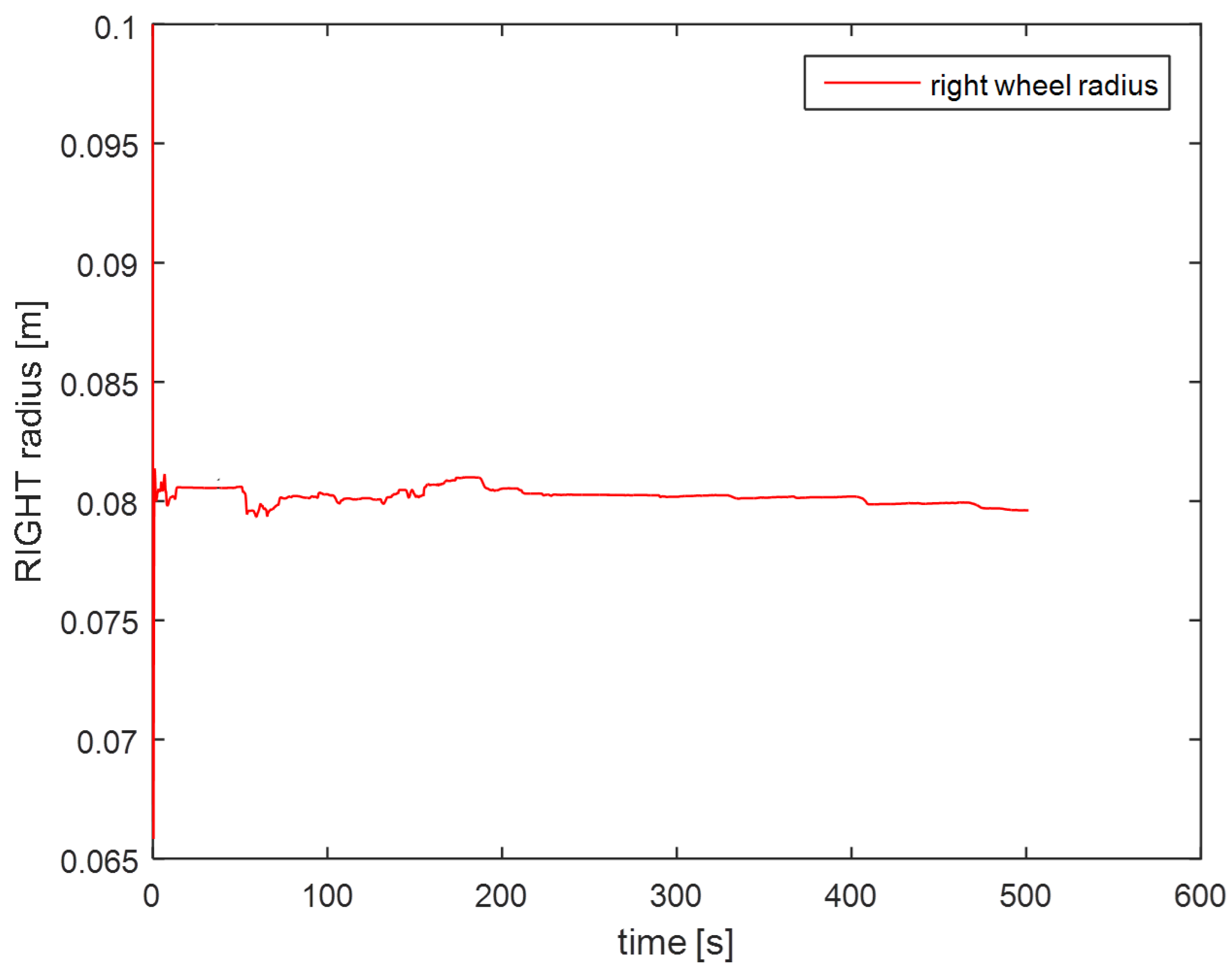
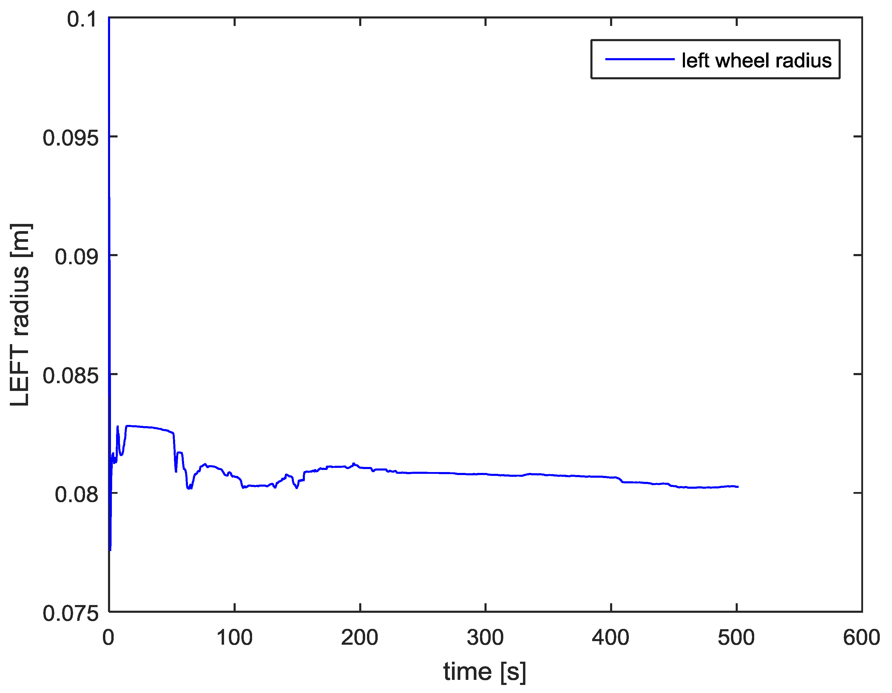
4.3. Experiment 3: Self-Calibrating EKF with Offset Estimation and a Decrease of GPS Signal Quality Simulations (σnoise = 5 m)
In this experiment a large white Gaussian noise, with (), was added to GPS measurements (GPS fix quality = 1).
Also in this case the algorithm does not only estimate only the robot parameters , but also the angle offset, that we want to compensate. In this way, the trajectory reconstruction is made by considering this term for each step, with an improvement of the performance.
The
Figure 11,
Figure 12,
Figure 13 and
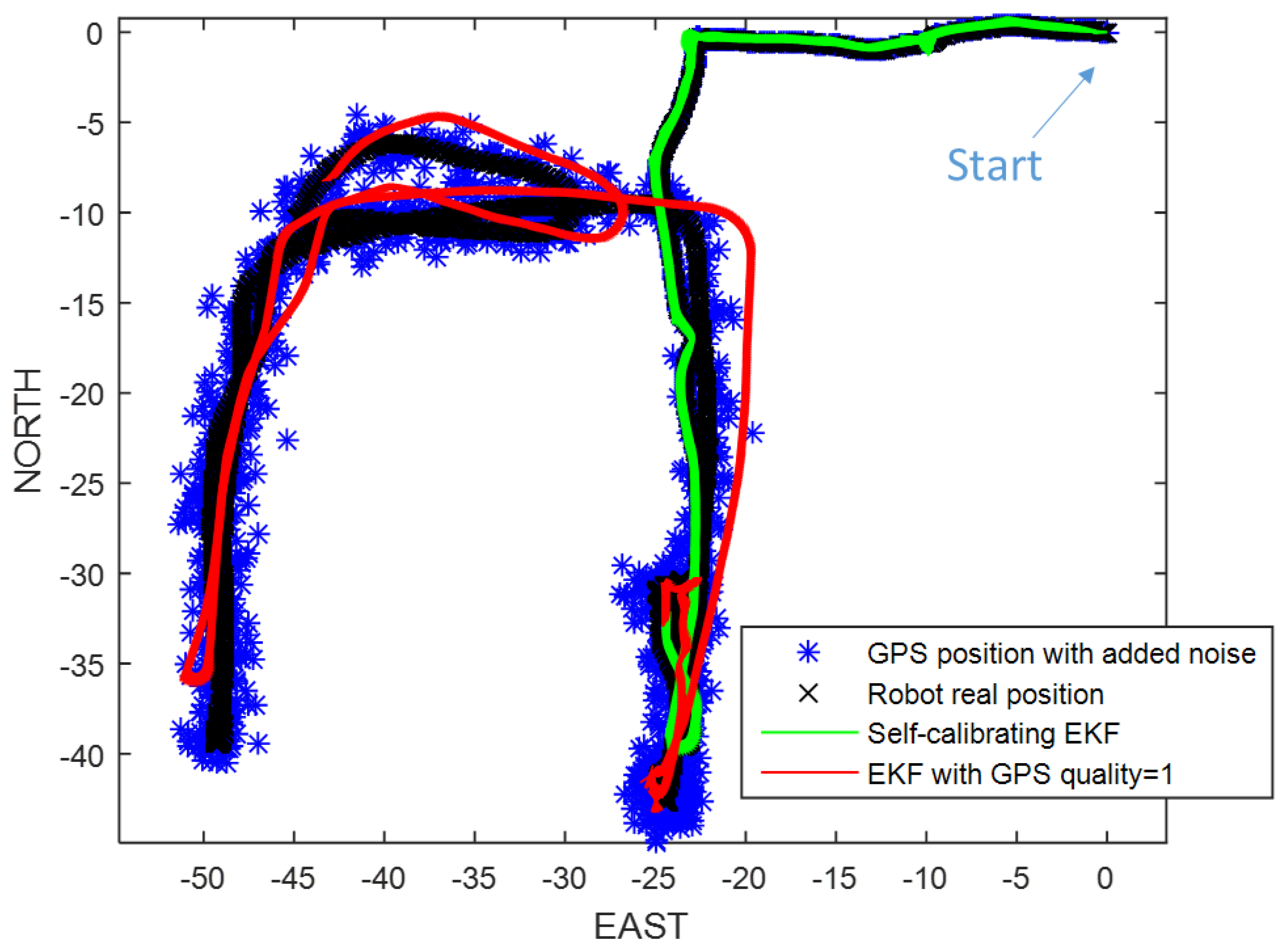
Figure 14 show the estimated trajectories for rectangular and circular path. Finally the methods have been tested in a general-shape path where there are several changes of direction (see the
Figure 15). The
Figure 16 and
Figure 17 show the performance of the methods, without and with offset estimation respectively, while
Figure 18,
Figure 19,
Figure 20 and
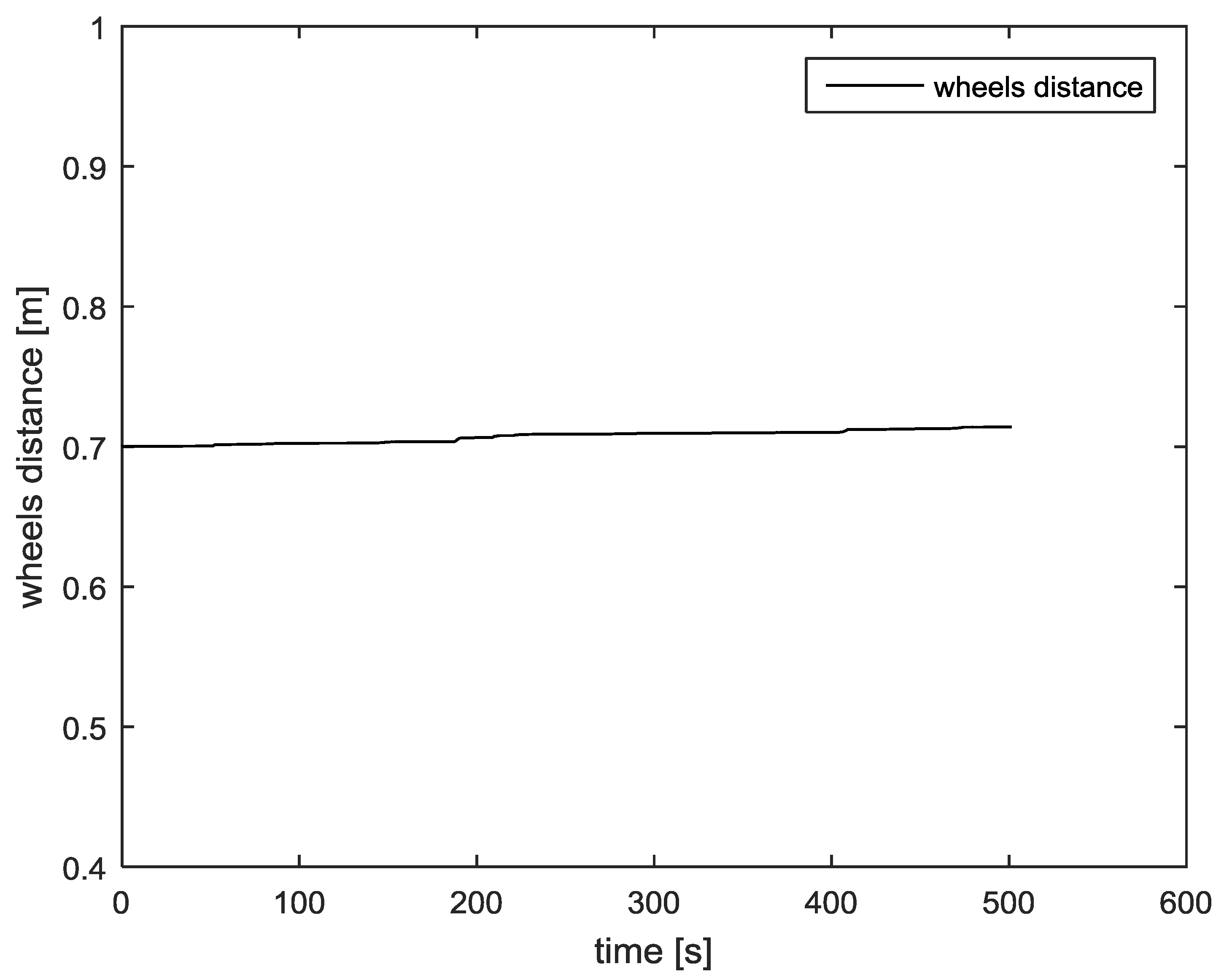
Figure 21 show the estimated parameters in the last case. Observe how, after a short transient, the parameters rapidly converge.
5. Conclusions
From a careful analysis of the results, it is possible to observe, the great improvement of the self-calibrating EKF algorithm, in terms of path reconstruction, by adding the estimation and compensation of the robot orientation angle offset. It is possible to observe, also, the good estimation ability of robot parameters, which values are, at the end, very close to their measured dimensions:
Taking into account the influence of the magnetic structures near or inside the robot to the magnetometer, the basic self-calibrating EKF showed several drawbacks. Indeed, looking at the kinematic model of the robot (used in the EKF algorithm), it is possible to see that the angle term—the orientation of the robot—is present in X and Y position equations. This means that if we have errors about yaw information, its position will also have a wrong result, because simulating a GPS signal loss, or a GPS signal quality decrease, the algorithm should reconstruct robot trajectory only taking into account encoders data. However, the odometry is not sufficient, because it is low precise, considering errors depending by sliding behavior of tracks, digital sampling, and so on. In addition, the uncertainty of odometric measurements grows with the distance. Therefore, taking into account a failure or low-quality of the GPS signal in the algorithm, it is necessary to estimate, step by step, this disturbance value, in order to compensate it and to obtain robot position reconstruction with more precision.
The proposed algorithm allows reducing such errors and the experimental results presented confirm the suitability of the proposed approach. The presented results, by introducing the compensation of the magnetometer offset extend and improve the method of [
5,
9].


