Visual Tracking of Deformation and Classification of Non-Rigid Objects with Robot Hand Probing

Abstract

Performing tasks with a robot hand often requires a complete knowledge of the manipulated object, including its properties (shape, rigidity, surface texture) and its location in the environment, in order to ensure safe and efficient manipulation. While well-established procedures exist for the manipulation of rigid objects, as well as several approaches for the manipulation of linear or planar deformable objects such as ropes or fabric, research addressing the characterization of deformable objects occupying a volume remains relatively limited. The paper proposes an approach for tracking the deformation of non-rigid objects under robot hand manipulation using RGB-D data. The purpose is to automatically classify deformable objects as rigid, elastic, plastic, or elasto-plastic, based on the material they are made of, and to support recognition of the category of such objects through a robotic probing process in order to enhance manipulation capabilities. The proposed approach combines advantageously classical color and depth image processing techniques and proposes a novel combination of the fast level set method with a log-polar mapping of the visual data to robustly detect and track the contour of a deformable object in a RGB-D data stream. Dynamic time warping is employed to characterize the object properties independently from the varying length of the tracked contour as the object deforms. The proposed solution achieves a classification rate over all categories of material of up to 98.3%. When integrated in the control loop of a robot hand, it can contribute to ensure stable grasp, and safe manipulation capability that will preserve the physical integrity of the object.

1. Introduction

Object manipulation is one of the fundamental capabilities of autonomous robot systems, yet the design and development of autonomous robotic systems able to manipulate objects, in particular deformable objects, without human intervention is still a challenging area of research. In order to achieve efficient and safe manipulation, a complete knowledge of the manipulated object is often required. In contrast to the manipulation of rigid objects which is extensively studied in the literature, and for which well-established procedures exist, the investigation of the manipulation of deformable objects represents a more recent undertaking. Several 1D and 2D solutions have been proposed to tackle the issue of grasping and manipulation of soft objects [1,2,3] such as pieces of fabric or ropes. On the other hand, researchers have only recently addressed the manipulation and grasping of fully shaped 3D objects [4,5,6,7,8,9,10] and mostly focused on modeling the behavior of the deformation, or detecting and ensuring stable grasp. Limited solutions yet exist for the automated classification of deformable objects in accordance with different materials they can be made of, forming classes of elastic, plastic, elasto-plastic, or rigid objects, each category calling for different handling strategies. The characterization generally involves the approximate identification of elastic parameters of a formal model, often a mass-spring model [6,11], a finite-element (FEM) representation [6,12,13], or an elaborate surface mesh model [14,15]. Parameters are typically estimated by comparing the real and simulated object subject to interaction and aiming to minimize the differences between the two. However, these approaches require that assumptions are made on the object material, such as linearity, homogeneity or isotropy, which are inadequate for several real-world materials (e.g., foam, rubber) for which the elastic parameters are difficult to define properly. This motivates the development of methods that do not attempt to formally model the material of the object, but rather employ a data-driven approach to make decisions based on the observed properties of the object, capture implicitly its deformation behavior, and support adaptive control of a robotic hand.

In this context, the main goal of this paper is to present the development and implementation of a framework that enables the characterization of generic deformable objects by visually observing their interaction with a robotic hand. Generic objects considered here are objects that physically occupy a 3D volume, rather than planar fabric or one-dimensional ropes. This work represents a first step toward a model-free characterization of the deformation behavior of objects under robot manipulation. As such, assumptions are for now made on the availability of a 2D contour surrounding the object as perceived from the camera point of view, in order to develop the technology and prove its feasibility. The expected use of the solution is for a robot hand to probe an unknown and unmodeled deformable object and then automatically adapt the hand behavior, such as the grasping strategy and the magnitude of applied forces, according to the object’s characteristics. When integrated in the control scheme for a robotic hand, the solution contributes to ensure stable grasp and precise manipulation capability without a priori knowledge of the shape and material of the object. This technology can contribute to enable autonomous robots to handle and interact efficiently with unknown objects. This paper does not investigate the problem of object manipulation in a comprehensive manner, but rather focuses on the experimental determination of deformation characteristics for objects made of different materials, without making use of formal modeling. Questions related to object’s pose determination, contact points distribution [16], and manipulator path planning are not addressed here, as numerous solutions already exist in the literature about these issues.

The proposed procedure makes use of the depth and color image data returned by a Kinect sensor properly positioned to observe the robotic hand that performs the deformable object probing. Segmentation and background removal are conducted with the well-known random sample consensus (RANSAC) [17] and k-d tree search [18] algorithms applied over the depth point cloud. The corresponding points from the color image are encoded in the YUV color space and mapped in the log-polar domain [19]. The fast level set method [20] for contour detection and tracking is then applied on the log-polar map. The original combination of level sets with log-polar domain representation of visual data enables a robust contour identification and subsequently the tracking of the deformations in the data stream. Capitalizing on the behavior of the contour during the probing phase, the object gets classified as belonging to the rigid, elastic, plastic or elasto-plastic class of deformable objects, using a solution based on dynamic time warping [21]. The purpose of this characterization is to enable better manipulation capabilities for a robot hand by dealing efficiently with deformable objects composed of different materials that impact their physical behavior.

The contributions of the paper provide an original framework for characterizing deformation properties (and stages of deformation) of an object under interaction with a robot hand using RGB-D data. The original application of the fast level set method in the log-polar representation of the color map to capture and track the object contour during deformation proves robust and efficient. Also, a decision system based on dynamic time warping to characterize the object’s deformation properties independently from the length of the contour, and possible movement of the object under manipulation, provides a complete solution for the characterization of a variety of deformation behaviors.

2. Literature Review

This section summarizes the most relevant related work on object material characterization and on robotic manipulation of deformable objects. The work of Petit et al. [5] considers RGB-D sensor data for tracking of 3D elastic objects. The approach assumes that a prior visual extraction of the object of interest is available, and the ICP algorithm is applied on the resulting point cloud to estimate a rigid transformation from the point cloud to a linear tetrahedral FEM model representing the object. Linear elastic forces exerted on vertices are computed from the point cloud to the mesh based on closest point correspondence and the mechanical equations are solved numerically to simulate the deformed mesh. This work is restricted to elastic objects. Zaidi et al. [6], without capturing visual data, model a linear isotropic 3D deformable object in interaction with a three-fingered robot hand as a mass-spring system based on a tetrahedral mesh. The estimation of contact points and object deformations is based on tracking the node positions and solving the dynamic equations of Newton’s second law. In [10], the stiffness of a 3D planar elastic object is measured by the curvature of surface points from the object geometry. The local deformation is described in terms of a level curves set. The work is further expanded in [22] to supervise the grasping of a non-rigid object and provide the robot controller with signals when deformation is detected. The process is interesting in that it does not require a formal model of the object deformation or of its material. However, it is not meant to provide differentiation between various categories of deformable objects. Elbrechter et al. [11] model a piece of paper in interaction with a robot hand as a 2D grid of nodes connected by links that specify the bending constraints, namely a resting distance between two nodes, and use a stiffness coefficient. The parameters are tuned manually. Markers are inscribed on the surface of the paper to track its folding in the visual input. Choi et al. [23] track the global position of moving deformable balls, painted in red against a blue background, in a video stream and adjust the elasticity parameters of a mass-spring model of the ball by optimizing the differences with the real object. In Kraft et al. [24], sparse sets of oriented 3D points along contours of objects manipulated by a robotic manipulator are monitored using a stereo camera and then predicted based on the motion induced by the robot. Schulman et al. [13] track deformable objects from a sequence of point clouds by identifying the correspondence between the point cloud and a model of the object composed of a collection of linked rigid particles, governed by dynamical equations. An expectation-minimization algorithm aims at finding the most probable node positions for the model given the measurements. Tests are performed in a controlled environment, against a green background that limits its applicability to normal conditions. In [25], a solution is proposed for the robot manipulation of elastic objects that allows controlling simultaneously the object’s final position (i.e., interest points over the object and its centroid) and its deformations. The latter are represented as the compression distance between points of interest, the folding angle and the normalized curvature of the object, as estimated by the curve passing through three interest points. The solution is however limited to elastic deformations only. An approach that does not assume a prior model or template for the object is proposed by Hur et al. [26]. They introduce a 3D deformable spatial pyramid model to find the dense 3D motion flow of deformable objects in RGB-D data. The point cloud is corrected with a depth hole-filling algorithm and treated with a Gaussian filtering prior to the computation of a series of perspectively normalized descriptors. The 3D deformable spatial pyramid finds dense correspondences between instances of a deformed object by optimizing an objective function, in form of an energy corresponding to a Markov random field, taking into consideration factors such as translation, rotation, warping costs and descriptors matching costs.

3. Proposed Approach for Deformation Tracking and Material Classification from RGB-D Data

The proposed system for object deformation monitoring and classification from RGB-D data is illustrated in Figure 1. It takes as inputs the RGB image and the corresponding depth point cloud collected by a Kinect sensor, and a user selected 2D fixation point in the RGB image that guides the system towards the location of the object of interest. Based on the provided inputs, in the initial step only, a 3D fixation point is calculated from the 2D fixation point provided by the user, using 2D-3D mapping in the RGB-D data. The depth point cloud recuperated from the Kinect is subject to a background removal operation using the RANSAC algorithm [17]. The main purpose of this operation is to remove from the scene any undesirable elements (e.g., measurement table or robot hand mounting plate, and other measuring equipment visible in the RGB-D data stream) in order to better identify the object shape and thus reduce the processing time. Then, a cluster representing the object is extracted based on the computed 3D fixation point from the remaining part of the point cloud after background removal. The identified 3D object cluster is projected back to 2D and the resulting projection is used to compute a bounding window in the color image around the identified object. The region within the bounding window is encoded in the YUV color space before being further processed. This YUV coded area of interest is projected in the log-polar domain to create a cortical image before a fast level set method is applied on it to extract or track the contour of the object. The cluster from the color map resulting from the 3D-2D projection serves for the first initialization of the level set contour tracking method. The resulting object contour is then converted back to the RGB image Cartesian coordinates for visualization. After the initial frame is processed, the region extracted from the last processed image replaces the initial cluster in the color map and provides the level set re-initialization data for the following frame in the sequence to be processed with the level set method. The process then repeats over the entire sequence, within the YUV encoded window that is captured from the current image, with the same size as the first bounding window, and which gets mapped in the log-polar domain. The initial fixation point selection, background removal, and clustering operations are not performed on successive images.

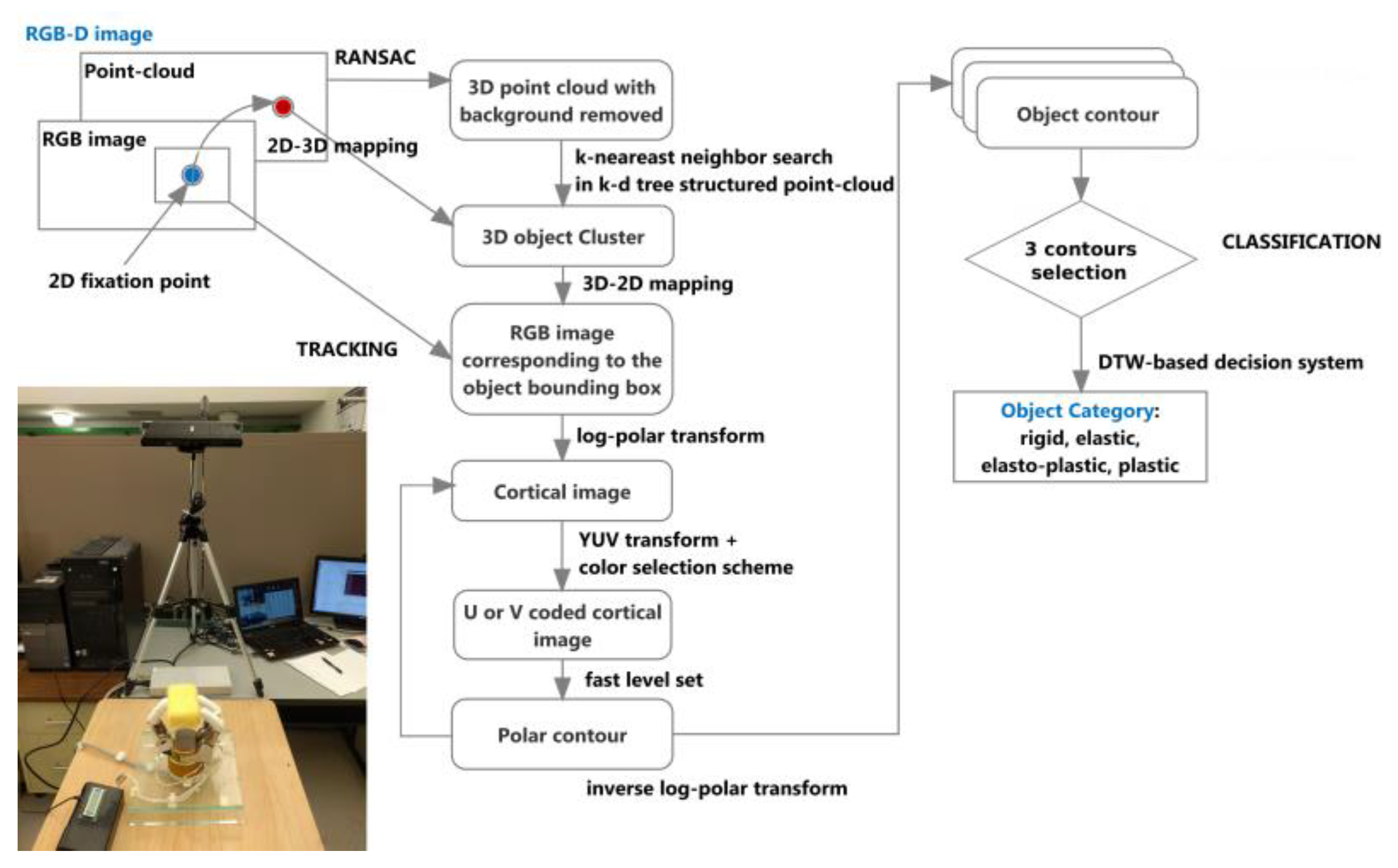
In a separate step, after all frames have been processed, three representative frames and their corresponding contour maps are extracted from the sequence and the object material is classified based on the behavior of the contour during the manipulation with the robot hand. Four categories can be identified: rigid, elastic, plastic, or elasto-plastic objects. A dynamic time warping (DTW) approach is applied to perform this classification task.

3.1. Initialization Stage

Upon analyzing a sequence of RGB-D data, a user-selected point is fed in the system to initially guide the algorithm towards the location of the object of interest. This selection is only required in the first frame of the data stream and allows the system to rapidly locate the deformable object independently from its color, shape, location or orientation in the workspace, and also independently from the complexity of the background or from the relative configuration of the robot hand and Kinect sensor. Such user guidance is common in the current feature tracking literature, but in many cases is more extreme than what is required in the proposed solution. For example, a prior selection of the object of interest is assumed to be available in [5], or the user is asked to crop the object in the initial frame in [23]. In our case, a single fixation point is needed and it can be selected randomly over the object of interest. Its coordinates are used by the system to indicate the general location of the object. Experiments demonstrated that while the algorithm works regardless of the position of this point over the surface of the object of interest, a 2D fixation point, ${\mathit{p}}_{2D}$, chosen roughly at the centre of the object leads in general to more accurate contour estimation. 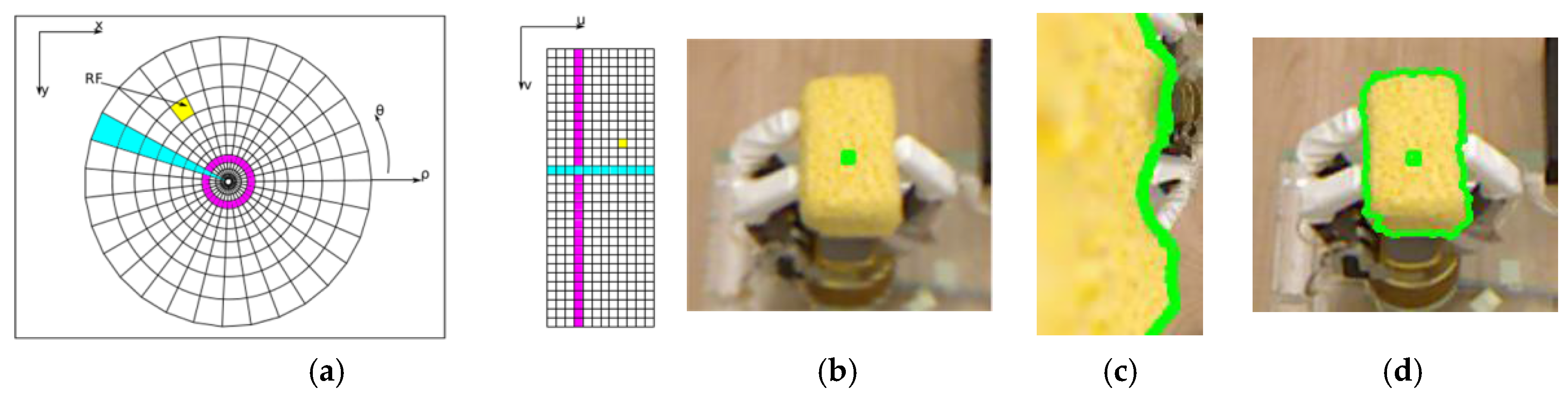The idea of using a central fixation point is inspired by the work of Mishra and Aloimonos [27]. The authors suggest that human retina fixates an interesting object with a high resolution captured by the fovea and the rest of the visual information at lower resolution. In the current work, this process is replicated by the use of a log-polar mapping to perform contour detection and tracking. In the log-polar map, the 2D fixation point represents the centre of the transformation, where the precision of the log-polar image is maximal.

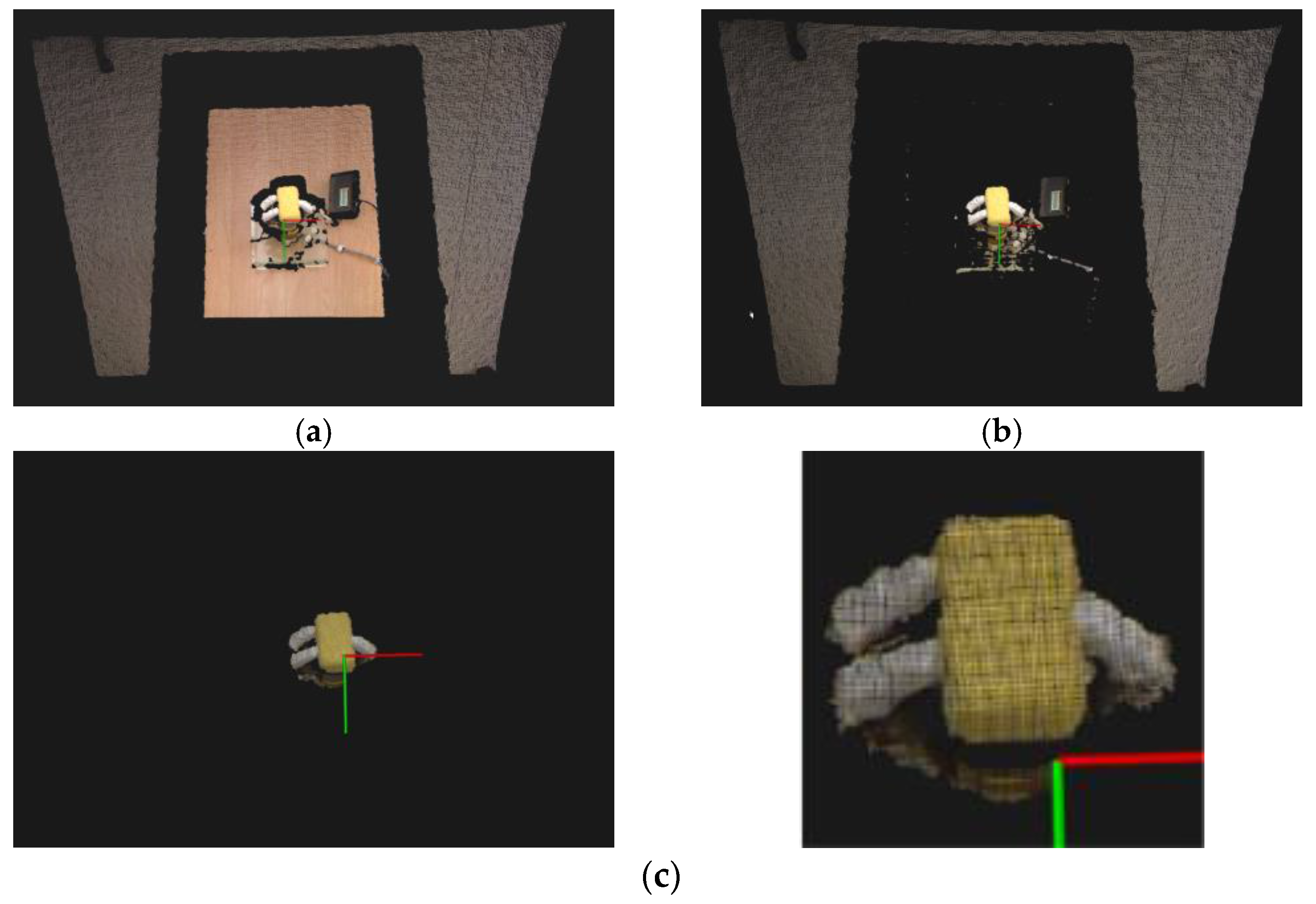
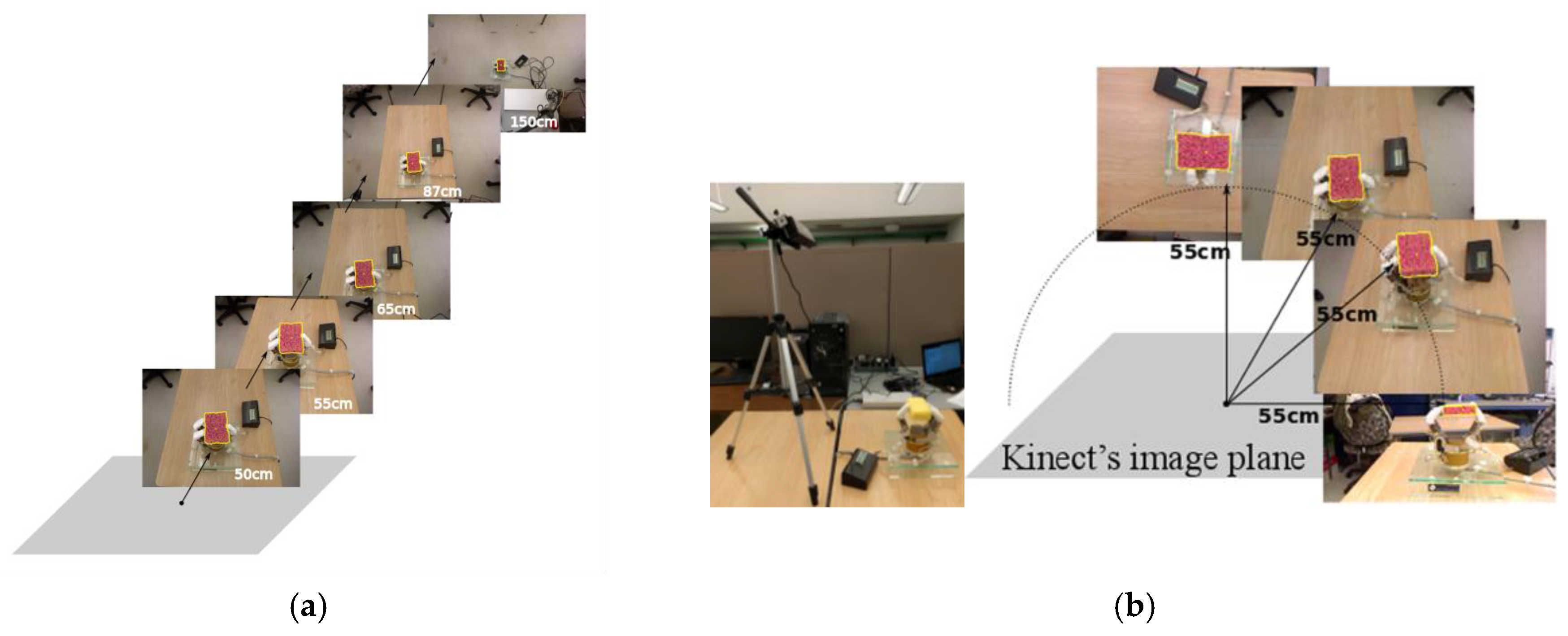
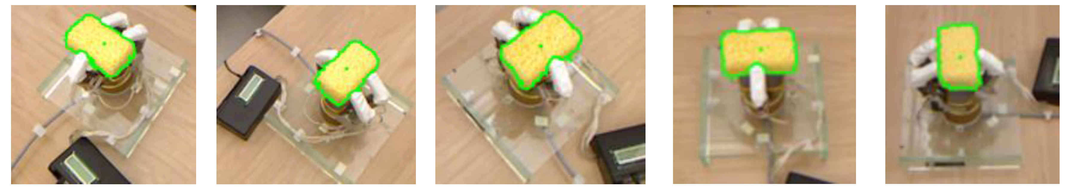
A 2D-3D mapping that takes into consideration the intrinsic calibration parameters of the Kinect sensor [28] is applied to estimate the 3D fixation point, ${\mathit{p}}_{3D}$, in the point cloud corresponding to the 2D fixation point, ${\mathit{p}}_{2D}$, in the color image. The initial goal is to separate the points representing the object of interest from the background in the RGB-D data stream. During experimentation the object is placed in a robot hand situated over a table (Figure 1) and pointing upward while manipulating the deformable object, and a Kinect sensor is positioned above the scene. Under the current assumptions, an efficient way to remove most of the background is to locate the planar surface representing the table and to extract that surface from the RGB-D data. This surface is the one closest to the object and its identification improves the definition of the area in which the object lies. In a more general context where the robot hand would reach to manipulate an object in any location in space, an equivalent background removal procedure could consist of applying a threshold on the distance map to remove all surfaces located behind the object of interest. However, this would also impose strategically positioning the RGB-D sensor according to the object location, which remains beyond the scope of the current research.

Under the consideration of a planar surface behind the manipulated object, the planar surface identification is viewed as a plane-fitting problem which can be resolved with the RANSAC algorithm [17]. The approach, implemented as per the “plane model segmentation” and “extracting indices from a point cloud” algorithms of the Point Cloud Library (PCL) [29,30], is applied over the 3D point cloud in the RGB-D data stream. Given that at least three non-collinear points are required to estimate the plane model, the minimum size of the sample set, s, is set to 3. The distance threshold is chosen empirically and set to t = 1 cm to ensure a good balance between the background table removal and processing time. An example of the reduced point cloud, $C^{*}$, after removal of the table and background visible in Figure 2a, is shown in Figure 2b.

The next step consists of narrowing down the search area to the object of interest in the reduced point cloud, $C^{*}$. The purpose of this step is to extract a single cluster containing the nearest elements to the fixation point identified by the user in a Euclidean sense and that represents the object of interest. The solution capitalizes on a k-d tree structure and the use of the fixed-radius near neighbors search algorithm. Because an estimation is used to approximate the location of the 3D fixation point from the 2D-3D mapping described previously, and also due to the errors on depth that characterize the Kinect sensor, the estimated 3D coordinates, ${\mathit{p}}_{3D}$, may not exactly correspond to an existing point in the point cloud. Moreover, because the point cloud recuperated is unstructured, in order to find the neighbor of each point, the k-d tree data structure supports a faster nearest neighbor search. Therefore, a k-nearest neighbors search [18] is applied to identify the k-nearest points, $inX$, in the reduced point cloud, $C^{*}$, to the estimated 3D fixation point, ${\mathit{p}}_{3D}$. An empirically chosen value of k = 100 is used to accelerate the computation of the clustering approach while also guaranteeing that the cluster of the object of interest contains at least 100 points. Beginning with these 100 points, the neighborhood of each is further researched for extra points located within a maximum distance, $d_{th}$, which can be integrated in the object cluster. A value of $d_{th}$ = 5 mm was empirically determined. The resulting object cluster is therefore composed of the initial 100 points augmented by any other points discovered within the distance threshold, $d_{th}$. The merging condition for the clustering is the Euclidean radius. The algorithm used slightly differs from that available in the PCL library [30] in that it concentrates on a single cluster located around the user-determined fixation point. Algorithm 1 summarizes the process.

Algorithm 1. 3D cluster extraction algorithm.

Input:

Point cloud $C^{*}, C^{*}=\left\{{\mathbf{p}}_i\right\}$ representing the point cloud after table removal

$inX$ = set of k-nearest-neighbors to the estimated 3D fixation point, ${\mathbf{p}}_{3D}$ (with k = 100)

$d_{th}$ = spatial distance threshold for a point to be considered as a neighbor (set to 5 mm)

Output:

The object cluster, $cluster$

function ClusterExtraction ($C^{*}$)

if $C^{*}.empty()$ then

return $\varnothing$

else

Build k-d tree representation of $C^{*}$

Set up priority queue $Q$ of the points that need to be checked, $Q\leftarrow inX$

for every ${\mathbf{p}}_i\subset Q$ do

if all the points in $Q$ have been processed then

$cluster\leftarrow Q$

else

search the neighbors set $P_i^k$ of ${\mathbf{p}}_i$ in a sphere with radius $r<d_{th}$

for every ${\mathbf{p}}_i^k$ ⊂ $P_i^k$ do

if ${\mathbf{p}}_i^k$ has not been processed then

$Q\leftarrow {\mathbf{p}}_i^k$

end if

end for

end if

end for

end if

end function

Once the object cluster in 3D is identified, the corresponding 2D object cluster in the color image is identified with the inverse 2D-3D mapping in order to initialize the level set contour tracking method. For the case of the yellow object shown in Figure 2a, the final object cluster is shown in Figure 2c. The bounding window with which the level set is initialized to process the first RGB-D frame and initiate the contour tracking represents the bounding box of the 2D points (the farthest left, right, up and down locations) enlarged by 50 pixels in all directions. This tolerance of 50 pixels introduces robustness to cases where the object slightly shifts or rotates during manipulation. This initialization also contributes to the acceleration of the contour detection since the initialization area is close to the object of interest.

3.2. Fast Level-Set Method in Log-Polar Domain for Object Contour Tracking

3.2.1. Log-Polar Transform

The log-polar transform simulates some aspects of the human visual model, in which a high resolution around the fovea allows the eye to fixate on an object of interest, while the rest of visual information is encoded at a lower resolution [31]. Given the polar coordinates $(\rho , \theta )=(\sqrt{x^2+y^2}, arctan(y/x))$, calculated from the (x, y) Cartesian coordinates of an image of size M × N pixels, the discrete log-polar transformation to a discrete cortical image of R rings and S sectors is given by [19]:

$$\{\begin{array}{c}u=\lfloor lo{g}_a(\frac{\rho }{{\rho }_0})\rfloor \\ v=\lfloor \frac{S\theta }{2\pi }\rfloor \end{array}$$

(1)

where $\lfloor .\rfloor$ denotes the integer part, $a=e^{ln({\rho }_{max}/{\rho }_0)/R}$ is a parameter representing the non-linearity of the mapping, with ${\rho }_{max}=0.5min(M,N),$ and ${\rho }_0$ represents the radius of the central blind spot such that all pixels in the radius of ${\rho }_0$ are ignored. In the equation above, u ∈ [1, R] and v ∈ [1, S] and the most favorable relationship between R and S is to optimize the pixel aspect ratio close to 1. In particular, the optimal S can be obtained as $S=2\pi /(a-1)$ [32] for a given R, and typically R = ${\rho }_{max}$. Figure 3a shows a template for the mapping of an image from the Cartesian domain to the log-polar domain for R = 12 and S = 31. The fuchsia ring, the cyan sector and the yellow receptive field (RF) in the Cartesian domain correspond to the fuchsia column, the cyan row, and the yellow cell, respectively, in the log-polar domain. The center of the round template represents the area of maximum resolution (the fixation point), with the central blind spot marked as a black circle.

Figure 3b shows an example of a Cartesian image, with the user-selected 2D fixation point shown in green, while Figure 3c represents its equivalent discrete log-polar representation. The advantage of using this transformation is that the object of interest gets to fill a relatively large area of the log-polar image compared to the remaining background area, as can be observed in Figure 3c. Provided that the fixation point is selected relatively centered over the object of interest, the percentage of space occupied by the object of interest in the log-polar map is proportionally larger than in the Cartesian image, as the log-polar map is centered on the fixation point, therefore implementing the suitable mapping at a higher resolution over the region of interest. Moreover, the use of the log-polar mapping simplifies the search for contour points along a somewhat vertical direction for objects that are generally symmetrical, as illustrated in Figure 3c. Finally, the log-polar mapping typically reduces the size of the representation with respect to the original image (e.g., from 187 × 200 pixels to 93 × 167 pixels in the case shown in Figure 3), based on the resolution of the log-polar mapping that optimizes the pixel aspect ratio (as defined above). This further contributes to accelerate the contour retrieval procedure.

3.2.2. Color Space Encoding to Support Level Sets

Instead of directly using RGB color values in the log-polar image (as shown Figure 3c), a transformation to the YUV color space is performed, where Y is the luminance of a color, and U and V represent the two chromatic components. The simplified UV plane offers a more compact and therefore faster solution to process color information. In the current work, either the U or the V component is selected as the feature for the contour detection. As highlighted in Figure 3c, in the log-polar image, the leftmost columns are the ones that are close to the 2D fixation point and the object of interest occupies a large part on the left side of the image. The proposed algorithm for the color space selection therefore initially computes the mean value of each column in the U component and the V component, respectively. Then, standard deviation values of all the mean values are calculated in the U and V components, respectively, over the entire log-polar map. The component (U or V) with the largest standard deviation is selected as the color feature for the level set method. This choice is justified by the desire to work with higher contrast to enable more accurate segmentation. The fact that the luminance component, Y, is not considered in the process also reduces the dependence of the solution on the local intensity of colors due to different illumination conditions and shading effects.

3.2.3. Fast Level Set Method in Log-Polar Domain

The primary objective being to track the contour of an object submitted to external forces in order to differentiate in between rigid, elastic, plastic, and elasto-plastic objects, this study considered various contour representations, either parametric or geometric. Parametric contour models (i.e., active contour models, or snakes) represent the contour in a parametric form. This representation allows direct interaction with the model and can lead to a compact representation suitable for fast implementation [33]. However, snakes tend to be attracted by spurious edges; they sometimes degenerate the shape by shrinking and flattening; the convergence and stability of the contour deformation by minimization may be unpredictable, and they may yield intersecting boundaries in some situations [34]. Finally, they have difficulty in dealing with splitting or merging model parts, a useful property for extracting objects with unknown topology [35], as those aimed for in this work. This difficulty is caused by the fact that a new parameterization must be constructed whenever topology changes occur. Level set (geometric) contour representation partially overcomes the problems associated with parametric models by representing contours using partial differential equations. The main difference with respect to parametric models is that the curves are evolved using only geometric computations, independent from any parameterization, in an implicit manner. However, computing partial derivatives can be time consuming, from where the interest in simplifying the problem of curve evolution by employing the idea of switching elements between two linked lists representing the inner and outer contours in order to control the splitting or merging of objects in the image [20].

The method proposed in this paper to detect and track the object contour builds on the fast implementation of level sets proposed in [20], while also drawing inspiration from the works of [27,31,36] that find the contours around a fixation point mapped in the log-polar domain and based on the YUV color coding. The combination of these strategies has however not been experimented before and represents an original contribution from the current work to tackle the challenging case of deformable objects made of materials with considerably different characteristics.

In the log-polar domain, the curve $\tilde{C}$, represented as the zero level set of the level sets method is not an enclosing contour of the object, but rather an open boundary line in the vertical direction, as can be observed in Figure 3c. Following the idea of the fast level set implementation, the proposed fast level set method in the log-polar domain, or cortical image, employs two neighboring lists, denoted by ${\tilde{L}}_{in}$ and ${\tilde{L}}_{out}$. Each represents the inside and outside neighboring pixels of the curve (Figure 4), respectively, and is defined as follows:

$$\begin{array}{ll}{\tilde{L}}_{out}& =\{\mathbf{x}|\tilde{\varphi }(\mathbf{x})>0 \mathrm{and} \exists \mathbf{y}\in \widetilde{N_4}(\mathbf{x}) \mathrm{such} \mathrm{that} \tilde{\varphi }(\mathbf{y})<0\}\\ {\tilde{L}}_{in}& =\{\mathbf{x}|\tilde{\varphi }(\mathbf{x})<0 \mathrm{and} \exists \mathbf{y}\in \widetilde{N_4}(\mathbf{x}) \mathrm{such} \mathrm{that} \tilde{\varphi }(\mathbf{y})>0\}\end{array}$$

(2)

In Figure 4a, the green line represents the initial curve $\tilde{C}$, which splits the cortical image into two parts: the object of interest on its left and the background to its right. The list ${\tilde{L}}_{in}$ contains the pixels located on the left side of the curve, shown in dark gray, while the list ${\tilde{L}}_{out}$ contains the pixels located on the right side of the curve, shown in light gray. $\widetilde{N_4}(\mathbf{x})$ represents a 4-connected discrete neighborhood of a pixel $\mathbf{x}=(x,y)$ in a two-dimensional cortical image. $\widetilde{N_4}(\mathbf{x})$ contains the four neighboring pixels of $\mathbf{x}$, that is ${\mathbf{x}}_{up}, {\mathbf{x}}_{down}, {\mathbf{x}}_{left}, {\mathbf{x}}_{right},$ as illustrated in Figure 4c. The use of a 4-neighbor mapping is inspired from the original work of Shi and Karl [20]. $\tilde{\varphi }$ is the level set function, and the sign of $\tilde{\varphi }$ is used to distinguish the object (initially located by the 2D fixation point) from the background. In particular, $\tilde{\varphi }$ is negative for pixels belonging to the object of interest and positive for pixels belonging to the background. It is defined as follows:

$$\tilde{\varphi }(\mathit{x})=\{\begin{array}{c}\begin{array}{c}3, \mathrm{if} \mathit{x} \mathrm{is} \mathrm{an} \mathrm{exterior} \mathrm{pixel};\\ 1, \mathrm{if} \mathit{x} \mathrm{is} \mathrm{in} {\tilde{L}}_{out};\end{array}\\ \begin{array}{c}-1, \mathrm{if} \mathit{x} \mathrm{is} \mathrm{in} {\tilde{L}}_{in};\\ -3, \mathrm{if} \mathit{x} \mathrm{is} \mathrm{an} \mathrm{interior} \mathrm{pixel}.\end{array}\end{array}$$

(3)

To illustrate the movement of switching pixels from list ${\tilde{L}}_{in}$ to list ${\tilde{L}}_{out}$ and vice versa during the tracking of the object, Figure 4b shows an example in which the curve $\tilde{C}$ moves outwards relative to the object at pixel B and inwards at pixel D. This behavior is represented as a switch of pixel B from list ${\tilde{L}}_{out}$ to list ${\tilde{L}}_{in}$ and a switch of pixel D from list ${\tilde{L}}_{in}$ to list ${\tilde{L}}_{out}$. The functions for switching pixels from one list to the other [20] are described in Listings 1 and 2:

Listing 1. Switch_in procedure

switch_in ($\mathbf{x}$)

1: Remove $\mathbf{x}$ from ${\tilde{L}}_{out}$ and add it to ${\tilde{L}}_{in}$. Set $\tilde{\varphi }(\mathbf{x})=-1$.

2: For ∀ $\mathbf{y}\in \widetilde{N_4}(\mathbf{x})$ with $\tilde{\varphi }(\mathbf{y})=3$, add $\mathbf{y}$ to ${\tilde{L}}_{out}$. Set $\tilde{\varphi }(\mathbf{y})=1$.

Listing 1. Switch_in procedure

switch_in ($\mathbf{x}$)

1: Remove $\mathbf{x}$ from ${\tilde{L}}_{out}$ and add it to ${\tilde{L}}_{in}$. Set $\tilde{\varphi }(\mathbf{x})=-1$.

2: For ∀ $\mathbf{y}\in \widetilde{N_4}(\mathbf{x})$ with $\tilde{\varphi }(\mathbf{y})=3$, add $\mathbf{y}$ to ${\tilde{L}}_{out}$. Set $\tilde{\varphi }(\mathbf{y})=1$.

The function switch_in(x) is employed for a curve moving outwards at a pixel $\mathbf{x}\in {\tilde{L}}_{out}$. Specifically, it switches the pixel $\mathbf{x}$ from ${\tilde{L}}_{out}$ to ${\tilde{L}}_{in}$ and adds all its neighboring exterior pixels to ${\tilde{L}}_{out}$. In a similar manner, switch_out (x) is employed for a curve moving inwards at a pixel $\mathbf{x}\in {\tilde{L}}_{in}$.

Listing 2. Switch_out procedure

switch_out ($\mathbf{x}$)

1: Remove $\mathbf{x}$ from ${\tilde{L}}_{in}$ and add it to ${\tilde{L}}_{out}$. Set $\tilde{\varphi }(\mathbf{x})=1$.

2: For ∀ $\mathbf{y}\in \widetilde{N_4}(\mathbf{x})$ with $\tilde{\varphi }(\mathbf{y})=-3$, add $\mathbf{y}$ to ${\tilde{L}}_{in}$. Set $\tilde{\varphi }(\mathbf{y})=-1$.

Listing 2. Switch_out procedure

switch_out ($\mathbf{x}$)

1: Remove $\mathbf{x}$ from ${\tilde{L}}_{in}$ and add it to ${\tilde{L}}_{out}$. Set $\tilde{\varphi }(\mathbf{x})=1$.

2: For ∀ $\mathbf{y}\in \widetilde{N_4}(\mathbf{x})$ with $\tilde{\varphi }(\mathbf{y})=-3$, add $\mathbf{y}$ to ${\tilde{L}}_{in}$. Set $\tilde{\varphi }(\mathbf{y})=-1$.

The curve is evolved according to the speed function [20], which is separated into two parts: the data-dependent speed function, ${\tilde{F}}_{ext}$, and the curve smoothness regularization speed function, ${\tilde{F}}_{in}$, where the data-dependent speed function, ${\tilde{F}}_{ext}$, is computed as in [37]:

$${\tilde{F}}_{ext}=\{\begin{array}{c}-{\lambda }_1{(I(x,y)-m_l)}^2+k{\lambda }_1{(I(x,y)-m_r)}^2, \mathrm{if} \left|{\tilde{F}}_{ext}\right|<th\\ -{(I(x,y)-m_l)}^2+{(I(x,y)-m_r)}^2, \mathrm{otherwise}\end{array}$$

(4)

where $I(x,y)$ is the color information at pixel $(x,y)$, coming from either the U or V component, and $th$ denotes the threshold that weighs the internal and external speed functions. The parameters $m_l$ and $m_r$ are the mean intensities of the images on the left and right side of the curve, $\tilde{C}$, respectively, as defined by [38]:

$$\begin{array}{c}{m}_l(\tilde{\varphi })=\frac{\int I(x,y)H(\tilde{\varphi })dxdy}{\int H(\tilde{\varphi })dxdy}\\ m_r(\tilde{\varphi })=\frac{\int I(x,y)(1-H(\tilde{\varphi }))dxdy}{\int (1-H(\tilde{\varphi }))dxdy}\end{array}$$

(5)

where $H(\tilde{\varphi })$ is Heaviside function such that $H(\tilde{\varphi })=\{\begin{array}{c}1, \tilde{\varphi }<0\\ 0, \tilde{\varphi }>0\end{array}$.

The curve smoothness regularization speed function, ${\tilde{F}}_{in}$, is approximated by:

$${\tilde{F}}_{in}=\mu \nabla \cdot (\frac{\nabla \tilde{\varphi }}{|\nabla \tilde{\varphi }|})=\mu \kappa$$

(6)

where $\kappa$ is the curvature of the evolving curve, $\mu$ is a regularization parameter, and $\nabla$ represents the derivative function. The curvature calculation is computationally expensive and therefore the Laplacian of $\tilde{\varphi }$ is used instead as a simplified expression of the curvature. Furthermore, the evolution of the Laplacian of a function is equivalent to Gaussian filtering this function. A Gaussian filter, G, is employed as the smoothness regularization term to accelerate the fast level set implementation. The Gaussian filter is applied only on the pixels of ${\tilde{L}}_{out}$ and ${\tilde{L}}_{in}$ in order to smooth out the zero level set. With the speed function, ${\tilde{F}}_{ext}$, the evolution of curve, $\tilde{C}$, follows Algorithm 2.

For the initialization in line 1, the group of 2D pixels corresponding to the 3D points in the identified cluster (containing the object of interest) found during the initialization stage are labelled as (−3) and all other pixels within the bounding window defined previously are labelled as (3). The ${\tilde{L}}_{in}$ and ${\tilde{L}}_{out}$ lists defined in Equation (2) are obtained on the log-polar transformed level set function based on a $\widetilde{N_4}$ neighbour search. Conversely, for all subsequent frames, the group of pixels that are within the contour retrieved in the previous frame are labelled as (−3), and the ones outside the latest contour as (3). The lists, ${\tilde{L}}_{in}$ and ${\tilde{L}}_{out}$, are updated accordingly, using Equation (2), as part the initialization step. This permits continuous tracking over successive frames in the sequence with the level set method in the log-polar domain. ${\tilde{F}}_{ext}$ is initialized to 0. The two-cycle algorithm stops whenever either of the two conditions defined in Listing 3 is satisfied.

Algorithm 2. Log-polar domain contour tracking algorithm with level sets.

Initialize the array $\tilde{\varphi }$, ${\tilde{F}}_{ext}$, and the two lists ${\tilde{L}}_{in}$ and ${\tilde{L}}_{out}$.

for $i=1 : N_a$ do // Cycle One

Compute ${\tilde{F}}_{ext}$, for pixels in ${\tilde{L}}_{in}$ and ${\tilde{L}}_{out}$;

For every pixel $\mathbf{x}\in {\tilde{L}}_{out}$, apply switch_in($\mathbf{x}$) if ${\tilde{F}}_{ext}(\mathbf{x})>0$;

For every pixel $\mathbf{x}\in {\tilde{L}}_{in}$, remove $\mathbf{x}$ from ${\tilde{L}}_{in}$ and set $\tilde{\varphi }(\mathbf{x})=-3$ if $\tilde{\varphi }(\mathbf{y})<0$ for $\forall \mathbf{y}\in \widetilde{N_4}(\mathbf{x})$;

For every pixel $\mathbf{x}\in {\tilde{L}}_{in}$, apply switch_out($\mathbf{x}$) if ${\tilde{F}}_{ext}(\mathbf{x})<0$;

For every pixel $\mathbf{x}\in {\tilde{L}}_{out}$, remove $\mathbf{x}$ from${\tilde{L}}_{out}$ and set $\tilde{\varphi }(\mathbf{x})=3$ if $\tilde{\varphi }(\mathbf{y})>0$ for $\forall \mathbf{y}\in \widetilde{N_4}(\mathbf{x})$;

Check the stop condition and if satisfied, go to Cycle Two

Else continue this cycle.

end for

for $i=1 : N_g$ do //Cycle Two

For every pixel $\mathbf{x}\in {\tilde{L}}_{out}$, compute $G\otimes \tilde{\varphi }(\mathbf{x})$. Apply cortical_switch_in($\mathbf{x}$) if $G\otimes \tilde{\varphi }(\mathbf{x})<0$;

For every pixel $\in {\tilde{L}}_{in}$ , remove $\mathbf{x}$ from ${\tilde{L}}_{in}$ and set $\tilde{\varphi }(\mathbf{x})$ = −3 if $\tilde{\varphi }(\mathbf{y})<0$ for $\forall \mathbf{y}\in \widetilde{N_4}(\mathbf{x})$;

For every pixel $\mathbf{x}\in {\tilde{L}}_{in}$, compute $G\otimes \tilde{\varphi }(\mathbf{x})$. Apply cortical_switch_out($\mathbf{x}$) if $G\otimes \tilde{\varphi }(\mathbf{x})>0$;

For every pixel $\mathbf{x}\in {\tilde{L}}_{out}$, remove x from Lout and set $\tilde{\varphi }(\mathbf{x})$ = 3 if $\tilde{\varphi }(\mathbf{y})>0$ for $\forall \mathbf{y}\in \widetilde{N_4}(\mathbf{x})$;

end for

If the stopping condition is satisfied in Cycle One, terminate the algorithm; otherwise, go back to Cycle One.

Listing 3. Stop conditions

1: The speed at every neighboring pixel satisfies: $$\begin{array}{l}{\tilde{F}}_{ext}(\mathit{x})\le 0,\forall \mathit{x}\in {\tilde{L}}_{out}\\ {\tilde{F}}_{ext}(\mathit{x})\ge 0,\forall \mathit{x}\in {\tilde{L}}_{in}\end{array}$$

2: A pre-specified maximum number of iterations, Na, is reached.

Listing 3. Stop conditions

1: The speed at every neighboring pixel satisfies: $$\begin{array}{l}{\tilde{F}}_{ext}(\mathit{x})\le 0,\forall \mathit{x}\in {\tilde{L}}_{out}\\ {\tilde{F}}_{ext}(\mathit{x})\ge 0,\forall \mathit{x}\in {\tilde{L}}_{in}\end{array}$$

2: A pre-specified maximum number of iterations, Na, is reached.

In this algorithm, $N_a$ is the number of iterations of the data dependent speed, ${\tilde{F}}_{ext}$, and $N_g$ is the size of the Gaussian filter, G, applied over the contour in order to smooth it. The parameter $N_a$ is set higher than $N_g$ to minimize the side effect of the smoothness regularization which is to weaken the sharp corners of the contour. In this work, the two parameters are set empirically such that $N_a$ = 80 and $N_g$ = 3. The high value of $N_a$ guarantees that the contour of the object can be detected accurately when the first stopping condition is fulfilled. If not, it should ensure that Algorithm 2 does not take a long time to achieve the second stop condition. The value of $N_g$ cannot be large since it affects the size of the Gaussian filter, which is $N_g\times N_g$, and it should also be odd according to the properties of the Gaussian filter. As the size of the Gaussian filter gets larger, the processing time becomes longer. From the point of view of efficiency, $N_g$ should therefore be small.

3.3. Object Classification

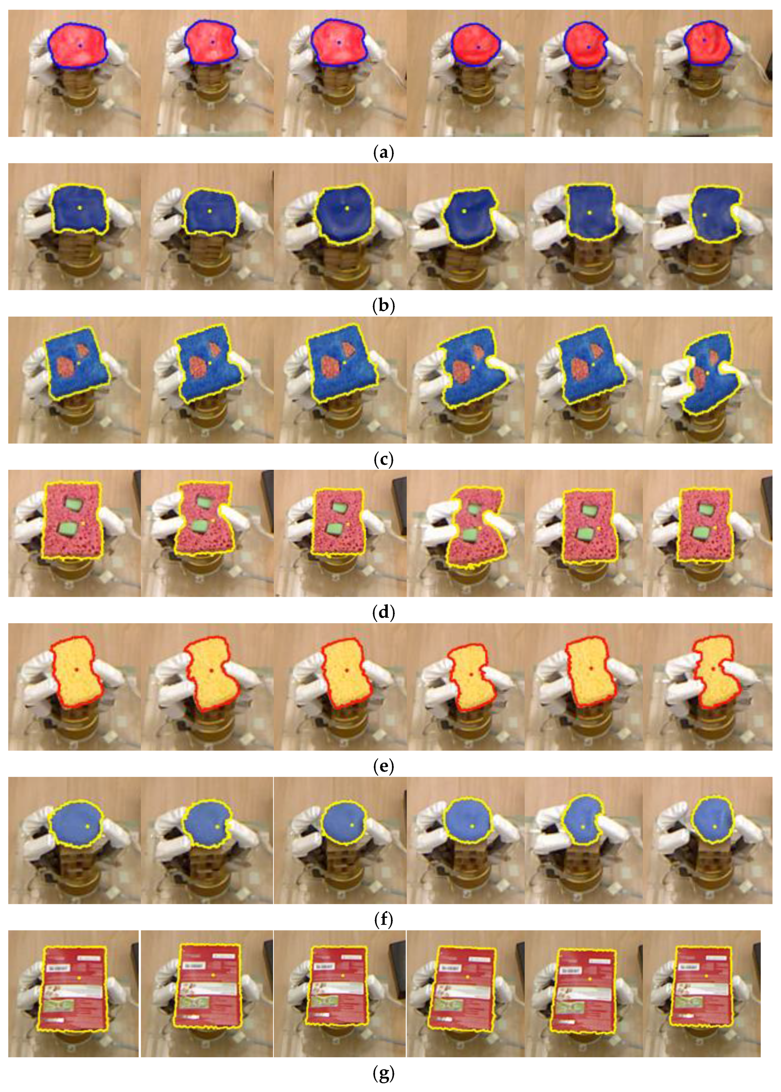
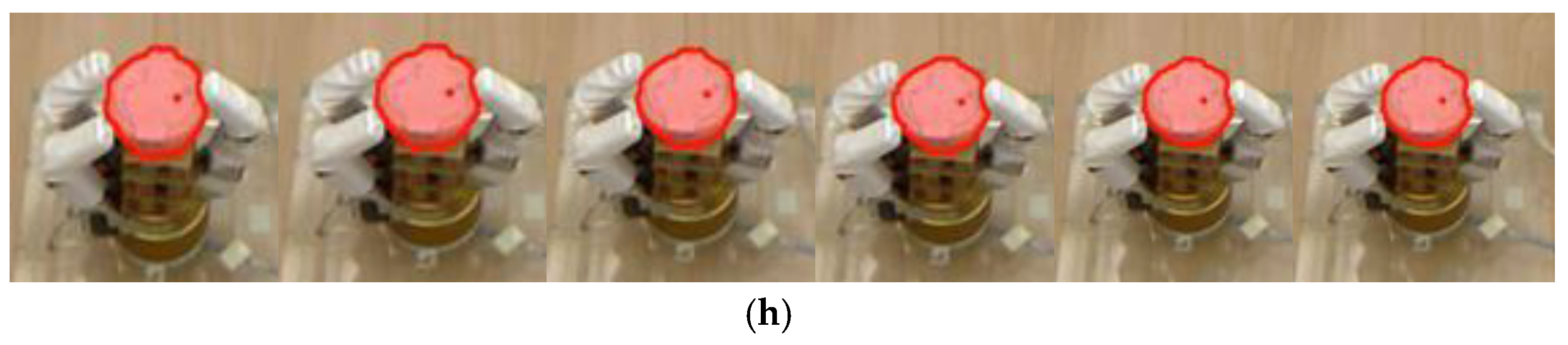
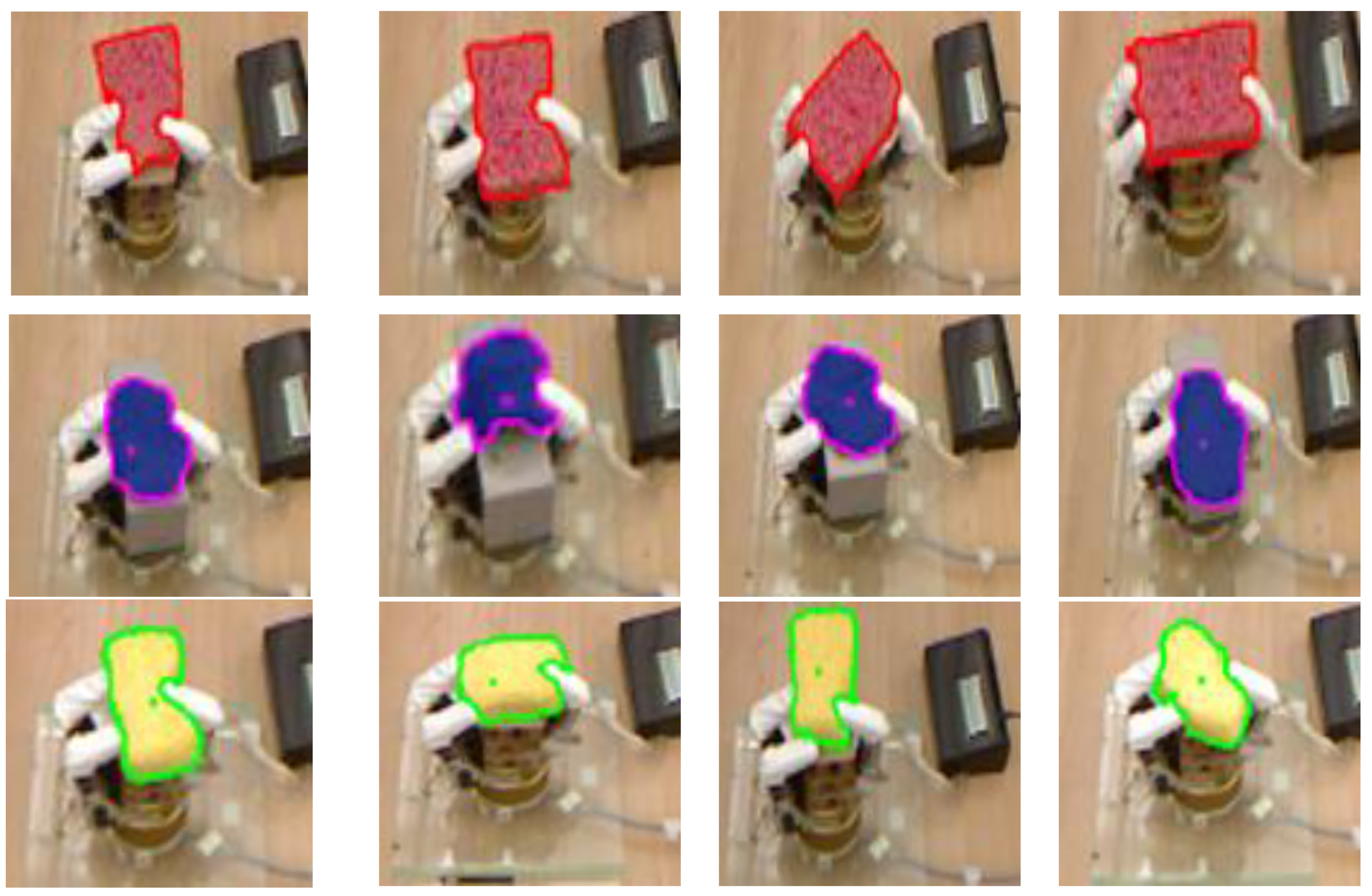
In order to characterize objects and classify them into different categories related to the material they are made of, and therefore recognize their deformation behavior, an automated measurement procedure is designed that uses a three-finger robotic Barrett hand. The hand applies a series of forces over predefined points distributed all around the object to be characterized, while the contour of the object is visually monitored with the solution described in the previous sections. The object contour obtained at different deformation stages using the fast level set method applied in the log-polar space is remapped into the RGB image coordinates, as shown in Figure 3d. A subset of the contours is then used to automatically identify the type of object the robot hand is manipulating. The original, not deformed, shape of the object does not influence the classification, and neither the choice of points over which force is applied. This is a benefit of the proposed method that monitors the relative deformation of the object only, while no formal model of the object is involved. Separate methods exist for optimal selection of contact points for the application of force to ensure stable grasp, and this aspect is beyond the scope of the present research.

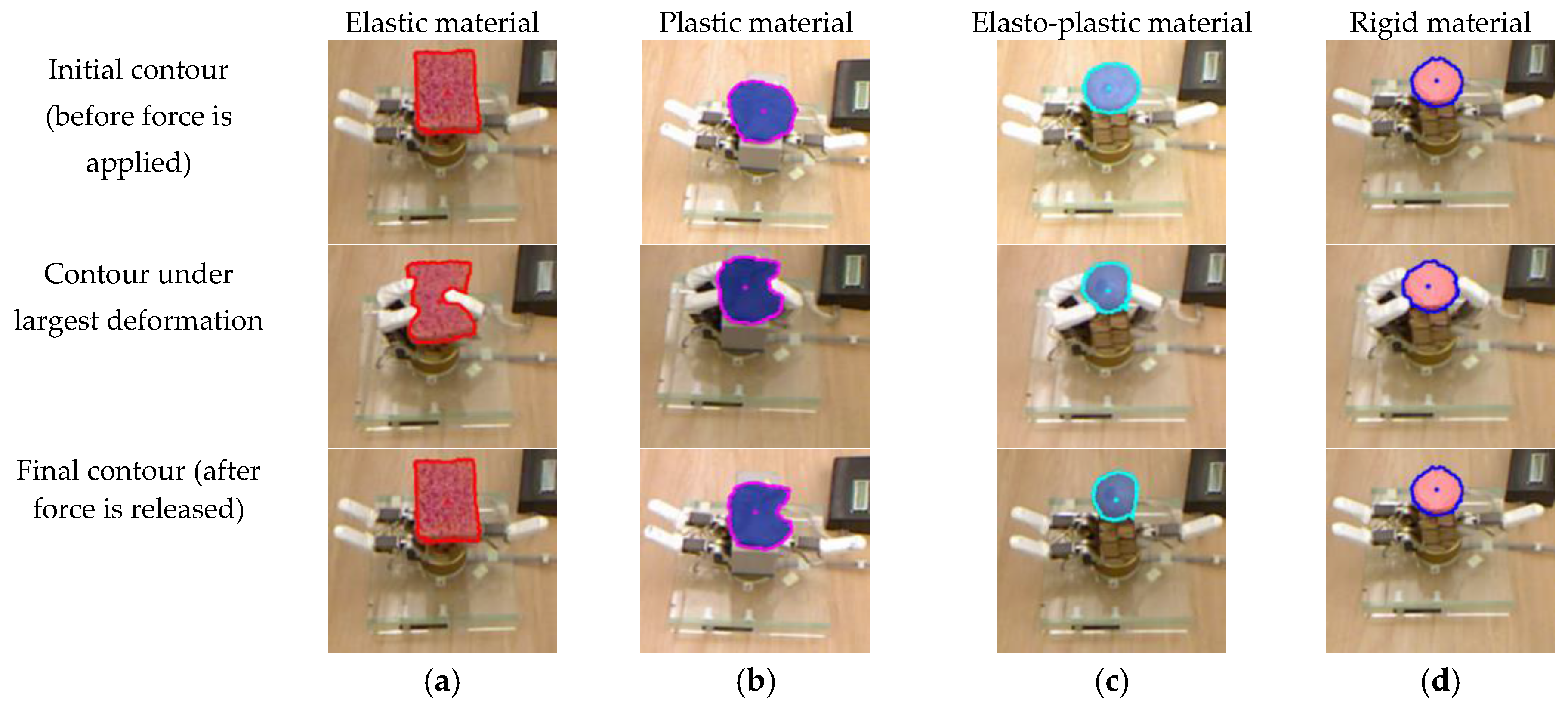
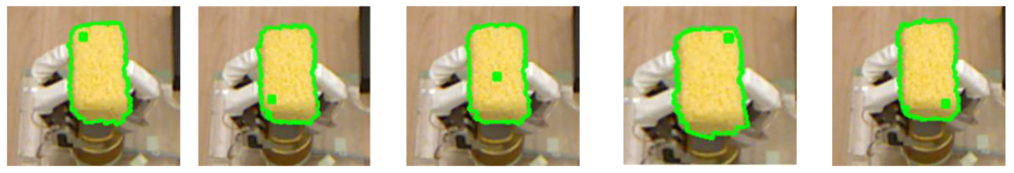
Elastic objects are known to return to their initial shape once the forces applied on them are released. Therefore, in order to detect if the object is elastic, the final deformation contour, after forces are removed, is compared to the initial deformation profile, collected in the beginning of the characterization procedure, that is before any force is applied, as well as to the contour obtained when the largest deformation takes place. If the initial and the final contours are almost identical, within a certain tolerated noise margin, and different from the contour under the largest deformation, the object is classified as elastic (Figure 5a).

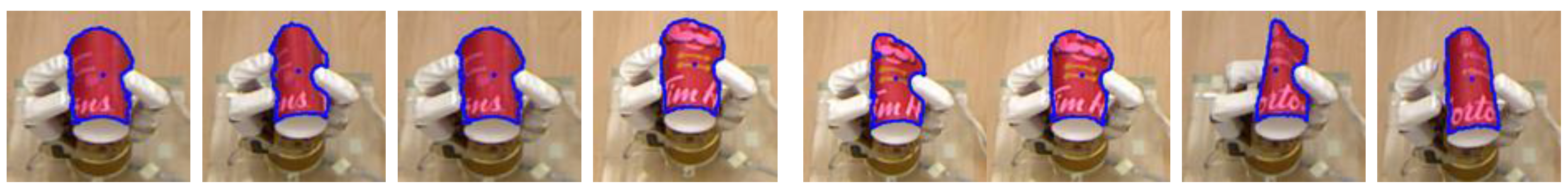
The comparison between the initial, largest deformation and final object contours is also exploited to detect plastic and elasto-plastic deformations. If these three contours are different, beyond a predefined tolerance of a few pixels in order to cope with the noise in the measurements, it means that either a plastic or an elasto-plastic behavior occurred. The differentiation between the plastic and elasto-plastic behaviors is achieved by comparing the final deformation contour with the contour under largest deformation. Given that an object made of plastic material memorizes the largest deformation experienced, if the final contour and the contour under largest deformation are almost identical, as shown in Figure 5b, it means that a plastic deformation occurred. On the other hand, elasto-plastic material has the property to partially, but not totally, recover from the deformation when the external force is released. This property is recognized by comparing again the final contour with the contour under largest deformation. If they are significantly different, as shown in Figure 5c, but not identical to the initial contour, then the material is considered to be one exhibiting elasto-plastic properties. Finally, if all three contours are identical, as shown in Figure 5d, the object is considered rigid, as no deformation is perceived by the contour tracking system under any amount of force.

In the current implementation, the three contours of interest (initial, largest deformation and final) are selected out of the sequence of contours under manual guidance to ensure proper evaluation of the classification algorithm. However, contour tracking also allows automatic extraction of these contours from the sequence. The frame prior to first deformation detection represents the initial contour; the frame in which the deformation changes direction is selected as the contour with largest deformation; and the frame after deformation stops is considered to be the final contour. Continuous contour tracking over the entire manipulation procedure also allows the detection of a special case of rigid objects that would break under the forces applied by the robot hand fingers. Close monitoring of the obtained contours in order to detect any abrupt changes, or definitive loss of contour, can be exploited to identify this sub-category of rigid objects.

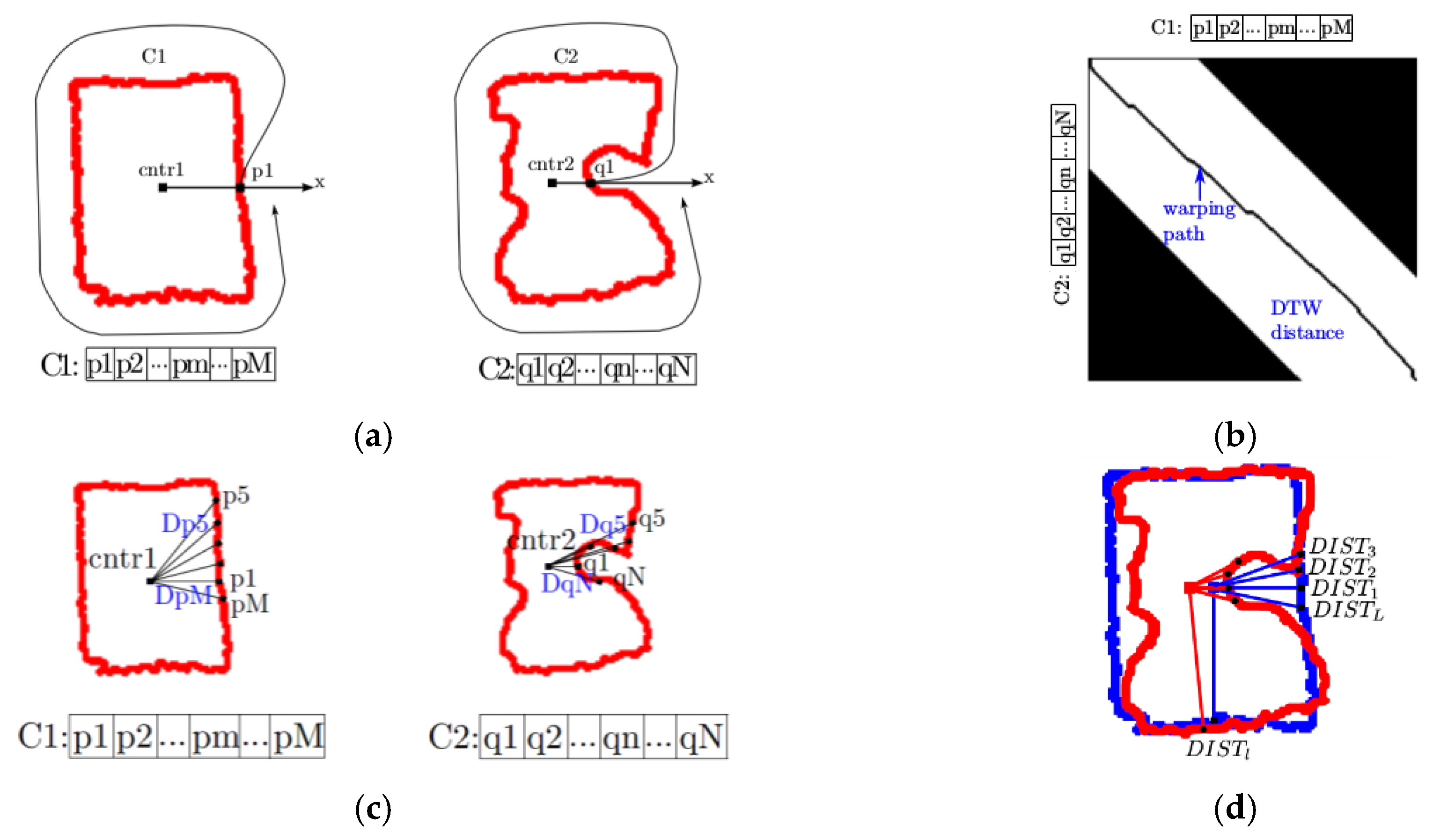
In order to perform the classification, the object contours are compared using dynamic time warping (DTW) to detect changes in the various stages of the object deformation. Dynamic time warping is a commonly used technique to align two sequences that may vary in length [21,39,40]. DTW is selected here because the number of pixels forming a contour can significantly vary in between successive frames, as a result of the deformation of the object. As such, DTW does not require extraction of features from the contours. It provides a robust distance-based method to compare contours of variable length, which also eliminates the need for explicit point-to-point matching of contour pixels or subsampling of the contours, and therefore allows full usage of the information available. In particular, starting from a contour, principal component analysis is applied to identify the center pixel of the contour, defined as follows [41]:

$$\mathit{c}\mathit{n}\mathit{t}\mathit{r}=\frac{{\sum }_{k=1}^K{\mathit{c}}_k}{K}$$

(7)

where $\mathit{c}\mathit{n}\mathit{t}\mathit{r}(x_{cntr}, y_{cntr})$ represents the center pixel of contour, $\tilde{C}$, the latter being composed of K pixels, ${\mathit{c}}_1, {\mathit{c}}_2,\dots , {\mathit{c}}_k(x_{c_k}, y_{c_k})$. The first pixel belonging to the contour (${\mathit{p}}_1$ in Figure 6a) is identified as being the pixel that satisfies the two conditions defined in Listing 4.

Listing 4. First pixel conditions

1: $\tan \frac{y_{\mathit{c}\mathit{n}\mathit{t}\mathit{r}}-y_{{\mathit{c}}_k}}{x_{\mathit{c}\mathit{n}\mathit{t}\mathit{r}}-x_{{\mathit{c}}_k}}=0$

2: ${\mathit{c}}_k$ is located on the right side of $\mathit{c}\mathit{n}\mathit{t}\mathit{r}$.

Listing 4. First pixel conditions

1: $\tan \frac{y_{\mathit{c}\mathit{n}\mathit{t}\mathit{r}}-y_{{\mathit{c}}_k}}{x_{\mathit{c}\mathit{n}\mathit{t}\mathit{r}}-x_{{\mathit{c}}_k}}=0$

2: ${\mathit{c}}_k$ is located on the right side of $\mathit{c}\mathit{n}\mathit{t}\mathit{r}$.

Once this pixel is identified, the contour sequence is filled up with the remaining contour pixels in the counterclockwise direction (along the arrow in Figure 6a).

Figure 6a shows an example of two consecutive contours $C_1={\mathit{p}}_1, {\mathit{p}}_2,\dots , {\mathit{p}}_m, \dots , {\mathit{p}}_M$ and $C_2= {\mathit{q}}_1, {\mathit{q}}_2,\dots , {\mathit{q}}_n, \dots , {\mathit{q}}_N$ at time $t$ and $t+1$, respectively. In order to compare the differences between $C_1$ and $C_2$, the local cost matrix, $d$, is used to evaluate the similarity of each pair of pixels in the sequences $C_1$ and $C_2$. In this matrix, each element $d[m,n]$ represents the Euclidean distance between the pixel ${\mathit{p}}_m$ from the first contour and the pixel ${\mathit{q}}_n$ from the second contour. The value of d[m,n] in the matrix is low (low cost) if ${\mathit{p}}_m$ and ${\mathit{q}}_n$ are similar to each other in their relative location, or high otherwise. The warping matrix is computed with an additional locality constraint [42]. This means that for the contour sequences $C_1$ and $C_2$, instead of calculating the DTW distance over all pairs of pixels, the DTW distance is only calculated for the part of warping matrix where the condition $\left|M-N\right|\le v$ is satisfied. With this locality constraint, the computed DTW distance is restricted to a band (shown in white in Figure 6b), along the diagonal of the warping matrix, which speeds up the DTW distance calculation. As such, in Figure 6b, the black areas are eliminated from the calculations in order to accelerate the computation time. The DTW algorithm with locality constraint is summarized in Algorithm 3:

Algorithm 3. Conditional DTW algorithm with locality constraint.

Input:

$C_1={\mathit{p}}_1, {\mathit{p}}_2,\dots , {\mathit{p}}_m,\dots , {\mathit{p}}_M$ : Sequence of length $M$;

$C_2={\mathit{q}}_1, {\mathit{q}}_2,\dots , {\mathit{q}}_n,\dots , {\mathit{q}}_N$ : Sequence of length $N$.

Output:

DTW matrix

1: DTW = matrix [M+1, N+1];

2: v = 1/5×max(M, N)

3: v = max(v, |M − N |)

4: for m do = 0 : M

5:      for n do = 0 : N

6:          DTW[m,n] = ∞

7:      end for

8: end for

9: DTW[0, 0] = 0

10: for m = 1 : M do

11:      for n = max(1, m-v) : min(N, m+v) do

12:          DTW[m,n] = d[m, n] + min$\{\begin{array}{c}\mathrm{DTW}[\mathrm{i}-1, \mathrm{j}]\\ \mathrm{DTW}[\mathrm{i}, \mathrm{j}-1]\\ \mathrm{DTW}[\mathrm{i}-1, \mathrm{j}-1]\end{array}$

13:      end for

14: end for

15: return DTW[M, N]

The optimal warping path $W=w_1,w_2,\dots ,w_l,\dots ,w_L$, with $w_l=(m_l, n_l),$ is the one with the minimal overall cost from the DTW matrix, where $max(M, N)\le L<(M+N)$, and L is the length of the warping path. This warping path must satisfy the three conditions defined in Listing 5.

Listing 5. Warping path conditions

1: Boundary condition: $w_1$= (1, 1) and $w_L$ = (M, N);

2: Monotonicity condition: $m_1\le m_2\le \dots \le m_L$ and $n_1\le n_2\le \dots \le n_L$;

3: Step size condition: $w_{l+1}-w_l\in \left\{(1,0),(0,1),(1,1)\right\}$ for $l\in [1, L-1].$

Listing 5. Warping path conditions

1: Boundary condition: $w_1$= (1, 1) and $w_L$ = (M, N);

2: Monotonicity condition: $m_1\le m_2\le \dots \le m_L$ and $n_1\le n_2\le \dots \le n_L$;

3: Step size condition: $w_{l+1}-w_l\in \left\{(1,0),(0,1),(1,1)\right\}$ for $l\in [1, L-1].$

It is computed in reverse order of the indices starting with $w_L=(M, N)$. Once $w_l=(m, n)$ is calculated, the next elements are defined using the following equation [39]:

$$w_{l-1}=\{\begin{array}{c}(1, \mathrm{n}-1), \mathrm{if} \mathrm{m}=1\\ (\mathrm{m}-1, 1), \mathrm{if} \mathrm{n}=1\\ \mathrm{argmin}\left\{\mathrm{DTW}(\mathrm{m}-1, \mathrm{n}-1), \mathrm{DTW}(\mathrm{m}-1, \mathrm{n}), \mathrm{DTW}(\mathrm{m}, \mathrm{n}-1)\right\}, \mathrm{otherwise}\end{array}$$

(8)

With the above three warping path conditions, the warping path matches the two contour sequences $C_1$ and $C_2$ by assigning the pixel ${\mathit{p}}_m$ of $C_1$ to the pixel ${\mathit{q}}_n$ of $C_2$ so that an element $w_l$ of the warping path stands for a pair of pixels (${\mathit{p}}_m$, ${\mathit{q}}_n$). The optimal path is shown as a black line over the white band in Figure 6b.

In order to compute the differences between the initial contour, $b{w}_0$, the contour under largest deformation, $b{w}_1$, and the contour after the force is removed, $b{w}_2$, we compute a score inspired from [42]. However, in our case the score is made more robust as it also takes into account shifting and slight rotation movements that the object could exhibit during manipulation. The proposed score is calculated as:

$$score(C_1, C_2)=e^{-\frac{{\sum }_{l=1}^{L}DIS{T}_l}{L}}$$

(9)

where L is the length of the warping path, and $DIS{T}_l=|D{p}_l-D{q}_l|$ with $D{p}_l$ the Euclidean distance between the pixel ${\mathit{p}}_m$ and its contour center $\mathit{c}\mathit{n}\mathit{t}{\mathit{r}}_1$, or $D{p}_l=\left|\right|{\mathit{p}}_m-\mathit{c}\mathit{n}\mathit{t}{\mathit{r}}_1\left|\right|$, and $D{q}_l$ is the Euclidean distance between the pixel ${\mathit{q}}_n$ and its contour centre $\mathit{c}\mathit{n}\mathit{t}{\mathit{r}}_2$, or $D{q}_l=\left|\right|{\mathit{q}}_n-\mathit{c}\mathit{n}\mathit{t}{\mathit{r}}_2\left|\right|.$ Figure 6c illustrates the Euclidean distances between a pixel and the center of the contour for the two contours considered previously. However, because it is desired that the method is robust to noise and fast at the same time, we impose two conditions in order to consider that a contour has been deformed. In particular, we verify if a displacement of the contour occurred and that the displacement affects more than three contiguous pixels over the contour. Considering the sequence of $DIS{T}_l$ values, if the value of an element in this vector is larger than a threshold (e.g., 4 pixels in our work), it is considered that a movement occurred at that location on the contour, otherwise, the difference is attributed to noise and it is considered that no movement occurred. In case the contour has moved, we also verify the number of contiguous pixels affected by the movement. In particular, if the number of contiguous pixels with movement is larger than 3 pixels, the contour is considered being deformed. An example is shown Figure 6d. The blue contour represents the contour at time t, and the red one is the contour at time t + 1. The pairs of pixels $({\mathit{p}}_1, {\mathit{q}}_1), ({\mathit{p}}_2, {\mathit{q}}_2), ({\mathit{p}}_3, {\mathit{q}}_3), ({\mathit{p}}_m, {\mathit{q}}_n)$ and $({\mathit{p}}_M, {\mathit{p}}_N)$ from these two contours, respectively, are matched by the DTW algorithm. $DIS{T}_l$ is the distance between two pixels ${\mathit{p}}_m$ and ${\mathit{q}}_n$ and its value is smaller than 4. Therefore there is no movement at pixel ${\mathit{p}}_m$. $DIS{T}_1$ is the distance between pixels ${\mathit{p}}_1$ and ${\mathit{q}}_1$ and its value is larger than 4 so that pixel ${\mathit{p}}_1$ is in movement. The same thing can be noticed for $DIS{T}_2, DIS{T}_3$ and $DIS{T}_L$, meaning that the pixels ${\mathit{p}}_2, {\mathit{p}}_3$and ${\mathit{p}}_L$ are in movement as well. As four contiguous pixels have movement, it is considered that the contour at the pixels ${\mathit{p}}_L$, ${\mathit{p}}_1$, ${\mathit{p}}_2$ and ${\mathit{p}}_3$ is deformed. Only the deformed contours are evaluated using Equation (9).

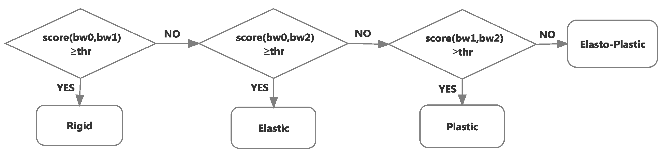
If the contour is deformed, based on the scores computed pairwise between the initial contour, $b{w}_0$, the contour under largest deformation, $b{w}_1$, and the final contour after the force is removed, $b{w}_2$, using Equation (9), the decision process for classifying the object as rigid, elastic, plastic or elasto-plastic is illustrated in Figure 7. The value of the threshold thr applied on the score was empirically set to 0.75. Experiments revealed that for larger threshold values (e.g., thr = 1.0), the proposed classification approach is over sensitive and noise impacts the classification; on the other hand, for lower threshold values (e.g., thr = 0.5), the approach is insufficiently responsive to slightly different contours.

4. Experimental Results

The proposed approach is tested on 9 objects with material properties belonging to 4 categories, as illustrated in the first row of Figure 5, to evaluate the performance of the framework. An investigation was initially performed to study the impact of the various parameters of the proposed approach. It is worth noting that once the internal parameters have been set, as reported in the paper, no further tuning was performed. All experiments were conducted with the same parameters, independently of the object material, shape of object, location of the Kinect sensor, and amount of force applied. This demonstrates the robustness of the proposed approach.

The tests performed reveal that the minimal distance of the Kinect sensor with respect to the surface of the object for which the contour can be reliably extracted and tracked is around 50 cm (Figure 8a). The contour can be tracked up to 150 cm separating the Kinect sensor from the object. However, the best range of distances to perform contour tracking is between 55 and 75 cm, given the resolution of the Kinect sensor. The relative sensor-to-object distance has however an impact on the performance of the classification, because a larger distance produces fewer details over the contour given that the object of interest appears smaller in the image. As a result, when only light forces are applied on the object, the deformation is smaller and may be insufficient in magnitude to be perceived from contour tracking over the color image. The tests reported in this paper are performed at a 55 cm distance, for various positions and orientations of the Kinect sensor around the object, as shown in Figure 8b. Experiments are also conducted for various initial positions and orientations of the object within the robot hand (Figure 9), and for various grasping forces, in order to evaluate the robustness of the solution with respect to all these factors.

Figure 9 shows several testing cases for objects with different shape and color properties and under various starting conditions where the object is initially grabbed in different ways by the robot hand. These results illustrate that the contour of the deformed object is correctly detected and tracked throughout the manipulation regardless of the initial position or orientation of the object in the robot hand, and under several magnitudes of applied force and levels of deformation. It can be noticed that the robot hand fingers are covered with white rubber gloves. This proved useful for several reasons, including the protection of the sensible touch sensors mounted (but not used in this work) on the robot hand, to ensure the uniformity of color over the entire surface of the fingers, and making them sufficiently contrasting to the background surface and objects.

Figure 10 illustrates testing scenarios where contour tracking is successfully achieved with various materials, shapes and textures. Objects with various textures and inserts of different color and material were tested, as shown in Figure 10c, d, g, to confirm that the contour tracking is not distracted by colors or lighting effects, and that the level sets applied in the log-polar domain perform reliably under more challenging situations. It can be observed that the solution tracks only the outside contour and does not capture the internal details of the objects at any stage.

Figure 11 shows that the contour is also correctly tracked regardless of the position of the Kinect sensor with respect to the object (see as well Figure 8b). Experimentation also revealed that for a distance of 55 cm from the Kinect to the object, the tolerance to shifting movements of the object during manipulation is of about 0.7 cm in any direction, and the rotation of the object as a result of the manipulation that is tolerated is about 4° in order not to impede on the classification performance. This results from the fact that no registration of the object or contour is performed in between the three contours that are compared with the DTW technique. However, the contour tracking process itself is much more robust to translations and rotations of the object.

Figure 12 demonstrates that the solution is also relatively robust to the location of the user-selected fixation point, marked by a green dot. One can notice that a more central position of the 2D fixation point leads to a smoother contour, while the contour is more jagged if the user selected point is closer to the sides of the object. This is a consequence of the use of a log-polar mapping which centers the contour extraction on the selected fixation point.

To evaluate the object material characterization with the proposed dynamic time warping approach, tests are repeated 60 times over nine objects (i.e., 3 plastic, 3 elastic, 1 elasto-plastic and 2 rigid). During each repetition, the object is compressed by the robot hand on three contact points distributed over its contour. A light, medium or strong force is respectively applied and then released. The confusion tables for the three possible strengths of grasping forces are shown in Figure 13. These confusion tables map the detected category of an object against the target category, here considered as ground truth from the a priori knowledge that we have of each object. Confusion tables highlight correct classifications (green cells) and misclassification cases (red cells), and allow for the calculation of average success (green writing) and failure (red writing) rates, by category and overall (blue cells), under specific testing conditions, here related to the magnitude of the applied force.

An overall recognition rate of 69.8% over all material types is obtained when a light grasping force is applied, of 98.3% for a medium force, and of 98.3% for a strong force. These results are coherent with our expectations because light forces result in relatively small contour deformations. Moreover, due to the relatively low accuracy of the Kinect sensor, tiny movements cannot be perceived, leading overall to a lower classification performance under light forces. On the other hand, as the magnitude of force applied by each finger increases, under the medium and strong forces categories, the resulting deformation magnitude easily reaches within the detectable range for the Kinect sensor image resolution, and the contour tracker performs significantly better. This demonstrates the need to apply sufficiently large forces while attempting to characterize a deformable object.

In terms of material types, an overall recognition rate (over all magnitudes of force) of 99.4% is achieved for elastic material (average of E columns in Figure 13, 71.9% for plastic material (average of P columns), 85.6% for elasto-plastic material (average of EP columns), and 100% for rigid material (average of R columns). These results show that the approach works very well for most types of object material, but remains more limited for plastic materials, especially if light forces are considered. Elastic material is in very few cases (i.e., 3 out of 180 samples or 1.7% of cases) confused with a rigid material, but only when light grasping forces are applied, which creates insufficient displacement of the contour. The lower performance for plastic material is related to the use of plasticine packed in a transparent plastic wrap as sample of plastic objects, which is in fact not a perfectly plastic material. Moreover, the robot fingers tend to stick to the plasticine dough, especially when medium and strong forces are applied, impacting on the contour tracking and category recognition. As one can observe in column P of the table for light forces, Figure 13a, only a few samples are correctly identified as being of plastic material (25.6%) when a light force is applied, while 95% of the plastic samples are properly classified under medium and strong force application. The classification performance is significantly improved under medium and strong forces compared with the light force case, as plastic material tends to be confused with elasto-plastic, elastic, or even rigid material when insufficient force is applied to significantly deform it. For elasto-plastic material (columns EP in Figure 13), the percentage of correctly classified samples varies from 56.7% under a light force, to 100% under medium or strong force, which is coherent with the previous observation that sufficient force needs be applied to properly characterize a deformable object composed of any material. Elasto-plastic material is confused with elastic material when insufficient force is applied to reach a partially remaining deformation. Finally, rigid objects (columns R in Figure 13) obtain a very high recognition rate regardless of the magnitude of force applied on them. This is essentially due to the simplicity of their recognition, which relies on no significant deformation occurring under no circumstances. Given that the proposed approach mainly aims at recognizing the type of material the objects are made of, rather than generate formal models, the original shape of the object does not influence the procedure, for the reasons provided in Section 3.3.

Figure 14 shows an example of a more complex scenario involving an object composed of material that exhibits multiple deformation stages, and therefore belongs to different categories at various stages of deformation. Under light forces, the object, consisting of a cardboard cup, exhibits an elastic behavior (images 1 to 3 in Figure 14), under medium forces and up to a certain limit the object remains in its elastic stage, and then transfers to the elasto-plastic stage (images 4 to 7 in Figure 14). Finally, when a larger force is applied, the object further transitions from the elasto-plastic to its plastic stage (image 8 in Figure 14). In spite of the complex behavior of such an object, the performance of the proposed contour tracker and deformable object classification remains consistent with the results reported for elastic, elasto-plastic, and for plastic materials in Figure 13.

In the proposed tracking and classification system, the RGB image and the point cloud are collected directly from the Kinect sensor with a frame rate of 30 Hz. The processing is performed off-line after the sequence of RGB-D data is recorded. For each frame, the average contour tracking time is 44.4 ms. The average classification time is 35.2 ms when the three relevant contours are analyzed by the classification system, as detailed in Figure 7. The experiments are carried out on a 2.6 GHz Intel Core i7 with 8 GB of RAM laptop. Figure 15 and Figure 16 present the respective tracking time per frame and classification time per object. The presented computation time corresponds to the average process duration, in ms, over the 60 trials performed on each object and over all objects belonging to the same category of material, or being submitted to the same magnitude of force (light, medium, strong).

Figure 15a and Figure 16a show that both the contour tracking and classification time remain in the same range under various magnitudes of force applied to generate the deformation, with light forces leading to slightly faster results due to very tiny deformations that occur. On the other hand, it is noticeable in Figure 15b that the contour tracking process for elastic and rigid objects can take slightly longer. For elastic objects, this difference is explained by the fact that elastic material exhibits the most significant deformation over the manipulation process, going from the original smooth contour to a significantly deformed shape at largest deformation, and then back to the original shape, as exemplified in Figure 10c,e. For rigid objects, the average result reported in Figure 15b is impacted by the larger and heavily textured rigid object shown in Figure 10g. In this case, contour tracking takes on average 80 ms, while for the simpler rigid object in Figure 10h, contour tracking is achieved in about 40 ms. For plastic objects where the contour only moves toward the interior of the object, the level sets procedure requires fewer tracking steps to capture the whole deformation process.

Regarding classification computation time, some differences are observed in between testing cases. Objects probed with only a light force often do not exhibit deformations that are large enough to support proper classification, as was demonstrated in Figure 13a. The classification process is typically faster but the accuracy is also impacted. On the other hand, while it may appear that classifying elastic or rigid objects takes about 10 ms more than recognizing plastic or elasto-plastic ones, a close analysis reveals that the classification time is also influenced by the relative size that the object of interest occupies in the processed RGB images, similar to what impacted contour tracking on those objects. Items shown in Figure 10c,e (elastic), and Figure 10g (rigid) are larger in the image than the other objects, independently of their material characteristics. These visually larger objects generate contours with a larger number of points. Therefore, the DTW process (Algorithm 3) must establish correspondence and estimate distances on a larger number of points to identify a longer, L, warping path. This explains why the average classification time for elastic (42 ms) and rigid (38 ms) objects are overall slightly longer than for plastic (28 ms) or elasto-plastic (29 ms) objects, among the set of test cases examined in this study.

Overall, the contour tracking process supports an update rate of up to 23 Hz, without code optimization. While this is slightly slower than the available acquisition framerate of 30 Hz from the Kinect sensor, it compares with the performance reported by other researchers who applied level sets on color images [43]. Moreover, the robotic hand moves relatively slowly while performing the object probing, with the closing and reopening of the fingers, while in touch with the object, taking on average 2 s. The achieved contour tracking speed therefore proves sufficient to handle the probing process that takes place at about 0.5 Hz. Also, this overall procedure is meant to operate as an off-line object characterization process taking place before the actual manipulation happens. Therefore, real-time processing is not an absolute requirement for deformable object characterization.

5. Conclusions

The paper proposes a robust approach for non-rigid object deformation tracking in RGB-D data with the purpose of characterizing the material that deformable objects are made of with the assistance of a robotic hand. The approach advantageously integrates well-established techniques for background removal and distance-based clustering from RGB-D data with an original application of the fast level set method in the log-polar domain in order to detect and track the contour of an object of interest in the RGB-D data stream while it is manipulated by a robot. Dynamic time warping is employed with a modified scoring scheme to characterize the object’s material properties based on contour extracted at strategic stages of the manipulation by the robot hand. The proposed scoring scheme provides tolerance to translations and rotations that the object may exhibit, beyond its deformation, as a consequence of the manipulation. The proposed solution achieves an average classification rate over all material types of 98.3% when a strong force is applied on the object and of 88.8% regardless of the force magnitude, while supporting an update rate of 23 Hz. The main contributions of this research consists of an original use of a log-polar map encoded in the YUV color space to actively track contours with the fast level set method and to refine its performance. It also introduces a classification scheme that provides accurate material recognition while tolerating object shifts and rotations. It represents a first attempt to apply these concepts to the complex case of visual deformation tracking and robust classification of the physical behavior of non-rigid objects undergoing robotic manipulation.

References

1. Saadat, M.; Nan, P. Industrial applications of automatic manipulation of flexible materials. Int. J. Ind. Robots 2012, 29, 434–442. [Google Scholar] [CrossRef]
2. Ono, E. Automated Swing System and Unfolding Fabric; Robot Manipulation of Deformable Objects; Henrich, D., Worn, H., Eds.; Springer: London, UK, 2000. [Google Scholar]
3. Houachine, N.; Dequidt, J.; Berger, M.O.; Cotin, S. Single view augmentation of 3D elastic objects. In Proceedings of the IEEE International Symposium on Mixed and Augmented Reality, Munich, Germany, 10–12 September 2014; pp. 229–236.
4. Krainin, M.; Henry, P.; Ren, X.; Fox, D. Manipulator and object tracking for in-hand 3D object modeling. Int. J. Robot. Res. 2011, 30, 1311–1327. [Google Scholar] [CrossRef]
5. Petit, A.; Lippiello, V.; Siciliano, B. Real-time tracking of 3D elastic objects with an RGB-D sensor. In Proceedings of the IEEE International Conference on Intelligent Robots and Systems, Hamburg, Germany, 28 September–3 October 2015; pp. 3914–3921.
6. Zaidi, L.; Bouzgarrou, B.; Sabourin, L.; Menzouar, Y. Interaction modeling in the grasping and manipulation of 3D deformable objects. In Proceedings of the IEEE International Conference on Advanced Robotics, Istanbul, Turkey, 27–31 July 2015; pp. 504–509.
7. Stuckler, J.; Behnke, S. Perception of deformable objects and compliant manipulation for service robots. In Soft Robotics; Verl, A., Albu-Schäffer, A., Brock, O., Raatz, A., Eds.; Springer: Berlin Heidelberg, Germany, 2015; pp. 69–80. [Google Scholar]
8. Khalil, F.F.; Payeur, P. Dexterous robotic manipulation of deformable objects with multi-sensory feedback—A review. In Robot Manipulators, Trends and Development; Jimenez, A., Al Hadithi, B.M., Eds.; In-Tech: Vukovar, Croatia, 2010; pp. 587–619. [Google Scholar]
9. Cretu, A.M.; Payeur, P.; Petriu, E.M. Soft object deformation monitoring and learning for model-based robotic hand manipulation. IEEE Trans. Syst. Man Cybern. Part B 2012, 42, 740–753. [Google Scholar] [CrossRef] [PubMed]
10. Mateo, C.M.; Gil, P.; Mira, D.; Torres, F. Analysis of shapes to measure surfaces. In Proceedings of the IEEE Conf. Informatics in Control, Automation and Robotics, Colmar, Alsace, France, 21–23 July 2015; pp. 60–65.
11. Elbrechter, C.; Haschke, R.; Ritter, H. Folding paper with anthropomorphic robot hands using real-time physics-based modeling. In Proceedings of the IEEE International Conference on Humanoid Robots, Osaka, Japan, 29 November–1 December 2012; pp. 210–215.
12. Frank, B.; Schmedding, R.; Stachniss, C.; Teschner, M.; Burgard, W. Learning the elasticity parameters of deformable objects with a manipulation robot. In Proceedings of the IEEE International Conference on Intelligent Robots and Systems, Taipei, Taiwan, 18–22 October 2010; pp. 1877–1883.
13. Schulman, J.; Lee, A.; Ho, J.; Abbeel, P. Tracking deformable objects with point clouds. In Proceedings of the IEEE International Conference on Robotics and Automation, Karlsruhe, Germany, 6–10 May 2013.
14. Boonvisut, P.; Çavusoglu, M.C. Identification and active exploration of deformable object boundary constraints through robotic manipulation. Int. J. Robot. Res. 2014, 22, 1446–1461. [Google Scholar] [CrossRef] [PubMed]
15. Zollhöfer, M.; Nieβner, M.; Izadi, S.; Rehmann, C.; Zach, C.; Fisher, M.; Wu, C.; Fitzgibbon, A.; Loop, C.; Theobalt, C.; et al. Real-time non-rigid reconstruction using an RGB-D camera. ACM Trans. Graph. 2014, 33, 156. [Google Scholar] [CrossRef]
16. Foresti, G.L.; Pellegrino, F.A. Automatic visual recognition of deformable objects for grasping and manipulation. IEEE Trans. Syst. Man Cybern. Appl. Rev. 2004, 34, 325–333. [Google Scholar] [CrossRef]
17. Fischler, M.A.; Bolles, R.C. Random sample consensus: A paradigm for model fitting with applications to image analysis and automated cartography. Commun. ACM 1981, 24, 381–395. [Google Scholar] [CrossRef]
18. Sproull, R.F. Refinements to nearest-neighbor searching in k-dimensional trees. Algorithmica 1991, 6, 579–589. [Google Scholar] [CrossRef]
19. Traver, V.J.; Pla, F. Log-polar mapping template design: From task-level requirements to geometry parameters. Image Vis. Comput. 2008, 26, 58–74. [Google Scholar] [CrossRef]
20. Shi, Y.; Karl, W.C. A real-time algorithm for the approximation of level-set-based curve evolution. IEEE Trans. Image Process. 2008, 17, 645–656. [Google Scholar] [PubMed]
21. Romero, J.; Kragic, D.; Kyrki, V.; Argyros, A. Dynamic time warping for binocular hand tracking and Reconstruction. In Proceedings of the IEEE International Conference on Robotics and Automation, Pasadena, CA, USA, 19–23 May 2008; pp. 2289–2294.
22. Mateo, C.M.; Gil, P.; Torres, F. 3D visual data-driven spatiotemporal deformations for non-rigid object grasping using robot hands. Sensors 2016, 16, 640. [Google Scholar] [CrossRef] [PubMed]
23. Choi, M.-H.; Wilber, S.C.; Hong, M. Estimating material properties of deformable objects by considering global object behavior in video streams. Multimedia Tools Appl. 2015, 74, 3361–3375. [Google Scholar] [CrossRef]
24. Kraft, D.; Pugeault, N.; Baseski, E.; Popovic, M.; Kragic, D.; Kalkan, S.; Worgotter, F.; Kruger, N. Birth of the object: Detection of objectness and extraction of object shape through object-action complexes. Int. J. Humanoid Robot. 2008, 5, 247–265. [Google Scholar] [CrossRef]
25. Navarro-Alarcon, D.; Yip, H.M.; Wang, Z.; Liu, Y.-H.; Zhong, F.; Zhang, T.; Li, P. Automatic 3-D manipulation of soft object by robotic arms with an adaptive deformation model. IEEE Trans. Robot. 2016, 32, 429–441. [Google Scholar] [CrossRef]
26. Hur, J.; Lim, H.; Ahn, S.C. 3D deformable spatial pyramid for dense 3D motion flow of deformable object. In Proceedings of the ISVC2014, Las Vegas, NV, USA, 8–10 December 2014; pp. 118–127.
27. Mishra, A.K.; Aloimonos, Y. Active segmentation. Int. J. Humanoid Robot. 2009, 6, 361–386. [Google Scholar] [CrossRef] [PubMed]
28. Macknojia, R.; Chavez-Aragon, A.; Payeur, P.; Laganière, R. Calibration of a network of Kinect sensors for robotic inspection over a large workspace. In Proceedings of the IEEE Workshop on Robot Vision, Tampa, FL, USA, 15–17 January 2013; pp. 184–190.
29. Rusu, R.B. Semantic 3D Object Maps for Everyday Manipulation in Human Living Environments. Ph.D. Thesis, Technische Universität München, Münche, Germany, 2009; pp. 86–88. [Google Scholar]
30. The Point Cloud Library (PCL). Available online: http://pointclouds.org/ (accessed on 15 March 2017).
31. Chessa, M.; Solari, F. Local Feature Extraction in Log-Polar Images; Springer International Publishing: Cham, Switzerland, 2015; Volume 9279, pp. 410–420. [Google Scholar]
32. Chen, Y.; Rui, Y.; Huang, T.S. JPDAF based HMM for real-time contour tracking. In Proceedings of the IEEE Computer Society Conference on Computer Vision and Pattern Recognition, Kauai, HI, USA, 8–14 December 2001; Volume 1, pp. 543–550.
33. Xu, C.; Pham, C.D.; Prince, J.I. Handbook of Medical Imaging, Volume 2. Medical Image Processing and Analysis; Chapter 3: Image Segmentation Using Deformable Models; SPIE Press: Bellingham, WA, USA, 2000; pp. 129–174. [Google Scholar]
34. Sonka, M.; Hlavac, V.; Boyle, R. Image Processing, Analysis, and Machine Vision; Brooke/Cole Publishing Company: Pacific Grove, CA, USA, 2008. [Google Scholar]
35. Angelini, E.; Jin, Y.; Laine, A. Handbook of Biomedical Image Analysis; Wilson, D., Laxminarayan, S., Eds.; Volume 3: Registration Models; Chapter 3: State of the Art of Level Set Methods in Segmentation and Registration of Medical Imaging Modalities; Springer: New York, NY, USA, 2005; pp. 47–101. [Google Scholar]
36. Mishra, A.; Aloimonos, Y.; Fah, C.L. Active segmentation with fixation. In Proceedings of the IEEE International Conference on Computer Vision, Kyoto, Japan, 27 September–4 October 2009; pp. 468–475.
37. Thida, M.; Chan, K.L.; Eng, H.-L. An improved real-time contour tracking. In Proceedings of the Pacific-Rim Symposium on Image and Video Technology, Hsinchu, Taiwan, 11–13 December 2006; pp. 702–711.
38. Chan, T.; Vese, L.A. Active contours without edges. IEEE Trans. Image Process. 2001, 10, 266–277. [Google Scholar] [CrossRef] [PubMed]
39. Muller, M. Information Retrieval for Music and Motion; Springer: Berlin Heidelberg, Germany, 2007. [Google Scholar]
40. Adwan, S. Reviews, Refinements and New Ideas in Face Recognition; Chapter 12: Robust Face Detection through Eyes Localization Using Dynamic Time Warping Algorithm; InTech: Rijeka, Croatia, 2011; pp. 249–270. [Google Scholar]
41. Smith, L.I. A Tutorial on Principal Components Analysis: Introduction. Available online: http://www.cs.otago.ac.nz/cosc453/student tutorials/principal components.pdf (accessed on 15 March 2017).
42. Gonzalez-Sosa, E.; Vera-Rodriguez, R.; Fierrez, J.; Ortega-Garcia, J. Comparison of body shape descriptors for biometric recognition using MMW images. In Proceedings of the 22nd International Conference on Pattern Recognition, Stockholm, Sweden, 24–28 August 2014; pp. 124–129.
43. Bibby, C.; Reid, I. Real-time tracking of multiple occluding objects using level sets. In Proceedings of the IEEE International Conference on Computer Vision and Pattern Recognition, Istanbul, Turkey, 23–26 August 2010; pp. 1307–1314.
Figure 1. Framework for object detection, contour tracking and material classification from RGB-D data.
Robotics 06 00005 g001
Figure 2. (a) Raw point cloud from Kinect with registered color information; (b) table extraction result; and (c) identified cluster representing the object of interest.
Robotics 06 00005 g002
Figure 3. (a) Cartesian to log-polar domain transformation; (b) RGB image (187 × 200 pixels) corresponding to the area of interest extracted from the point cloud shown in Figure 2a with 2D fixation point shown in green; (c) log-polar image (93 × 167 pixels) corresponding to the RGB image and initial contour shown in green; and (d) RGB image with Cartesian contour (187 × 200 pixels) obtained by inverse mapping from the log-polar image.
Robotics 06 00005 g003
Figure 4. (a) Representation of the curve C ˜ , and the two lists of neighboring pixels L ˜ i n and L ˜ o u t in the log-polar domain; (b) The motion of switching pixels between L ˜ i n and L ˜ o u t ; (c) Representation of the 4-connected discrete neighborhood, N 4 ˜ ( x ) , of a pixel x . Each element of the grid denotes a pixel of the image.
Robotics 06 00005 g004
Figure 5. Contour tracking comparison for objects made of material with various properties: (a) elastic; (b) plastic; (c) elasto-plastic; and (d) rigid.
Robotics 06 00005 g005
Figure 6. Contour comparison for objects with various material properties: (a) contour alignment; (b) DTW matrix with warping path for two consecutive contours; (c) distance computation for score calculation; and (d) contour deformation comparison.
Robotics 06 00005 g006
Figure 7. Flowchart for object material classification.
Robotics 06 00005 g007
Figure 8. (a) Effect of the distance between the surface of the object and the Kinect sensor; and (b) various positions of the Kinect sensor with respect to the object.
Robotics 06 00005 g008
Figure 9. Robustness of tracked contours at various stages of the deformation for different positions and orientations of the object in the robot hand.
Robotics 06 00005 g009
Figure 10. Robustness of tracked contours for various materials, colors and textures: (a,b) plastic objects (plasticine dough); (ce) elastic foam objects with and without inserts; (f) elasto-plastic foam; and (g,h) rigid objects.
Robotics 06 00005 g010aRobotics 06 00005 g010b
Figure 11. Robustness of tracked contours with respect to the Kinect position.
Robotics 06 00005 g011
Figure 12. Initial contour for various positions of the 2D fixation point.
Robotics 06 00005 g012
Figure 13. Confusion tables for various grasping force strengths applied on the objects: (a) light force; (b) medium force; and (c) strong force. The material type is denoted as E (elastic), P (plastic), EP (elasto-plastic), and R (rigid).
Robotics 06 00005 g013
Figure 14. Object with various deformation stages: elastic stage deformation (step 1 to 3); elasto-plastic stage deformation (steps 4 to 7); and plastic stage deformation (step 8).
Robotics 06 00005 g014
Figure 15. Average computation time for contour tracking in each individual frames: (a) according to magnitude of force applied; and (b) type of material tested.
Robotics 06 00005 g015
Figure 16. Average computation time for classification from three contours extracted: (a) according to magnitude of force applied; and (b) type of material tested.
Robotics 06 00005 g016