
Feasibility of Using the Optical Sensing Techniques for Early Detection of Huanglongbing in Citrus Seedlings


1
Kearney Agricultural Research & Extension Center, University of California, Division of Agriculture and Natural Resources, 9240 S. Riverbend Ave., Parlier, CA 93648, USA
2
Department of Agricultural and Biological Engineering, University of Florida, Gainesville, FL 32611, USA
3
Department of Microbiology and Cell Science, University of Florida, Gainesville, FL 32611, USA
*
Author to whom correspondence should be addressed.
Robotics 2017, 6(2), 11; https://doi.org/10.3390/robotics6020011
Submission received: 6 January 2017
/
Revised: 10 April 2017
/
Accepted: 19 April 2017
/
Published: 23 April 2017
(This article belongs to the Special Issue Agriculture Robotics)
Abstract
:A vision sensor was introduced and tested for early detection of citrus Huanglongbing (HLB). This disease is caused by the bacterium Candidatus Liberibacter asiaticus (CLas) and is transmitted by the Asian citrus psyllid. HLB is a devastating disease that has exerted a significant impact on citrus yield and quality in Florida. Unfortunately, no cure has been reported for HLB. Starch accumulates in HLB infected leaf chloroplasts, which causes the mottled blotchy green pattern. Starch rotates the polarization plane of light. A polarized imaging technique was used to detect the polarization-rotation caused by the hyper-accumulation of starch as a pre-symptomatic indication of HLB in young seedlings. Citrus seedlings were grown in a room with controlled conditions and exposed to intensive feeding by CLas-positive psyllids for eight weeks. A quantitative polymerase chain reaction was employed to confirm the HLB status of samples. Two datasets were acquired; the first created one month after the exposer to psyllids and the second two months later. The results showed that, with relatively unsophisticated imaging equipment, four levels of HLB infections could be detected with accuracies of 72%–81%. As expected, increasing the time interval between psyllid exposure and imaging increased the development of symptoms and, accordingly, improved the detection accuracy.
1. Introduction
Optical sensing has been widely used in agricultural applications, such as food quality control and plant disease and stress detection [1,2,3]. These approaches have predominantly used fluorescence, reflectance, and, recently, polarized imaging to assess the physiological and disease status of leaves and fruits.
Plants contain many compounds that absorb, reflect, optically rotate, and fluoresce radio magnetic radiation in the visible and near-infrared range. Light first encounters the epidermal layer of the plant, which serves to protect the photosynthetic apparatus from the harmful effects of UV. Photoexcitation results in fluorescence emissions from various substances in the epidermal layer, such as phenolics and flavonoids [3]. Epidermal emissions in the blue-green spectrum are mainly due to the presence of cell wall-bound cinnamic acids such as ferulic acid [4]. Various pigments including carotenoids and chlorophyll in the mesophyll layer of the leaves also strongly fluoresce in the red and near-infrared spectrum [5,6]. Many fluorescent compounds are sensitive to the physiological stress status of the plant [3] and, hence, are well suited for exploitation as pathogen stress indicators.
Huanglongbing (HLB) is the most dangerous disease of citrus that remains invisible for months or even years after infection. Early detection and eradication of HLB-positive trees is vital to effectively manage the disease spread. Fluorescence sensing has been employed for the identification of HLB-positive samples and for distinguishing between healthy and HLB-positive leaves and other disease or nutritional states [7,8,9,10,11]. These studies fall into two general categories; those that measure true fluorescence in the visible, near-infrared, and infrared spectrums and those that measure reflectance over these same wavelengths. Sankaran and Ehsani [12] measured fluorescence in laboratory studies to assess the HLB-infection status of symptomatic leaves. When excitation wavelengths of 375 nm (UV) and green (520 nm) were used and emissions in the visible and far-red fluorescence were measured, overall classification accuracies of 97% were obtained in distinguishing between healthy and infected samples. In a study using excitation wavelengths of 405 nm (violet) and 470 nm (blue) and three emission spectra in the visible range, Wetterich et al. [11] were able to obtain accuracies of 98% in discriminating between symptomatic HLB and zinc deficiency leaf samples (visible and far-red). Although high classification accuracies have been achieved when symptomatic leaves are used, it was much harder to distinguish between healthy and HLB-positive leaves that are asymptomatic. For instance, in the study by Sankaran and Ehsani [12] using asymptomatic samples, accuracy was only 39% when all fluorescence features were used and 43% when selected features were employed in the analysis.
In comparison with true fluorescence, somewhat lower accuracies have been obtained when reflectance was measured in the visible, near-infrared, and infrared wavelengths. For example, in a study by Sankaran et al. [13], visible and near-infrared spectroscopy were used to detect HLB infection under field and laboratory conditions. Classifiers were based on spectral bands and vegetative indexes. Overall accuracies greater than 80% were obtained using a quadratic discriminate analysis approach on symptomatic leaves [13]. In a study utilizing visible and near-infrared spectroscopy in the laboratory, overall accuracies of 92%–95% were obtained in the discrimination between healthy and HLB-positive leaf samples [13]. In more recent studies, combinations of visible, near-infrared, mid-infrared, and thermal imaging have been used to discriminate between healthy and HLB-positive leaves, or between healthy, citrus canker, and HLB-positive leaves. For instance, visible, near-infrared spectroscopy, and thermal imaging were used in the field to identify HLB-positive trees [8]. Thirteen spectral features (12 spectral plus thermal imaging) were combined to achieve 85% accuracy utilizing a support vector machine (SVM) classifier. In a similar study conducted in a laboratory setting, Sankaran et al. [9] used reflectance in the visible, near-infrared, and mid-infrared wavelengths to distinguish between healthy leaves, symptomatic leaves infected with citrus canker, and HLB-positive leaves, with overall accuracies of approximately 90%. However, despite the relatively high accuracies obtained using symptomatic leaves, as with the fluorescence studies, the overall accuracies based on reflectance were significantly reduced to only 41%–67% when asymptomatic leaves were evaluated [14]. Again, in the study by Sankaran et al. [13], where accuracies of 92%–95% were obtained with symptomatic leaves, evaluation of asymptomatic samples resulted in low overall accuracies of 38%, largely the result of high percentages of false positives.
In contrast to fluorescence sensing approaches that provide an overall indication of the stress status of the plant, polarized imaging directly detects the presence of starch. It has long been noted that starch accumulates at high levels in the leaves and bark phloem of HLB-affected citrus trees and is highly correlated with the presence of the disease [15,16,17]. Polarized imaging is based on the optical property of starch, which rotates light by 90° optimally at a wavelength of 591 nm [18], which has proven to be an efficient means for real-time and large-scale detection of HLB in the field [19,20]. It was previously shown that the polarized imaging technique was not only capable of producing high HLB detection accuracies but also was able to differentiate between starch accumulation (as an indication of Clas) and the deficiency of certain nutrients in leaves [21]. Previous polarization studies all used leaves that were highly symptomatic for the HLB-positive samples. However, the efficacy of this approach at detecting HLB in asymptomatic leaves has not been previously evaluated.
Given the devastating effects that HLB has had on the citrus industry, there is a need to develop high throughput methods to screen large numbers of seedlings for HLB in the testing of various treatments and strategies to improve resistance. Ideally, these screening protocols should be able to detect HLB-positive seedlings early in the infection process to facilitate the screening of large numbers of plants. To help meet this need, the overall objective of this study was to assess the feasibility of employing polarized imaging to screen citrus seedlings in the early phases of infection. Inoculation of the seedlings was achieved by exposure to intense feeding by HLB-positive psyllids as an alternative to the labor-intensive method of inoculation by grafting infected buds.
2. Materials and Methods
2.1. Infection Protocol
Citrus seedlings were exposed to intensive Asian citrus psyllid (Diaphorina citri) feeding in the psyllid growth facility at the Citrus Research and Education Center (CREC) in Lake Alfred, FL, USA. Seedlings of pineapple sweet orange were germinated in a growth incubator and transplanted into tube pots. From 40 to 50 seedlings of uniform height were selected for exposure to infected psyllids. The seedlings were placed in a rack configured with space between adjacent pots. The seedling rack was elevated to the canopy level of the much larger infected feeder plants. CLas-positive psyllids were allowed to feed and lay eggs on the seedlings for eight weeks from November 2014 to January 2015. After an eight-week recovery period, the exposed seedlings were removed from the facility, and adult psyllids, eggs, and nymphs were eliminated by the application of insecticidal soap. The seedlings were then transported to the University of Florida, Gainesville for imaging. There was an additional two-week adjustment period in Gainesville before the acquisition of images and quantitative polymerase chain reaction (QPCR) data. A total of 10 weeks passed between the psyllid feeding and the imaging of the intact seedlings.
2.2. Data Collection and Dataset Validation
A total number of 48 citrus seedlings were used for this experiment in which 40 plants were exposed to feeding by Asian citrus psyllids, while eight plants remained unexposed. From two to three leaves per seedling were randomly selected for image acquisition and QPCR analysis at two times; the first in February (early spring), and the second two months later in April 2015 (late spring). By sampling several leaves and not destroying the seedling, the CLas titers could be monitored over time. The experiment was conducted using 127 leaves in the first sample set (early spring) and 96 in the second sample set (late spring). All leaf samples were analyzed by QPCR using a calibration curve based on known quantities of the amplicon. QPCR was used to monitor the presence of CLas in leaves and seedling using an SYBR Green-based assay (Molecular Probes, Inc.)
The genomic DNA isolation protocol was according to Li et al. [22], and the primers (LJ900) were those developed to detect the prophage that is present in multiple copies per CLas genome. A calibration curve based on optically determined quantities of the amplicon was used to relate cycle threshold (CT) values to copy numbers. The copy numbers given are based on equal amounts of fresh weight of isolated midveins (80 mg). All DNA preparations were dissolved in a final volume of 100 μL of TE (10 mM Tris, 1 mM EDTA, pH 8.0) buffer. All QPCR reactions were conducted with four technical repetitions using 2 μL of sample DNA. Four classes of HLB-positive samples representing different levels of infection, as well as two classes of HLB-negative samples, were defined based on the copy numbers and exposure to the Asian citrus psyllids.
2.3. Image Acquisition
Images of all intact seedlings were taken in an entirely dark room with a commercial digital single-lens reflex (DSLR) camera (D5200, Nikon Inc., Melville, NY, USA) equipped with a prime lens (AF-S NIKKOR 50 mm f/1.8G, Nikon Inc., Melville, NY, USA) and a linear polarizer (58 mm Linear Polarizer Glass Filter, Tiffen, Hauppauge, NY, USA). Narrow band high power LEDs at 595 nm (Super Bright LEDs xpeamb-l1-0000-00301, Cree, Inc., Durham, NC, USA) were used to illuminate the plant during the imaging session. A polarizer sheet (visible linear polarizing laminated film, Edmund Optics, Barrington, NJ, USA) was mounted in front of the illumination panel [19]. A second polarizing filter was rotated perpendicular to the first filter and installed on the camera lens such that the camera only received the minimal reflection from the plant.
2.4. Feature Extraction
The image texture analysis included extraction of seven types of textural features from the leaf regions in the images. Only the red channel of RGB images was used for feature extraction because this channel in DSLR cameras is the most sensitive for the detection of narrow-band illumination at 595 nm. The leaf area in each image was manually segmented such that the gray values of pixels belonging to the background were replaced by zero.
2.4.1. Gray Level Statistics
First-order statistical features were extracted from the normalized histogram of the leaf areas in the images. The effect of the background on each histogram was eliminated by deducting the number of background pixels from the first element of the histogram that represents the number pixels with zero value. The histograms were then normalized by dividing each element by the summation of all 256 elements. The eight histogram features extracted from the normalized histograms included mean, standard deviation, smoothness, third moment, maximum gray value, entropy, uniformity, and gray values’ range [18].
2.4.2. Gray Level Cooccurrence Matrix (GLCM)
GLCM is a second-order statistical analysis of texture that represents the occurrence frequency of all possible pairs of pixel values. For an 8-bit image, GLCM is a 256 × 256 matrix () in which each element shows how often the pixel values of and occur next to each other. In order to eliminate the effect of background, the pixel values in the background were replaced by 256 before the GLCM was created. The result was a 257 × 257 matrix. The last row and column were removed to create the GLCM of leaf area. Ten features, including mean, variance, uniformity, entropy, maximum probability, homogeneity, cluster prominence, cluster shade, inertia, and correlation, were extracted from each GLCM [18].
2.4.3. Gray Level Run Length Matrix (GLRLM)
GLRLM represents a set of consecutive and collinear pixels that have the same gray value. In texture analysis, the run length features describe the texture coarseness in one or multiple directions. The same approach in GLCM was used in GLRLM to eliminate the effect of the background. Then 11 features, including long run, short run, entropy, run length non-uniformity, gray level non-uniformity, run ratio, high gray level run, low gray level run, short run high gray level, short run low gray level, long run high gray level, and long run low gray level, were extracted from each GLRLM [23].
2.4.4. Segmentation-Based Fractal Texture Analysis (SFTA)
SFTA is a recently introduced textural analysis method in which the input image is decomposed into a collection of binary images, and the fractal dimensions are computed for the segmented regions to describe the texture patterns. A MATLAB function provided by Costa et al. [24] was used to extract SFTA features. At the first step of this process, a set of thresholds was calculated based on the input image histogram to generate binary images. The MATLAB code for this step was modified by deducting the number of pixels in the background from the first element of the image histogram so that the background pixels did not affect the calculation of thresholds. The collection of binary images was achieved by setting the parameter of equal to 2. This setting specifies that two pairs thresholds were used for binarizing the image. The SFTA MATLAB code provided six features for each pair of thresholds, and, since , 12 SFTA features were extracted for each image.
2.4.5. Local Binary Pattern (LBP)
LBP is a locally based textural analysis in which each pixel is compared to its eight neighbors in a 3 × 3 neighborhood. Each neighbor pixel was replaced by 1 if its value was greater than the central pixel value and by 0 if its value was less than the central pixel value. This produced an 8-bit binary number, and its decimal equivalent replaced the central pixel [25]. Similar to gray level statistics, six statistical features, including mean, standard deviation, uniformity, third moment, smoothness, and entropy, were extracted from the normalized histogram of the LBP matrix for each image. Since the LBP matrix was the same size as the original image, the corresponding pixels belonging to the background were replaced by zero, and the first element of the LBP histogram was deducted by the number of background pixels before histogram normalization [23].
2.4.6. Local Similarity Pattern (LSP)
LSP is another locally based textural analysis similar to LBP where a 2-bit code is used to describe the similarity of each pixel with its eight neighbors. The neighbor pixels in this method are replaced by 10, 01, or 00 if they are above, within, or below a specified similarity range, respectively [26]. The same approaches used for LBP features were used to cancel the effect of background and extract six features.
2.4.7. Local Finite Difference Pattern (LFDP)
LFDP is a rotational- and illumination-invariant textural descriptor developed and implemented by the authors of this paper. LFDP represents gray values variability in a local neighborhood by a single number. In this method, an ascending vector was created by sorting pixel values in an n × n window (Figure 1a,b), and its plot was considered as the texture signature for that corresponding window (Figure 1c).
Finite differences can be calculated in multiple orders to describe the texture signature. The order of finite difference at rank is calculated using Equation (1).
Since the magnitude of the difference is important in this method, only the absolute value of the difference was calculated. Finite differences for the neighborhood in Figure 1 at all possible ranks and orders were computed and illustrated in Table 1. The final step in the LFDP procedure is to create the LFDP matrix in which the central pixel in each neighborhood is replaced by a statistical value (e.g., mean, standard deviation, or median) representing all finite differences in a particular order.
A total number of 80 LFDP matrices were created for each sample image using different LFDP settings including three different window sizes (, , and ), three different statistical features (mean, standard deviation, and median), and up to nine different orders (0th to 8th). Similar to the feature extraction process in LBP and LSP, the background effect was canceled, and the same six features were extracted from each LFDP matrix.
2.5. Analysis of Variance
A one-way analysis of variance (ANOVA) was conducted to determine the statistically significant differences between each pair of classes. ANOVA was conducted separately for every feature in each feature set. The p-values were obtained for comparisons between all possible pairs of classes. A significance level of 0.05 was used to determine if two classes were significantly different.
2.6. Pairwise Classification
A pairwise classification using the SVM classifier [27] was designed in which only one pair of classes were considered for each classification. The pairwise classification results will be used to determine how each stage of the disease is different from other HLB infection stages. The classification process was conducted for every set of textural features separately. A K-fold cross validation method with five folds (K equal 5) was used to ensure the results did not depend on the selection of training and validation sets. Therefore, the numbers of training and validation sets in each classification repetition were equal to 80% and 20% of the total number of samples, respectively. This entire classification process was repeated 100 times, and the average accuracies were reported. All feature extractions, data analyses, and classifications were conducted using MATLAB (ver. R2013a, The MathWorks, Natick, MA, USA).
3. Results
3.1. Infection Efficiency
As outlined in Materials and Methods (Data Collection), six different class labels for individual leaves were defined based on the level of CLas infection, as defined by CLas amplicon copy numbers (Table 2). When the leaves from seedlings not exposed to infected psyllids (negative controls) were removed from consideration, 28.3% of the psyllid-exposed leaves were negative, and 67.3% of the leaves were classified in the bottom three categories: Negative, Questionable, and Weak positive. Although the seedling infection protocol proved inefficient in achieving high titers of bacteria in individual leaves, on a seedling basis, approximately 85% were positive for CLas at some level.
3.2. Image Analysis
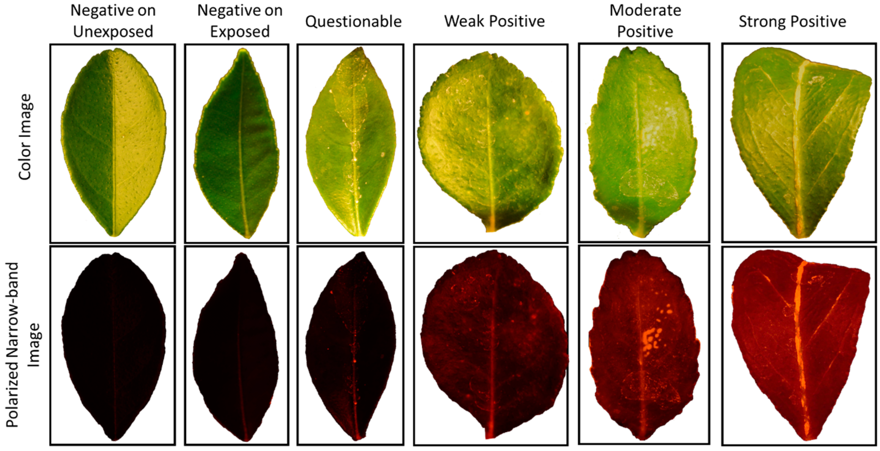
Each region of interest (ROI) in a seedling image was comprised of a single leaf. Since two or three leaves in each seedling image were used for the processing, multiple ROIs, each segmenting a single leaf, were determined manually for each frame. The segmented images were then cropped in size to match the ROI so that each leaf sample was saved as a single image, and background pixels were set to zero. Figure 2 illustrates polarized images of a typical leaf sample from each of the six classes with backgrounds removed along with the corresponding white light color images. The polarized and narrow-band images in Figure 2 had a red tint because seedlings were illuminated with narrow-band light at 595 nm, which is an amber/yellow color light. Since blue and green channels of the camera were not as sensitive at this wavelength, seedling reflectance was solely derived from red channel output. As shown in Figure 2, no visible HLB symptom could be detected in the color images of leaf samples with different HLB statuses. However, there was a notable difference in overall image intensity between HLB-positive and HLB-negative samples in polarized and narrow-band images. As the level of infection increased, the overall intensity increased. This overall increase in gray level intensity was most probably due to the elevated levels of starch shown to correlate with HLB [15].
3.3. Analysis of Variance and Classification Results
Table 3 and Table 4 show several features in each feature set that had p-values less than 0.05 for datasets #1 (early spring) and #2 (late spring), respectively. There were two classes of HLB-negative citrus leaves (samples with zero copy numbers); those from plants that were exposed to feeding by the infected psyllid colony and those from control plants (unexposed). Also, there were four classes of HLB-positive leaves, which were categorized based on their copy number according to the defined copy number ranges in Table 2. A total of 15 pairwise comparisons are presented in three categories; negative samples versus negative samples (comparison 1), negative samples versus positive samples (comparison 2–9), and positive samples versus positive samples (comparison 10–15).
Table 5 and Table 6 show the pairwise classification results for dataset #1 (early spring) and #2 (late spring), respectively. The highlighted grids indicate the maximum average accuracies achieved for each pairwise classification. A summary table is presented showing a comparison between percentages of significant features (ANOVA) and average accuracies (SVM classification) for all 15 comparisons obtained in early spring and those obtained in late spring (Table 7).
4. Discussion
In this study, we have evaluated the capacity of polarizing imaging, optimized for starch detection, to distinguish between healthy and HLB-positive seedlings and between the different levels of infection as determined by QPCR. HLB-positive psyllids were used to inoculate young seedlings in an attempt to achieve uniformity of infection and ensure that early-stage infections were studied. Our overall finding is that polarized imaging, as employed here, can achieve moderate accuracies in identifying HLB-positive seedlings in the first eight months of infection. A total of seven types of feature were analyzed using an ANOVA test and an SVM classifier to obtain percentages of significant features and classification accuracies for each feature set. The STFA feature set had the highest percentages of significant features and the best classification accuracy for dataset #1. In dataset #2, the LSP feature set had the highest percentage of significant features, but the best classification accuracy was achieved using GLCM features. The results of ANOVA tests and SVM classifications using LFDP features were mostly close to average, with a significant improvement in dataset #2.
For 11 comparisons in dataset #1 and 10 comparisons in dataset #2 (Table 3 and Table 4), there was at least one feature that showed significantly different mean values for the corresponding two classes. For comparisons 6, 11, 13, and 15 in dataset #1 and comparisons 1, 2, 3, 7, and 10 in dataset #2, no significant differences in features were obtained. However, features with positive correlations were present in the other comparisons, with several comparisons showing substantially more significant features than the others.
Not surprisingly, among comparisons involving only psyllid-exposed seedlings, the most difficult test was to discriminate between truly negative samples and those that were in the lowest infection status (Questionable), as seen in comparison 6 (Table 5 and Table 6). The highest accuracies among the psyllid-exposed comparisons were between Negative or Questionable for the asymptomatic samples and Strong for the heavily infected set, especially with the earlier imaging data sets (Table 3, comparisons 5 and 12). At the later time of imaging, when further symptom development was a factor, relatively high accuracies were obtained among several comparisons, which included the Moderate class in addition to Strong for the symptomatic, and the Questionable in addition to Negative classes for the asymptomatic samples, as shown in Table 4 (comparisons 8–9 and 11–12). For the early spring dataset (Table 3), the STFA features set had the best overall performance, while, in the late spring set, GLCM features provided the best overall accuracy. LFDP had significantly better performance among the local-based features sets (LBP, LSP, and LFDP). For comparisons 2–5 from the late spring experiment, which included the unexposed samples, the LFDP feature set was clearly more accurate than other features in both datasets.
Several trends are evident in the data summarized in Table 7. For example, in dataset #1, only comparisons between strong positive and negative/questionable classes had the high percentages of significant features (comparisons 5, 9, and 12). However, in dataset #2, comparisons between moderate positive and negative/questionable classes also had high percentages of significant features (comparisons 4, 8, and 11, as well as comparisons 5, 9, and 12). This trend shows that the detection of the level of infection improves as the time passes since the inoculation. Nonetheless, some trends are not related to the HLB status of the seedlings. For example, image analysis was able to distinguish between HLB-negative samples belonging to the unexposed control plants and samples that were exposed to psyllid feeding, with average classification accuracies ranging from 76%–80% (Table 7, comparison 1). Also, modest differences were detected in comparison 2 between the unexposed Negative and exposed Questionable groups. These results suggest that there were variances in image texture resulting from differences in the growing conditions and the level of physiological stress experienced between the control and exposed seedling data sets. This explanation is reasonable since psyllid feeding activity on the test plants was intense during the exposure period, whether or not infection occurred, and absent in the control plants. Wounding that happened during psyllid exposure could easily affect subsequent growth and account for textual differences in the imaging between the control and test data sets. It is clear that the results in comparisons 1 and 2 involving the unexposed seedling data set were unduly influenced by differences regarding growth and stress, not HLB-infection status. More meaningful comparisons are those derived from exposed seedlings only (Table 7, comparisons 6–15). It can be seen that the various classification schemes were able to produce moderate average accuracies (66%–84%) when distinguishing between HLB-negative samples (among exposed plants) and most of the classes of infection ranging from Weak to Strong (Table 5, comparisons 6–9). Similar average accuracies were obtained in comparisons between the different HLB-positive classes (Table 7, comparisons 10–15).
Substantial differences in the average accuracies were also obtained between images taken in early versus late spring. When only plants exposed to psyllid feeding were considered (Table 7, comparisons 6–15), accuracies improved by allowing a greater length of time to pass before imaging; late spring average accuracies were greater (by 3%–7%) than those in early spring. As expected, this finding is consistent with greater accuracy being correlated with an increased development of symptoms. It is interesting to note that in comparisons between unexposed and exposed samples (Table 7, comparisons 1–5), greater average accuracies were obtained in early spring. This result, again, suggests that exposure to psyllid feeding more strongly influenced the imaging when less time had passed between exposure and imaging. Conversely, in comparisons where differences in psyllid exposure were not a factor (Table 7, comparisons 6–15), accuracies improved with the passage of time from exposure as a result of HLB symptom development.
5. Conclusions
In this study, a polarized imaging technique was evaluated for the early detection of HLB disease symptoms in citrus seedlings. Citrus plants were exposed to a CLas-positive population of psyllids for eight weeks. Polarized images were taken of the intact plants at two different times after the period of psyllid feeding. Only 72% of leaf samples obtained from exposed plants had some level of infection; however, there was at least one infected leaf in every exposed plant. Thus, when viewed from a whole seedling basis, it can be concluded that the psyllid feeding infection protocol efficiently transferred CLas to the healthy plants. The polarized imaging technique developed in this study was able to detect the existence of CLas in HLB-affected citrus leaves while they were in presymptomatic and early symptomatic stages, something much more challenging than discriminating between healthy and severely symptomatic leaves. For example, utilizing a variety of classification approaches in the present study, accuracies were achieved that ranged from 68.02% to 94.75% in discriminating seedlings that were exposed but negative from those that were weakly positive for CLas (Table 4). The method developed was also able to determine four levels of infection while leaves were in the nonsymptomatic stage of the disease. Further experiments are required to improve the efficiency of the diagnosis method proposed in this study. For example, it was determined that including lens-to-leaf distance information in a citrus sensing system significantly improved diagnostic accuracy [19]. Although all plants were positioned the same distance from the camera in the present study, different leaves of the same plant were positioned at various distances and planar angles in the images. Therefore, including depth information during image acquisition, something that can be acquired using a depth camera, is one modification that is expected to improve accuracy predictions.
The results of this study suggest that polarized imaging could be incorporated into machine learning approaches for high throughput screening of young citrus plants based on their HLB infection status. A screening protocol of this nature could be used in the assessment of the efficacy of standardized inoculation methods, such as the psyllid feeding approach used here or other methods. Other potential uses for this type of optical sensing approach for HLB detection in citrus include screens for natural resistance, the screening of symptom severity following treatment trials, and for the assessment of improved varieties, GMO-based or otherwise. Although the prediction accuracies demonstrated in the current study were rather modest, these could potentially be improved by combining polarization imaging with fluorescence and reflectivity measurements.
Acknowledgments
We thank William Dawson for the generous use of his psyllid growth room, equipment purchases, and wise council; Reza Ehsani for equipment support; Carol Wetterich for assistance in camera construction and some of the initial imaging using fluorescence; and Cecil Robinson for help and advice regarding the management of the psyllid growth room. We would also like to thank the Citrus Research and Development Foundation for financially supporting this research (CRDF project #880).
Author Contributions
Alireza Pourreza, Won Suk Lee, and William Gurley conceived and designed the experiments. Gurley supervised the inoculation, imaging, and PCR tests, which were conducted by Eva Czarnecka and Lance Verner. Pourreza and Lee developed the image analysis algorithm, conducted the feature extractions and classification, and generated the results.
Conflicts of Interest
The authors declare no conflict of interest. The founding sponsors had no role in the design of the study; in the collection, analyses, or interpretation of data; in the writing of the manuscript; or in the decision to publish the results.
References
- Bravo, C.; Moshou, D.; Orberti, R.; West, J.; McCartney, A.; Bodria, L.; Ramon, H. Foliar disease detection in the field using optical sensor fusion. Agric. Eng. Int. CIGR J. 2004, VI, FP04008. [Google Scholar]
- Karoui, R.; Blecker, C. Fluorescence spectroscopy measurement for quality assessment of food systems—A review. Food Bioprocess Technol. 2011, 4, 364–386. [Google Scholar] [CrossRef]
- Lichtenthaler, H.; Wenzel, O.; Buschmann, C.; Gitelson, A. Plant Stress Detection by Reflectance and Fluorescencea. Ann. N. Y. Acad. Sci. 1998, 851, 271–285. [Google Scholar] [CrossRef]
- Lichtenthaler, H.K.; Schweiger, J. Cell wall bound ferulic acid, the major substance of the blue-green fluorescence emission of plants. J. Plant Physiol. 1998, 152, 272–282. [Google Scholar] [CrossRef]
- Lichtenthaler, H.K. Chlorophylls and carotenoids: Pigments of photosynthetic biomembranes. Methods Enzymol. 1987, 148, 350–382. [Google Scholar]
- Lichtenthaler, H.K.; Buschmann, C. Chlorophylls and carotenoids: Measurement and characterization by UV-VIS spectroscopy. Curr. Protoc. Food Anal. Chem. 2001. [Google Scholar] [CrossRef]
- Mota, A.D.; Rossi, G.; de Castro, G.C.; Ortega, T.A. Portable Fluorescence Spectroscopy Platform for Huanglongbing (HLB) Citrus Disease In Situ Detection. Proc. SPIE 2014, 9003. [Google Scholar] [CrossRef]
- Sankaran, S.; Ehsani, R. Comparison of visible-near infrared and mid-infrared spectroscopy for classification of Huanglongbing and citrus canker infected leaves. Agric. Eng. Int. CIGR J. 2013, 15, 75–79. [Google Scholar]
- Sankaran, S.; Maja, J.M.; Buchanon, S.; Ehsani, R. Huanglongbing (Citrus Greening) Detection Using Visible, Near Infrared and Thermal Imaging Techniques. Sensors 2013, 13, 2117–2130. [Google Scholar] [CrossRef] [PubMed]
- Wetterich, B.C.; Kumar, R.; Sankaran, S.; Junior, J.B.; Ehsani, R.; Marcassa, L.G. A Comparative Study on Application of Computer Vision and Fluorescence Imaging Spectroscopy for Detection of Citrus Huanglongbing Disease in USA and Brazil. J. Spectrosc. 2013, 2013, 841738. [Google Scholar] [CrossRef]
- Wetterich, C.B.; de Oliveira Neves, R.F.; Belasque, J.; Marcassa, L.G. Detection of citrus canker and Huanglongbing using fluorescence imaging spectroscopy and support vector machine technique. Appl. Opt. 2016, 55, 400–407. [Google Scholar] [CrossRef] [PubMed]
- Sankaran, S.; Ehsani, R. Detection of huanglongbing disease in citrus using fluorescence spectroscopy. Trans. ASABE 2012, 55, 313–320. [Google Scholar] [CrossRef]
- Sankaran, S.; Mishra, A.; Maja, J.M.; Ehsani, R. Visible-near infrared spectroscopy for detection of Huanglongbing in citrus orchards. Comput. Electron. Agric. 2011, 77, 127–134. [Google Scholar] [CrossRef]
- Sankaran, S.; Ehsani, R. Visible-near infrared spectroscopy based citrus greening detection: Evaluation of spectral feature extraction techniques. Crop Prot. 2011, 30, 1508–1513. [Google Scholar] [CrossRef]
- Etxeberria, E.; Gonzalez, P.; Achor, D.; Albrigo, G. Anatomical distribution of abnormally high levels of starch in HLB-affected Valencia orange trees. Physiol. Mol. Plant Pathol. 2009, 74, 76–83. [Google Scholar] [CrossRef]
- Gonzalez, P.; Reyes-De-Corcuera, J.; Etxeberria, E. Characterization of leaf starch from HLB-affected and unaffected-girdled citrus trees. Physiol. Mol. Plant Pathol. 2012, 79, 71–78. [Google Scholar] [CrossRef]
- Schneider, H. Anatomy of greening-disease sweet orange shots. Phytopathology 1968, 58, 1155–1160. [Google Scholar]
- Pourreza, A.; Lee, W.S.; Raveh, E.; Ehsani, R.; Etxeberria, E. Citrus Huanglongbing detection using narrow-band imaging and polarized illumination. Trans. ASABE 2014, 57, 259–272. [Google Scholar]
- Pourreza, A.; Lee, W.S.; Ehsani, R.; Schueller, J.K.; Raveh, E. An optimum method for real-time in-field detection of Huanglongbing disease using a vision sensor. Comput. Electron. Agric. 2015, 110, 221–232. [Google Scholar] [CrossRef]
- Pourreza, A.; Lee, W.S.; Raveh, E.; Hong, Y.; Kim, H.-J. Identification of citrus greening disease using a visible band image analysis. In Proceedings of the ASABE Annual International Meeting, Kansas City, MO, USA, 21–24 July 2013. [Google Scholar]
- Pourreza, A.; Lee, W.S.; Etxeberria, E.; Banerjee, A. An evaluation of a vision-based sensor performance in Huanglongbing disease identification. Biosyst. Eng. 2015, 130, 13–22. [Google Scholar] [CrossRef]
- Li, W.; Hartung, J.S.; Levy, L. Quantitative real-time PCR for detection and identification of Candidatus Liberibacter species associated with citrus huanglongbing. J. Microbiol. Methods 2006, 66, 104–115. [Google Scholar] [CrossRef] [PubMed]
- Pourreza, A.; Pourreza, H.; Abbaspour-Fard, M.-H.; Sadrnia, H. Identification of nine Iranian wheat seed varieties by textural analysis with image processing. Comput. Electron. Agric. 2012, 83, 102–108. [Google Scholar] [CrossRef]
- Costa, A.F.; Humpire-Mamani, G.; Traina, A.J.M. An efficient algorithm for fractal analysis of textures. In Proceedings of the 25th SIBGRAPI Conference on Graphics, Patterns and Images (SIBGRAPI), Ouro Preto, Brazil, 22–25 August 2012; pp. 39–46. [Google Scholar]
- Ojala, T.; Pietikäinen, M.; Harwood, D. A comparative study of texture measures with classification based on featured distributions. Pattern Recognit. 1996, 29, 51–59. [Google Scholar] [CrossRef]
- Pourreza, H.R.; Masoudifar, M.; ManafZade, M. LSP: Local similarity pattern, a new approach for rotation invariant noisy texture analysis. In Proceedings of the 18th IEEE International Conference on Image Processing (ICIP), Brussels, Belgium, 11–14 September 2011; pp. 837–840. [Google Scholar]
- Bishop, C.M. Pattern Recognition and Machine Learning, 1st ed.; Springer: New York, NY, USA, 2006. [Google Scholar]
Figure 1.
Local Finite Difference Pattern (LFDP) procedure. (a): a 3 × 3 neighborhood of an image; (b): ranking of the sorted values in the 3 × 3 neighborhood; (c): the sorted values plot as the texture signature of the 3 × 3 neighborhood.
Figure 1.
Local Finite Difference Pattern (LFDP) procedure. (a): a 3 × 3 neighborhood of an image; (b): ranking of the sorted values in the 3 × 3 neighborhood; (c): the sorted values plot as the texture signature of the 3 × 3 neighborhood.
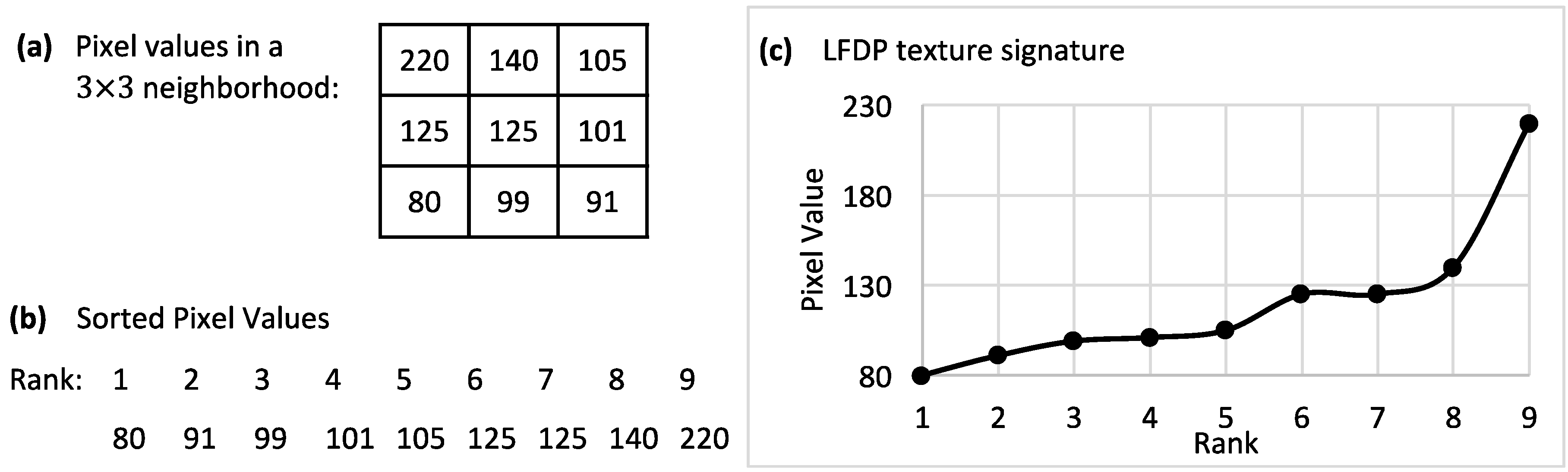
Figure 2.
Color images (top) of leaf samples in six classes with their corresponding polarized and narrow-band images (bottom) acquired by the vision sensor. The overall gray level intensity (shown here as the original red channel) increased in polarized narrow-band images as the level of HLB infection increased.


Table 1.
Finite differences at nine orders ( ) and nine ranks ( ) for the sample 3 × 3 neighborhood in Figure 1.
Table 1.
Finite differences at nine orders ( ) and nine ranks ( ) for the sample 3 × 3 neighborhood in Figure 1.
| 1 | 2 | 3 | 4 | 5 | 6 | 7 | 8 | 9 | ||
|---|---|---|---|---|---|---|---|---|---|---|
| 0th | 80 | 91 | 99 | 101 | 105 | 125 | 125 | 140 | 220 | |
| 1st | 11 | 8 | 2 | 4 | 20 | 0 | 15 | 80 | ||
| 2nd | 3 | 6 | 2 | 16 | 20 | 15 | 65 | |||
| 3rd | 3 | 4 | 14 | 4 | 5 | 50 | ||||
| 4th | 1 | 10 | 10 | 1 | 45 | |||||
| 5th | 9 | 0 | 9 | 44 | ||||||
| 6th | 9 | 9 | 35 | |||||||
| 7th | 0 | 26 | ||||||||
| 8th | 26 | |||||||||
Table 2.
Different classes of Huanglongbing (HLB)-negative and HLB-positive leaf samples corresponding to their infection level and based on their copy number determined from the quantitative polymerase chain reaction (QPCR) test. “Negative on Unexposed” refers to the number of seedlings that were negative in those that were not exposed to the infected psyllids. “Negative on Exposed” refers to the number of seedlings that were exposed to the infected psyllid colony but remained uninfected. The other classes are based on a range of copy numbers of the CLas amplicon present in a 2 μL aliquot of DNA prepared by a uniform isolation protocol.
| Number of Samples | ||||
|---|---|---|---|---|
| Class | Copy Number | Dataset #1 | Dataset #2 | Combined |
| Negative on Unexposed | 0 | 12 | 11 | 23 |
| Negative on Exposed | 0 | 21 | 35 | 56 |
| Questionable | 1–20 | 22 | 17 | 39 |
| Weak Positive | 20–100 | 25 | 14 | 39 |
| Moderate Positive | 100–1000 | 30 | 9 | 39 |
| Strong Positive | >1000 | 17 | 10 | 27 |
| Total | 127 | 96 | 223 | |
Table 3.
ANOVA results for dataset #1 (early spring). Percentage of features in each feature set that had significantly different values (with 5% risk) for a corresponding pair of classes. The last row contains the percentage of significant features in each feature set.
Table 3.
ANOVA results for dataset #1 (early spring). Percentage of features in each feature set that had significantly different values (with 5% risk) for a corresponding pair of classes. The last row contains the percentage of significant features in each feature set.
| Textural Features Set | ||||||||
|---|---|---|---|---|---|---|---|---|
| Pair of Classes | HIST * | GLCM | GLRM | STFA | LBP | LSP | LFDP | Total |
| Number of features | 8 | 10 | 11 | 12 | 6 | 6 | 486 | 539 |
| Neg. vs. Neg. | ||||||||
| 1-Unexposed (−) vs. Exposed (−) | 27.3% | 41.7% | 0.8% | 2.2% | ||||
| Neg. vs. Pos. | ||||||||
| 2-Unexposed (−) vs. Questionable | 18.2% | 16.7% | 0.7% | |||||
| 3-Unexposed (−) vs. Weak (+) | 18.2% | 16.7% | 0.8% | 1.5% | ||||
| 4-Unexposed (−) vs. Moderate (+) | 18.2% | 16.7% | 0.7% | |||||
| 5-Unexposed (−) vs. Strong (+) | 12.5% | 30.0% | 9.1% | 16.7% | 14.2% | 14.1% | ||
| 6-Exposed (−) vs. Questionable | - | |||||||
| 7-Exposed (−) vs. Weak (+) | 12.5% | 33.3% | 0.2% | 1.1% | ||||
| 8-Exposed (−) vs. Moderate (+) | 12.5% | 16.7% | 0.6% | |||||
| 9-Exposed (−) vs. Strong (+) | 25.0% | 40.0% | 18.2% | 41.7% | 66.7% | 22.2% | 23.2% | |
| Pos. vs. Pos. | ||||||||
| 10-Questionable vs. Weak (+) | 1.2% | 1.1% | ||||||
| 11-Questionable vs. Moderate (+) | - | |||||||
| 12-Questionable vs. Strong (+) | 25.0% | 40.0% | 33.3% | 57.0% | 52.9% | |||
| 13-Weak (+) vs. Moderate (+) | - | |||||||
| 14-Weak (+) vs. Strong (+) | 12.5% | 20.0% | 1.0% | 1.5% | ||||
| 15-Moderate (+) vs. Strong (+) | - | |||||||
| Percentage of significant features | 6.7% | 8.7% | 7.3% | 13.3% | 0.0% | 6.7% | 6.5% | 6.6% |
* HIST: Histogram.
Table 4.
ANOVA results for dataset #2 (late spring). Percentage of features in each feature set that had significantly different values (with 5% risk) for a corresponding pair of classes. The last row contains the percentage of significant features in each feature set.
Table 4.
ANOVA results for dataset #2 (late spring). Percentage of features in each feature set that had significantly different values (with 5% risk) for a corresponding pair of classes. The last row contains the percentage of significant features in each feature set.
| Textural Features Set | ||||||||
|---|---|---|---|---|---|---|---|---|
| Pair of Classes | HIST | GLCM | GLRM | STFA | LBP | LSP | LFDP | Total |
| Number of features | 8 | 10 | 11 | 12 | 6 | 6 | 486 | 539 |
| Neg. vs. Neg. | ||||||||
| 1-Unexposed (−) vs. Exposed (−) | - | |||||||
| Neg. vs. Pos. | ||||||||
| 2-Unexposed (−) vs. Questionable | - | |||||||
| 3-Unexposed (−) vs. Weak (+) | - | |||||||
| 4-Unexposed (−) vs. Moderate (+) | 17.1% | 15.4% | ||||||
| 5-Unexposed (−) vs. Strong (+) | 25.0% | 10.0% | 50.0% | 19.1% | 18.4% | |||
| 6-Exposed (−) vs. Questionable | 0.6% | 0.6% | ||||||
| 7-Exposed (−) vs. Weak (+) | - | |||||||
| 8-Exposed (−) vs. Moderate (+) | 10.0% | 9.1% | 66.7% | 52.7% | 48.6% | |||
| 9-Exposed (−) vs. Strong (+) | 25.0% | 10.0% | 27.3% | 16.7% | 100.0% | 35.8% | 34.9% | |
| Pos. vs. Pos. | ||||||||
| 10-Questionable vs. Weak (+) | - | |||||||
| 11-Questionable vs. Moderate (+) | 10.5% | 9.5% | ||||||
| 12-Questionable vs. Strong (+) | 25.0% | 50.0% | 9.9% | 9.8% | ||||
| 13-Weak (+) vs. Moderate (+) | 0.2% | 0.2% | ||||||
| 14-Weak (+) vs. Strong (+) | 25.0% | 16.7% | 0.6% | 1.3% | ||||
| 15-Moderate (+) vs. Strong (+) | 12.5% | 0.2% | ||||||
| Percentage of significant features | 7.5% | 2.0% | 2.4% | 2.2% | 4.4% | 13.3% | 9.8% | 9.3% |
Table 5.
Pairwise classification results achieved for dataset #1 (early spring). The highest value in a series is highlighted. Values in each row show different classification accuracies achieved for a pair of classes that is illustrated in the first column. Values in each column show the classification accuracies achieved for all pair of classes using the types of textural features that are illustrated in the second row.
| Textural Features Set | ||||||||
|---|---|---|---|---|---|---|---|---|
| Pair of Classes | HIST | GLCM | GLRM | STFA | LBP | LSP | LFDP | Average |
| Neg. vs. Neg. | ||||||||
| 1-Unexposed (−) vs. Exposed (−) | 72.2% | 79.6% | 84.7% | 85.1% | 78.7% | 80.9% | 79.9% | 80.2% |
| Neg. vs. Pos. | ||||||||
| 2-Unexposed (−) vs. Questionable | 72.3% | 76.0% | 82.3% | 81.7% | 84.4% | 72.9% | 76.6% | 78.0% |
| 3-Unexposed (−) vs. Weak (+) | 80.2% | 82.9% | 83.4% | 85.4% | 84.7% | 78.6% | 94.0% | 84.2% |
| 4-Unexposed (−) vs. Moderate (+) | 70.8% | 79.0% | 85.2% | 83.4% | 83.7% | 79.9% | 82.2% | 80.6% |
| 5-Unexposed (−) vs. Strong (+) | 81.1% | 82.0% | 84.8% | 85.3% | 80.7% | 84.0% | 84.5% | 83.2% |
| 6-Exposed (−) vs. Questionable | 64.0% | 60.2% | 64.9% | 74.5% | 65.6% | 63.4% | 68.6% | 65.9% |
| 7-Exposed (−) vs. Weak (+) | 74.9% | 74.5% | 71.9% | 83.7% | 73.4% | 69.0% | 76.9% | 74.9% |
| 8-Exposed (−) vs. Moderate (+) | 67.0% | 75.1% | 75.2% | 76.0% | 64.2% | 69.9% | 66.4% | 70.5% |
| 9-Exposed (−) vs. Strong (+) | 77.2% | 74.7% | 81.0% | 84.0% | 69.8% | 74.3% | 71.7% | 76.1% |
| Pos. vs. Pos. | ||||||||
| 10-Questionable vs. Weak (+) | 74.2% | 74.7% | 68.3% | 73.2% | 68.2% | 71.5% | 74.4% | 72.1% |
| 11-Questionable vs. Moderate (+) | 71.8% | 66.8% | 69.9% | 61.9% | 65.8% | 69.9% | 71.2% | 68.2% |
| 12-Questionable vs. Strong (+) | 75.8% | 75.7% | 80.1% | 71.9% | 76.4% | 80.3% | 80.4% | 77.2% |
| 13-Weak (+) vs. Moderate (+) | 64.8% | 66.0% | 61.0% | 58.9% | 63.9% | 64.2% | 57.6% | 62.3% |
| 14-Weak (+) vs. Strong (+) | 72.1% | 71.1% | 70.6% | 76.3% | 66.8% | 67.1% | 72.8% | 71.0% |
| 15-Moderate (+) vs. Strong (+) | 72.8% | 73.5% | 71.6% | 73.5% | 73.7% | 73.9% | 73.0% | 73.2% |
| Average | 72.7% | 74.1% | 75.7% | 77.0% | 73.3% | 73.3% | 75.4% | 74.5% |
Table 6.
Pairwise classification results achieved for dataset #2 (late spring). The highest value in a series is highlighted. Values in each row show different classification accuracies achieved for a pair of classes that is illustrated in the first column. Values in each column show the classification accuracies achieved for all pairs of classes using the types of textural features that are illustrated in the second row.
| Textural Features Set | ||||||||
|---|---|---|---|---|---|---|---|---|
| Pair of Classes | HIST | GLCM | GLRM | STFA | LBP | LSP | LFDP | Average |
| Neg. vs. Neg. | ||||||||
| 1-Unexposed (−) vs. Exposed (−) | 79.2% | 79.5% | 77.9% | 69.4% | 77.1% | 74.6% | 77.3% | 76.4% |
| Neg. vs. Pos. | ||||||||
| 2-Unexposed (−) vs. Questionable | 75.0% | 67.9% | 65.8% | 74.7% | 68.8% | 61.0% | 80.3% | 70.5% |
| 3-Unexposed (−) vs. Weak (+) | 72.0% | 65.5% | 79.5% | 78.4% | 64.1% | 69.4% | 81.7% | 73.0% |
| 4-Unexposed (−-) vs. Moderate (+) | 90.7% | 77.3% | 76.8% | 72.6% | 65.6% | 83.9% | 80.6% | 78.2% |
| 5-Unexposed (−) vs. Strong (+) | 77.9% | 83.4% | 74.9% | 72.6% | 76.3% | 88.7% | 81.8% | 79.4% |
| 6-Exposed (−) vs. Questionable | 66.9% | 75.9% | 68.4% | 73.1% | 74.6% | 66.1% | 79.9% | 72.1% |
| 7-Exposed (−) vs. Weak (+) | 69.8% | 77.1% | 87.9% | 94.8% | 68.0% | 72.2% | 76.3% | 78.0% |
| 8-Exposed (−) vs. Moderate (+) | 77.7% | 95.0% | 90.9% | 79.6% | 77.0% | 80.7% | 85.6% | 83.8% |
| 9-Exposed (−) vs. Strong (+) | 86.0% | 86.4% | 85.9% | 83.8% | 76.8% | 80.1% | 86.2% | 83.6% |
| Pos. vs. Pos. | ||||||||
| 10-Questionable vs. Weak (+) | 66.9% | 72.3% | 78.1% | 98.1% | 71.6% | 60.0% | 67.9% | 73.5% |
| 11-Questionable vs. Moderate (+) | 90.1% | 91.0% | 91.4% | 76.8% | 84.4% | 75.5% | 79.2% | 84.0% |
| 12-Questionable vs. Strong (+) | 85.6% | 86.8% | 81.9% | 78.2% | 80.4% | 78.0% | 85.0% | 82.3% |
| 13-Weak (+) vs. Moderate (+) | 89.0% | 79.8% | 85.5% | 77.5% | 65.7% | 78.3% | 70.6% | 78.1% |
| 14-Weak (+) vs. Strong (+) | 81.9% | 81.2% | 68.6% | 78.0% | 66.4% | 82.4% | 78.8% | 76.8% |
| 15-Moderate (+) vs. Strong (+) | 92.0% | 88.8% | 76.5% | 72.1% | 59.8% | 63.4% | 62.4% | 73.6% |
| Average | 80.0% | 80.5% | 79.3% | 78.6% | 71.8% | 74.3% | 78.2% | 77.5% |
Table 7.
Comparison of percentages of significant features from the ANOVA test and average accuracies for SVM classifications between early and late spring. Comparisons with the unexposed data set (negative control) have been removed in the two rightmost columns (comparisons 6–9 and 10–15). Student’s t-test indicated >95% significance between early and late spring averages for comparisons 1–5 and 10–15 and >91% for comparisons 6–9.
| ANOVA | SVM Classification | |||
|---|---|---|---|---|
| Pair of Classes | Early Spring | Late Spring | EARLY SPRING | Late Spring |
| Neg. vs. Neg. | ||||
| 1-Unexposed (−) vs. Exposed (−) | 2.2% | - | 80.2% | 76.4% |
| Neg. vs. Pos. | ||||
| 2-Unexposed (−) vs. Questionable | 0.7% | - | 78.0% | 70.5% |
| 3-Unexposed (−) vs. Weak (+) | 1.5% | - | 84.2% | 73.0% |
| 4-Unexposed (−) vs. Moderate (+) | 0.7% | 15.4% | 80.6% | 78.2% |
| 5-Unexposed (−) vs. Strong (+) | 14.1% | 18.4% | 83.2% | 79.4% |
| Average (comparisons 1–5) | 4.3% | 8.4% | 81.5% | 75.2% |
| 6-Exposed (−) vs. Questionable | - | 0.6% | 65.9% | 72.1% |
| 7-Exposed (−) vs. Weak (+) | 1.1% | - | 74.9% | 78.0% |
| 8-Exposed (−) vs. Moderate (+) | 0.6% | 48.6% | 70.5% | 83.8% |
| 9-Exposed (−) vs. Strong (+) | 23.2% | 34.9% | 76.1% | 83.6% |
| Average (comparisons 6–9) | 8.3% | 27.8% | 71.9% | 79.4% |
| Pos. vs. Pos. | ||||
| 10-Questionable vs. Weak (+) | 1.1% | - | 72.1% | 73.5% |
| 11-Questionable vs. Moderate (+) | 0.0% | 9.5% | 68.2% | 84.0% |
| 12-Questionable vs. Strong (+) | 52.9% | 9.8% | 77.2% | 82.3% |
| 13-Weak (+) vs. Moderate (+) | - | 0.2% | 62.3% | 78.1% |
| 14-Weak (+) vs. Strong (+) | 1.5% | 1.3% | 71.0% | 76.8% |
| 15-Moderate (+) vs. strong (+) | 0.0% | 0.2% | 73.2% | 73.6% |
| Average (comparisons 10–15) | 9.3% | 3.5% | 70.7% | 78.0% |
© 2017 by the authors. Licensee MDPI, Basel, Switzerland. This article is an open access article distributed under the terms and conditions of the Creative Commons Attribution (CC BY) license (http://creativecommons.org/licenses/by/4.0/).
Share and Cite
MDPI and ACS Style
Pourreza, A.; Lee, W.S.; Czarnecka, E.; Verner, L.; Gurley, W. Feasibility of Using the Optical Sensing Techniques for Early Detection of Huanglongbing in Citrus Seedlings. Robotics 2017, 6, 11. https://doi.org/10.3390/robotics6020011
AMA Style
Pourreza A, Lee WS, Czarnecka E, Verner L, Gurley W. Feasibility of Using the Optical Sensing Techniques for Early Detection of Huanglongbing in Citrus Seedlings. Robotics. 2017; 6(2):11. https://doi.org/10.3390/robotics6020011
Chicago/Turabian StylePourreza, Alireza, Won Suk Lee, Eva Czarnecka, Lance Verner, and William Gurley. 2017. "Feasibility of Using the Optical Sensing Techniques for Early Detection of Huanglongbing in Citrus Seedlings" Robotics 6, no. 2: 11. https://doi.org/10.3390/robotics6020011
Note that from the first issue of 2016, this journal uses article numbers instead of page numbers. See further details here.