
A New Combined Vision Technique for Micro Aerial Vehicle Pose Estimation
by
 ,
,
Haiwen Yuan
1,2,* ,
,
Changshi Xiao
1,3,4,*,
Supu Xiu
1,
Yuanqiao Wen
1,3,4,
Chunhui Zhou
1,3 and
Qiliang Li
2,* 1
School of Navigation, Wuhan University of Technology, Wuhan 430063, China
2
Electrical & Computer Engineering, George Mason University, Fairfax, VA 22030, USA
3
Hubei Key Laboratory of Inland Shipping Technology, Wuhan 430063, China
4
National Engineering Research Center for Water Transport Safety, Wuhan University of Technology, Wuhan 430063, China
*
Authors to whom correspondence should be addressed.
Robotics 2017, 6(2), 6; https://doi.org/10.3390/robotics6020006
Submission received: 5 December 2016
/
Revised: 20 February 2017
/
Accepted: 23 March 2017
/
Published: 28 March 2017
(This article belongs to the Special Issue Robotics and 3D Vision)
Abstract
:In this work, a new combined vision technique (CVT) is proposed, comprehensively developed, and experimentally tested for stable, precise unmanned micro aerial vehicle (MAV) pose estimation. The CVT combines two measurement methods (multi- and mono-view) based on different constraint conditions. These constraints are considered simultaneously by the particle filter framework to improve the accuracy of visual positioning. The framework, which is driven by an onboard inertial module, takes the positioning results from the visual system as measurements and updates the vehicle state. Moreover, experimental testing and data analysis have been carried out to verify the proposed algorithm, including multi-camera configuration, design and assembly of MAV systems, and the marker detection and matching between different views. Our results indicated that the combined vision technique is very attractive for high-performance MAV pose estimation.
1. Introduction
In recent years, micro aerial vehicles have shown amazing capability in performing certain difficult tasks and movements, such as exact landing [1], team cooperation [2], building blocks [3], etc. In performing these tasks, state estimation for the aerial vehicles must be precisely obtained and be carried out in a real-time format because any small error or delay may lead to a complete failure. Therefore, the perception of environment and pose of MAVs is important for precise and real-time control. However, in a conventional GPS (Global Position System)-Inertial system, GPS is not reliable enough to deal with the task due to signal blockage or multi-path scattering. The inertial measurement unit (IMU) is able to offer nice pose measurements but suffers from accumulative error over time. Therefore, it needs frequent correction [4]. Although Light Detection and Ranging (LIDAR) can be used to explore the surrounding environment and calculate the relative pose of a MAV, its size and weight are out of the range of the load capacity of a micro aerial robot.
In comparison, the most-adopted method follows a vision-based approach, which is able to provide enough accuracy to satisfy the needs for these MAV tasks, such as take-off, landing, indoor navigation, etc. State estimation for the MAV can be defined as the process of tracking the three-dimensional (3D) pose of the vehicle. The vision-based approach has been intensively studied and recently developed into many different methods categorized by different state estimation methods. According to the arrangement of cameras, the vision-based state estimation can be roughly divided into two categories: onboard navigation and on-ground navigation. Onboard navigation refers to a MAV that tracks some structured or natural object to achieve self-state by using onboard vision, such as relative target and landmark navigation [5,6,7], visual odometry (VO) [8,9], simultaneous localization and mapping (SLAM) [10,11], etc. In the early stage of onboard navigation, relative target and landmark navigation were used to estimate the relative MAV pose via onboard vision [5,6,7], where the structure of the reference targets/landmarks is known. Then methods based on structure from motion (SFM), SLAM, and VO have been proposed one by one. Using the methods, the MAV pose can be estimated by tracking some typical features from the natural scene. Without the transformation from image plane to 3D space, bio-inspired optical flow techniques have been also applied to directly infer the MAV pose and motion depending on only the information in images [12,13]. Alternatively, a MAV calculates its pose by an external visual measuring system, which is usually called on-ground navigation. In such a system, one or more cameras are distributed in the surrounding and have the ability to capture the image data about MAVs in real time. Normally as a testbed, on-ground navigation is applied to test the algorithms of robot global positioning, control, and planning. In this situation, either carrying load or computation capacity is no longer considered to be a problem. Even though current studies mainly focus on onboard vision, like the above-mentioned methods, on-ground navigation is worth studying as well [14,15,16,17,18]. However, these systems used only the triangulation method in stereo camera configuration or the PNP (perspective-n-point) method in single camera configuration.
For the on-ground navigation method, we have developed a new combined vision technique to significantly enhance the real-time MAV pose estimation, and built an on-ground visual system to test it. In this CVT, two positioning strategies with different constraints have been integrated by a particle filter framework at the same time: multi-view triangulation and monocular perspective-3-point (P3P) algorithms. The multi-view triangulation algorithm is based on the intersection of different views, while the monocular P3P technique is based on the shape change of a rigid body in the image. The visual system is expected to have a more stable performance when these two location methods (mono-view P3P and multi-view triangulation) are considered simultaneously by a PF framework.
The remainder of this paper is organized as follows: Section 2 reviews the related work of visual measurement in MAV navigation. A summary of the visual system including hardware and software is presented in Section 3. In the hardware part, the MAV and camera configurations are introduced. In the software part, the feature point detection and multi-camera calibration are also described. Section 4 illustrates the proposed CVT visual algorithm which is used to calculate MAV poses by integrating the two different methods. Finally, experiment testing results are demonstrated and conclusions will be drawn in Section 5 and Section 6, respectively.
2. Previous Research in On-Ground Visual Navigation for MAV Pose Estimation
MAV pose estimation in different applications and many advanced strategies to achieve this task have been intensively studied for the past two decades. On-ground visual navigation is a commonly used strategy for motion capture, which employs a set of external cameras with known camera parameters to track and locate MAV. These cameras are usually installed around to observe the flight in space simultaneously. This strategy is usually applicable to a limited space but with good accuracy.
For example, the VICON system (Vicon Motion Systems Ltd., Oxford, UK), a commercial product, is able to track and locate more than one robot at the same time. The system exhibits a good performance of positioning accuracy and processing rate. Based on this system, MAV control and navigation have been well demonstrated in [19,20,21], where MAVs are controlled by the feedback of the visual system to dance, play musical instruments, build houses, etc. However, such a configuration requires multiple high-speed external IR cameras and is too expensive. An indoor test-bed named RAVEN (Real-time indoor Autonomous Vehicle test ENvironment), based on VICON system, has been developed by the Aerospace Control Lab [22] for autonomous navigation of multiple rotorcrafts, where vision is the only manner used for MAV pose estimation. The test-bed acquired pose information by detecting and locating markers installed around MAV. The markers are usually beacons or reflection spheres which are easy to recognize by infrared camera. Therefore, such a system has a high resolution for location positioning and has been used to perform complicated tasks, such as autonomous landing, charging, fancy flying, and multi-MAV motion planning.
Martínez et al. [14] proposed two visual manners including onboard vision and on-ground vision to enable MAV automation. One detects and tracks the planar structure by an onboard camera. The other one is a 3D reconstruction of the position of MAV by an on-ground camera system. The on-ground camera system consists of three visible light cameras, by which the color markers attached to the flying vehicle can be tracked and located. However, the results are rough because the markers on the aircrafts are too large and the view is limited. In the work by Faessler et al. [15], the MAV pose estimation was done with the P3P algorithm. An infrared camera is used as the major sensor in such a system to assist detection. However, it takes a certain calculation time to distinguish markers attached to different positions of the aerial body, as they look the same in the infrared image. Different from the above, Hyondong et al. [16] employed a visible light camera instead of an infrared camera to detect and track indoor MAV pose with color balls as the markers. Since onboard markers are attached to the pre-defined location and have different color features, the position and attitude of MAV could be recognized by color feature and triangulation. In addition, an extended Kalman filter (EKF) framework integrated with MAV dynamic was introduced to improve the performance of the visual measurement system. For example in [17], two stationary and upward-looking cameras were placed on the ground to track four black balls attached to the helicopter. The errors between the positions of the tracked balls and pre-specified references are taken as the visual feedback control input. A pair of ground and onboard cameras was employed for the problem of quadrotor pose estimation [18]. The two cameras were set to face each other to estimate the full 6-degrees-of-freedom (DOF) pose of MAVs.
Different from the above-mentioned works, this paper did not pay too much attention to the system configuration, but focused on how to make use of the image data from a visual system to archive a stable pose estimation. In this work we will try to consider the two kinds of location methods (mono-view P3P and multi-view triangulation) simultaneously by a PF framework.
3. Description of the Visual Measurement System
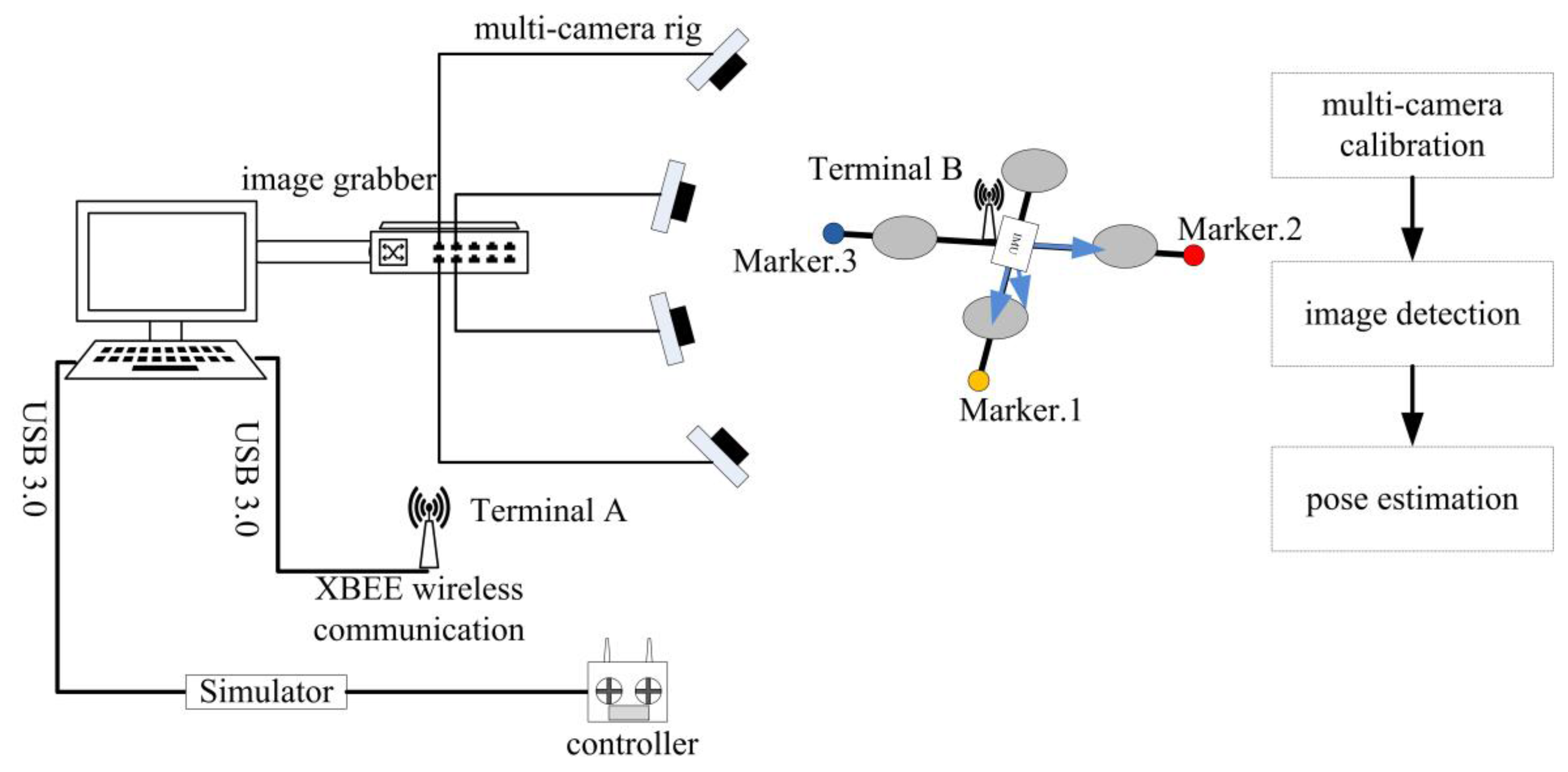
The on-ground visual measurement system is designed to test the proposed CVT and includes the cameras, image grabber, PC processor, and self-built MAV with markers. The major focuses in this study are calibration of the multi-camera system, MAV system design, and MAV detection.
3.1. Multi-Camera System Calibration
Before starting the measuring work, the multi-camera system should be calibrated to acquire a mapping between the features in the real 3D space and the 2D image. By considering the basic pinhole camera model, the calibration setups are separated into two setups. The first setup is for intrinsic parameter calibration where each camera is individually calibrated with the Bouguet camera calibration toolbox [23]. The second setup is for extrinsic parameter calibration carried out by the multi-camera self-calibration toolbox [24].
In our measurement system (see Figure 1), four analog CCD (Charge Coupled Device) cameras are connected to a PC station via a general 8-channel image grabber. So the data source from the cameras can be captured synchronously and processed in real-time with the help of the OpenCV library. At first, we use several image chessboards from different camera views and calibrate the four intrinsic parameters of every camera, including the focal length (fx, fy) and principal point (μ0, ν0). These parameters constitute the internal matrix (K-matrix) in the imaging model, which can be written as:
where is the 2D image point represented by a homogeneous vector , is the 3D world point represented by a homogeneous four-vector , and s is a scalar representing the depth information. R is the rotation transform matrix and t is the translation transform matrix from the world frame to camera frame. R, t, and K-matrix constitute the mapping between the 3D world and 2D image, which can be called the Projective matrix (P-matrix).
Once K-matrix is acquired, only seven parameters remain unknown for every camera, including the scalar s, 3-vector r, and 3-vector t, respectively, in the P-matrix. All the image points, 3D-world points, and camera projectives from all the cameras can be put into the following equation:
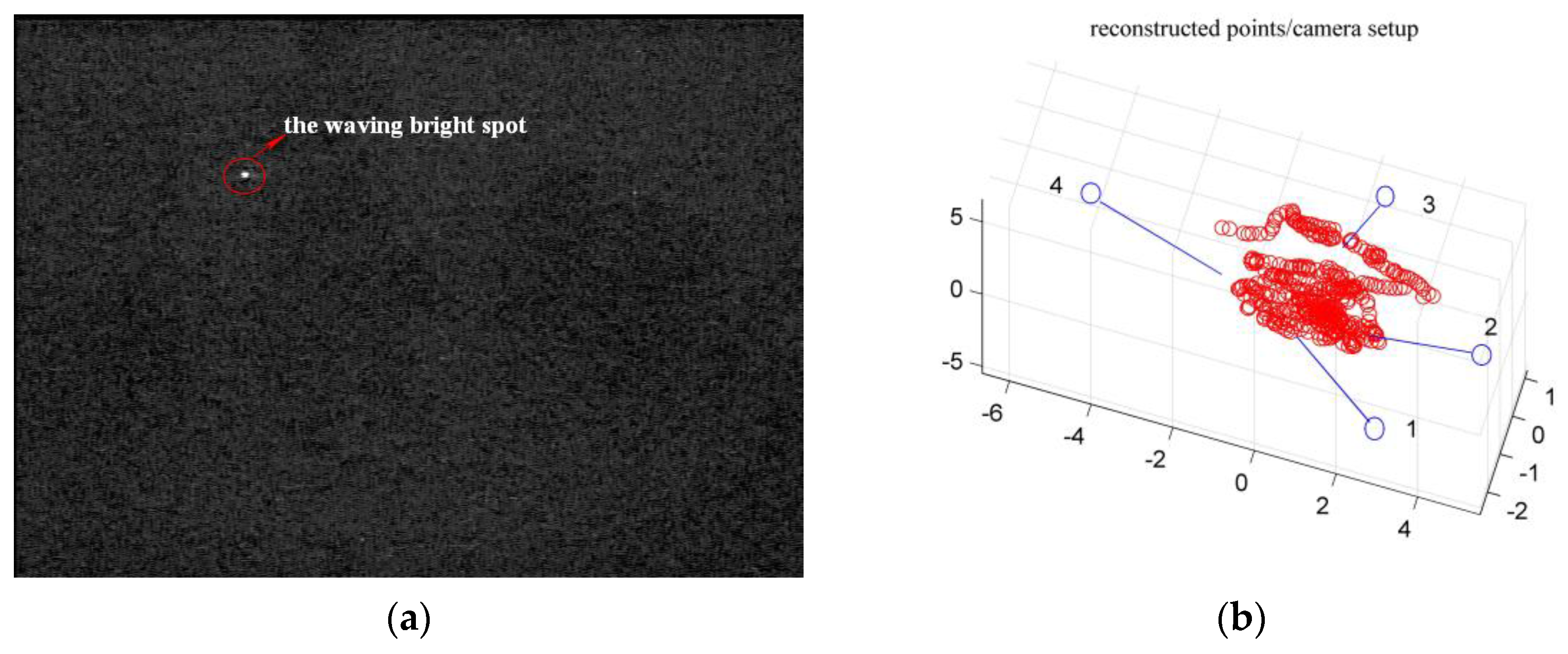
Based on the equation above, Ws can be factorized to recover the projective motion P and the projective shape X if enough noiseless points can be collected. During the calibration of extrinsic parameters, the bright spots will be waved through the working volume of the camera system, as shown in Figure 2a. Besides intrinsic parameters, the coordinates of the bright spots in all images are the known information. The detailed computation and calibration processes have been previously explained [24]. With the multi-camera self-calibration toolbox, not only the extrinsic parameters of all cameras but also the coordinates of bright spots in the 3D space can be recovered. This is shown in Figure 2b.
3.2. MAV Design and Detection
As shown in Figure 3, the MAV system is built with only one airframe, four speed controllers and rotors and propellers, onboard microcontroller, communication module, and IMU sensor. In the system, the main part for control and information processing is operated by a computer (PC) on the ground. The onboard microcontroller, STM32F103 (STMicroelectronics, Shanghai, China), is in charge of receiving speed command from the ground PC to generate corresponding Pulse-Width Modulation (PWM) for the speed controllers to control the four motors. Also, the microcontroller can be utilized to capture the inertial information from the IMU sensor and send it to the ground PC in real time. The IMU, MPU9150 (InvenSense, San Jose, CA, US), is a unique sensor on the drone, which is continuously sending measurements of the attitude angle, acceleration, and angular velocity to the microcontroller at 100 Hz. The module Xbee PRO 900HP S3B is responsible for the communication between the onboard and ground PC, which is able to work in full-duplex mode. A joystick is connected to the ground PC by a simulator and is used to change the flight state of the MAVs. In order to conveniently and efficiently test the control system in the lab, the quadrotor is mounted on a plank via a cardan joint so that its state can be flexibly adjusted without flying far away.
As color is one of the most distinct features in the environment, we set three different color balls around the airframe as markers for detection. Firstly, Gaussian filtering is done with a five-by-five patch for every image to remove some sharp and unnecessary information. Because of different colors, the three balls could be well segmented from the scene in HSV (hue, saturation, value) space. However, the measurements in the images from different views (cameras) are not independent with each other in the multi-camera configuration. It should be noted that there is an epipolar geometry constraint between every two fixed views. The constraint allows the correspondence of image point x from one view and image point x’ from the other view, which can be written as:
where F is the fundamental matrix that contains the information of the two cameras’ intrinsic and extrinsic parameters and can be acquired in advance according to Equation (4),
where K′ and K are the intrinsic matrices of the two cameras, while R and t represent the 3 × 3 rotation matrix and the 3 × 1 translation matrix. From this equation, we can determine the corresponding x′ in the other view along the epipolar line once the point x in one view is found. As a result, the detection in all views takes less processing time and improves noise immunity. The results of the marker detection are shown in Figure 4a–e, showing that the detection is steady and the mean error is less than one pixel.
4. Pose Estimation
4.1. Marker Location and MAV Pose Computation
It is noted that there is a unique solution to determine the position of a 3D point in the two-view geometry by triangulation. Given the parameters of one camera, every point in the image can be used by the two equations to determine the three unknown coordinates of the corresponding point in 3D space according to the projection model (Equation (2)). Therefore, in the case of two or more than two views, there are more than enough equations to obtain the solution. The more equations that are considered, the higher accuracy the solution has. The fundamentals of the triangulation method are shown in Figure 5a. In this method, the color marker represented by point X can be located in the 3D world based on the knowledge of the corresponding positions in the image planes taken by Camera 1–Camera N. The detailed computation is shown in Equation (5), which is a combination of all the projective equations,
where denotes the homogeneous coordinate of the marker in image plane i, denotes the projective matrix of camera i, and denotes the homogeneous coordinate of the marker in the 3D world.
At the same time, by using the known relative relations among the three color markers on the rigid body, the marker position and the rigid body pose relative to the camera frame can be derived. This method is a so-called P3P problem, where the only given information is the actual distances between each two markers. The details of the P3P method are shown in Figure 5b. The image point with focal normalization is calculated with Equation (6). The side lengths of the triangle structured from the markers M1, M2, and M3 are denoted by a, b, and c, respectively. In fact, the vector has the same direction with the unit vector , which is expressed in Equation (7).
Consequently, the cosine of the angles between the three unit vectors could be determined by Equation (8). Therefore, the three equations about the distance d1, d2, and d3 between the points M1–M3 and the center of camera can be obtained according to the cosine law, as described in Equation (8). The equations can be solved by linear iteration with two real solutions of d1–d3.
Finally, the positions of the three markers M1–M3 relative to the camera reference frame can be determined by Equation (10). Since the camera orientation in the 3D world frame has been calibrated in advance, the positions of the three markers M1–M3 relative to the 3D world frame can be also calculated.
Because the positions of markers M1–M3 on the MAV are given, the pose of the MAV relative to the 3D world reference can be determined from the discussion above. The MAV pose contains both position and attitude, as shown in Figure 5c. The center of the markers M1 and M2 is defined as the MAV position. In the rotation matrix , the three vectors, , , and represent the , , direction of the body frame in the 3D world coordinates, respectively. As shown in Equation (11), the MAV body reference frame can be built with the vector from the center between M2 and M3 to M1 as , and the vector from M2 to M3 as , and to be determined by the right-hand rule,
where can be determined by the cross product of and following the orthogonality of R. Now, the rotation and translation relationship between the body frame and the world frame has been derived. The three attitude angles (roll, pitch, yaw) of the MAV can be solved by the Rodriguez transformation expressed in Equation (12):
where , and represent yaw, pitch, and roll angle, respectively. It should be noted that each angle needs to be adjusted to a different range so that it can be consistent with the IMU output. In general, for a rigid body (MAV) the three attitude angles (roll, pitch, and yaw) should have a defined range and change direction. For example, the range of the roll angle is set to [−180°, 180°], the range of the pitch angle is set to [−90°, 90°], and the range of the yaw angle is set to [0°, 360°]. However, the computation result acquired directly from the visual system is [0°, 360°]. So it is necessary that the two sets of attitudes are adjusted to be consistent. The adjustment is also called “normalization”.
4.2. Pose Estimation
As the measurement is taken from the visual system, the MAV pose is continuously calculated from multi-view triangulation and mono-view P3P, which will be used to correct or update the state of MAVs in a fusion framework. In general, inertial measurements taken at high rate (100 Hz–2 kHz) are fused with lower rate exteroceptive updates from vision, or GPS. For the MAV pose estimation, conventional approaches are based on the indirect formulations of Extended or Unscented Kalman Filters and Particle Filters (PF). For a multiple-camera measurement of one quantity at an approximate same time, the framework in this work is based on the indirect formulation of an iterated PF, where the state prediction is driven by IMU.
With as a right-hand inertial frame, defines a body-fixed frame with its center at the center of mass of the vehicle. The ground 3D-world reference in the visual system is set to be consistent with the inertial frame. The motion model of the rigid body can be derived based on the kinematic equation of attitude and Newton’s equation of motion, as expressed in Equation (13). is the position of the center of mass of the vehicle in frame I. is the linear velocity in frame I. is the angular velocity of the airframe with respect to the frame B. The attitude of the rigid body is given by the rotation matrix .
The operator maps into an anti-symmetric matrix. m represents the rigid object’s mass. represents the inertia matrix which is a constant. The vectors F and represent the principal non-conservative forces and moments applied to the rotorcraft airframe by the aerodynamics of the rotors, respectively. It is difficult for a PF to deal with high dimensional states. This is because the filter is likely to be divergent as the dimensions increase. The estimated state of a MAV consists of the linear velocity , the attitude angle in the inertial frame, the acceleration, and the angular velocity in the body frame. The acceleration and the angular velocity measured by the IMU are supposed to be the sum of the real value, a bias noise, and a Gaussian noise. Therefore, the number of the PF state is 12, as expressed in the following,
Measurements of the MAV state include its position and attitude in the inertial reference coordinate system. Measurement noises are complicated and mainly come from camera calibration, marker detection, and varying environmental conditions. A particle filter is applied to deal with the noises, because it is capable of modeling and canceling the random noise. Such a particle filter is able to simulate the true state of the MAV and many measurements for one state by using different testing methods with the large number of particles in the filter. Therefore, it is used to estimate the state of the MAV in this work.
Similar to other filter frameworks [25,26,27], our estimation based on PF mainly consists of the predicting and the updating periods. The detailed process is shown in Figure 6. During the predicting period, the state of every particle evolves from xk to xk + 1 driven by the IMU based on the motion model discussed above, with fixed weights for the moment. This is followed by the updating period, when the weights of all particles are adjusted more than once. The weights are proportional to the separation of the predicted state and the measurement in every updating step. At first, the weights of all particles are adjusted one by one based on the measurement results from each camera. Then, after the updating period, the particle weights based on multi- and mono-view measurements are normalized. As a result, the state of each particle is estimated by accumulating the product of the particle and its weight. In addition, the particles with little weight will be abandoned, while particles with large weight will be resampled. As a result, the particles to be measured are always enough in the procedure.
5. Experiments and Analyses
The vision-based pose estimation algorithm is tested in our laboratory with a small quadrotor system shown in Figure 7. A visual system is set up with four cameras and a PC with an image grabber. As shown in Figure 7, the quadrotor is flying in the view of the visual system. Its position and attitude relative to the ground 3D reference frame can be calculated by the above-mentioned procedure. The low-cost visible light cameras employed in the system are distributed around a 4 m × 3 m × 3 m testing room.
5.1. Pose Computation Results
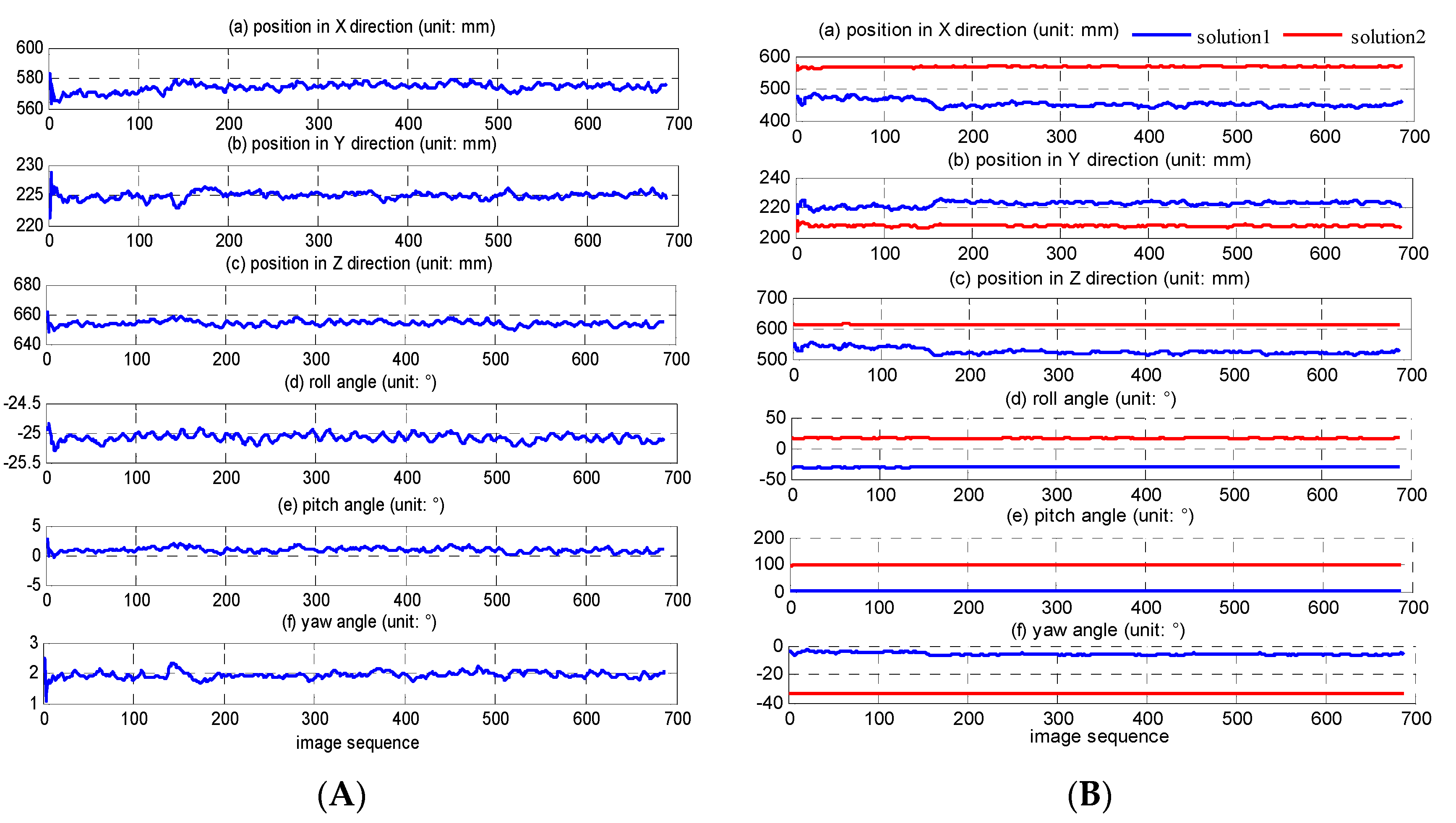
When the positions of the three markers in the image are available, the location of the MAV can be calculated by multi- or mono-view geometry. As shown in Figure 8A,B, the position and attitudes of the testing MAV are calculated by using the two methods, respectively. On account of the P3P method introduced in Section 4, two set of solutions are obtained and are discriminative with red and blue lines in Figure 8B. Even though the two solutions of the position calculation are almost similar, the small disparity would give rise to a large difference on the following attitude angle calculations. It could be observed that one of the two solutions is more close to the solution of the triangulation displayed in Figure 8A. The other solution could be discarded using the triangulation solution as the reference. As a result, this provides a solving method to distinguish the two solutions from P3P. Then by calculating the position and the attitudes continuously, the corresponding histograms about the multi-and mono-view measurements are shown in Figure 9 and Figure 10, respectively. This information could help us understand in advance some performance of the two location methods, such as stability, if the results of the methods are regarded as measurements of the filter framework. Through the histograms, each measured variable, whether it is position or attitude, is centered on a fixed value and changes around it.
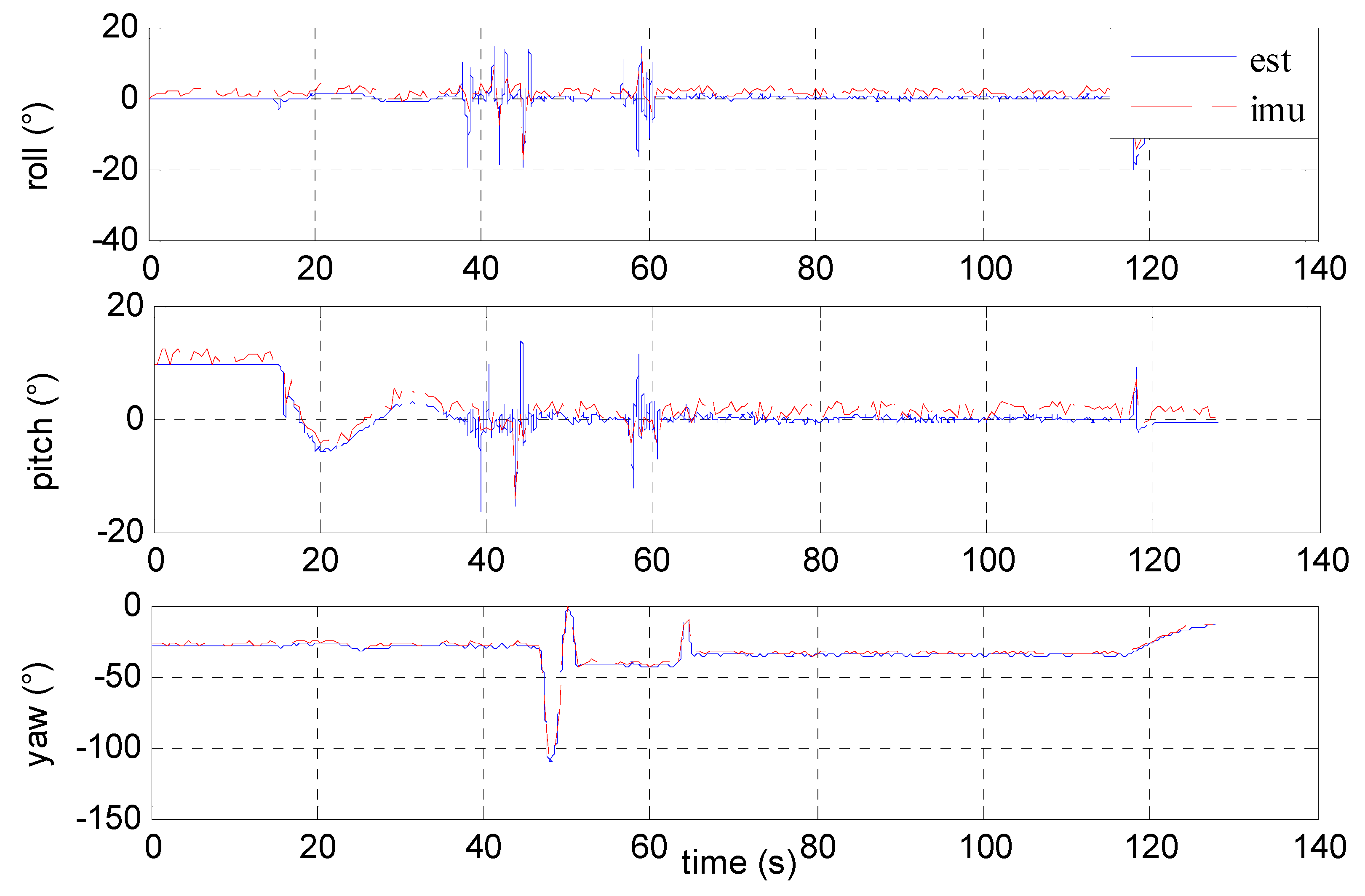
In Figure 11, we compared the estimated attitude angles with the attitude and heading reference system (AHRS) to verify the validity of the visual system. The precision of AHRS is 0.5°–1° and the resolution is 0.1°. As shown in Figure 11, both the IMU and visual measurements are obtained and displayed at the same time when the quadrotor is fixed on the plank via cardan lock. The results indicated that the visual measurements including roll, pitch, and yaw angles are quite consistent with the IMU data. This comparison indicated that the proposed technique is quite accurate.
5.2. MAV Pose Estimation
It is necessary to model and study the noise in the two measurements from the visual system in order to finally achieve an accurate design parameter of the filter. The noise model from the measurements has been obtained by analyzing the histograms shown in Figure 9 and Figure 10. In this work, the noises of the process and measurement are considered as approximately a zero-mean Gaussian distribution.
Especially, more particles are required when the estimation is expected to hold an approximate real state, and disastrous computation also happens with it. So after numerous attempts, the particle number N is set to 1000. As a result, the cycle time for the visual measurement system is 0.421 s, using the Matlab platform on a PC with a 1.6 GHz Intel i5 processor. Figure 12 shows the results of state estimation using the PF measurements from the triangulation module and IMU while the quadrotor is hovering in the air. The mean value of the state of the quadrotor is thought to be approximately zero. As a consequence, the standard deviations for the estimated state and the original measurements are [0.0580, 0.1475, 0.0138, 0.0161, 0.0230, 0.0197, 1.7052, 0.9917, 6.1615, 118.4207, 71.4597, 44.4818] and [0.3067, 0.8531, 0.2053, 0.0335, 0.0380, 0.0364, 3.5187, 3.2062, 7.7488, 121.5115, 76.2109, 52.0670] respectively. The results shown in Figure 12 indicate that the state estimation by the proposed technique is more stable than the measurement directly obtained by a visual system or IMU.
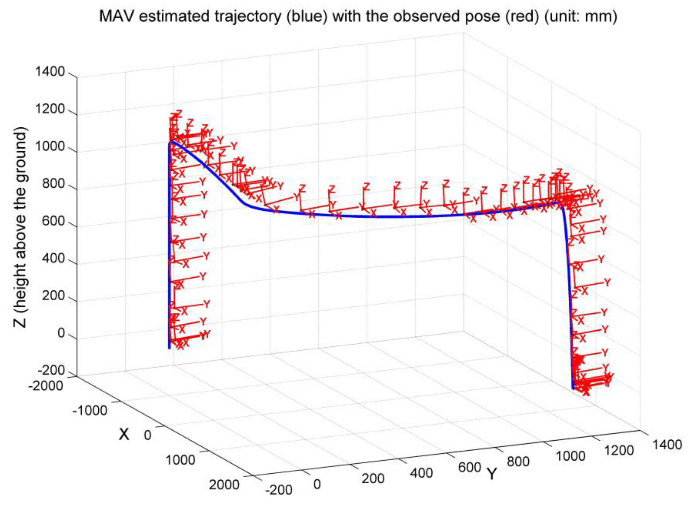
Meanwhile, another experiment of real-time pose estimation has also been carried out while the quadrotor is flying freely in a control region of the visual system. In this test, the position and heading of the quadrotor are remotely controlled by a ground station and its attitude is autonomously stabilized by the onboard IMU. The result of a part of the recovered flight trajectory estimated by the PF framework is shown in Figure 13. In order to be observed well, it should be noted that the Z-axis of the 3D world (inertial) frame has been converted to the opposite direction and points upwards.
From the results and discussion above, the proposed CVT enables a stable estimation when the flying quadrotor is within the view of the designed vision system. Additionally, the camera view or image noise may lead to different errors in each location method based on different constraints. It is helpful to achieve a stable result when the solutions from triangulation and P3P are referred to by a filter.
6. Conclusions
In summary, we have presented a combined vision technique and built a visual measurement system for MAV pose estimation. In this work, an indoor visual measurement system has been developed and introduced, including multi-camera parameter calibration, MAV detection, and design of a quadrotor. The unique contribution of this paper is the proposed CVT in which two visual positioning methods can be integrated in a PF framework to obtain a stable estimated pose. With the designed visual measurement system, some interesting proof-of-concept tests have been carried out. The results show that the proposed CVT can provide stable pose estimation for MAVs. In our future plan, the proposed system will be assembled into an on-ground navigation platform to guide the MAV for safe and precise landing. It can also be considered as a low-cost and high-performance flight test-bed, which can be applied to study the dynamics, control, and navigation of MAVs.
Acknowledgments
This work reported in this paper is the product of several research stages at the Wuhan University of Technology and has been sponsored in part by Natural Science Foundation of China (51579204), Double First-rate Project of WUT (472-20163042) and Graduate self-determined and innovative research Funds of WUT (2015-JL-014 and 2016IVA064). I thank three peer reviewers for their greatly appreciated comments and criticisms to help me improve my paper.
Author Contributions
H.Y. and C.X. conceived and designed the experiments; H.Y. and S.X. performed the experiments; Y.W. and C.Z. contributed the quadrotor platform and the experimental materials; H.Y. analyed the data; H.Y. and Q.L. wrote the paper.
Conflicts of Interest
The authors declare no conflict of interest.
References
- Sanchez-Lopez, J.L.; Pestana, J.; Saripalli, S.; Campoy, P. An Approach toward Visual Autonomous Ship Board Landing of a VTOL UAV. J. Intell. Robot. Syst. 2014, 74, 113–127. [Google Scholar] [CrossRef]
- Maza, I.; Kondak, K.; Bernard, M.; Ollero, A. Multi-UAV Cooperation and Control for Load Transportation and Deployment. J. Intell. Robot. Syst. 2010, 57, 417–449. [Google Scholar] [CrossRef]
- Mulgaonkar, Y.; Araki, B.; Koh, J.S.; Guerrero-Bonilla, L.; Aukes, D.M.; Makineni, A.; Tolley, M.T.; Rus, D.; Wood, R.J.; Kumar, V. The Flying Monkey: A Mesoscale Robot That Can Run, fly, and grasp. In Proceedings of the 2016 IEEE International Conference on Robotics and Automation (ICRA), Stockholm, Sweden, 16–21 May 2016. [Google Scholar]
- Brockers, R.; Humenberger, M.; Kuwata, Y.; Matthies, L.; Weiss, S. Computer Vision for Micro Air Vehicles. In Advances in Embedded Computer Vision; Springer: New York, NY, USA, 2014; pp. 73–107. [Google Scholar]
- Mondragón, I.F.; Campoy, P.; Martinez, C.; Olivares-Méndez, M.A. 3D pose estimation based on planar object tracking for UAVs control. In Proceedings of the IEEE International Conference on Robotics and Automation (ICRA), Anchorage, AK, USA, 3–7 May 2010. [Google Scholar]
- Gomez-Balderas, J.E.; Flores, G.; García Carrillo, L.R.; Lozano, R. Tracking a Ground Moving Target with a Quadrotor Using Switching Control. J. Intell. Robot. Syst. 2013, 70, 65–78. [Google Scholar] [CrossRef]
- Xu, G.; Qi, X.; Zeng, Q.; Tian, Y.; Guo, R.; Wang, B. Use of Land’s Coorperative Object to Estimate UAV’s Pose for Autonomous Landing. Chin. J. Aeronaut. 2013, 26, 1498–1505. [Google Scholar] [CrossRef]
- Shen, S.; Mulgaonkar, Y.; Michael, N.; Kumar, V. Vision-Based State Estimation for Autonomous Rotorcraft MAVs in complex Environments. In Proceedings of the IEEE International Conference on Robotics and Automation (ICRA), Karlsruhe, Germany, 6–10 May 2013. [Google Scholar]
- Chowdhary, G.; Johnson, E.N.; Magree, D.; Wu, A.; Shein, A. GPS-denied Indoor and Outdoor Monocular Vision Aided Navigation and Control of Unmanned Aircraft. J. Field Robot. 2013, 30, 415–438. [Google Scholar] [CrossRef]
- Weiss, S.; Achtelik, M.W.; Lynen, S.; Achtelik, M.C.; Kneip, L.; Chli, M.; Siegwart, R. Monocular Vision for Long-term Micro Aerial Vehicle State Estimation: A Compendium. J. Field Robot. 2013, 30, 803–831. [Google Scholar] [CrossRef]
- Yang, S.; Scherer, S.A.; Schauwecker, K.; Zell, A. Autonomous Landing of MAVs on an Arbitrarily Textured Landing Site Using Onboard Monocular Vision. J. Intell. Robot. Syst. 2014, 74, 27–43. [Google Scholar] [CrossRef]
- Thurrowgood, S.; Moore, R.J.; Soccol, D.; Knight, M.; Srinivasan, M.V. A Biologically Inspired, Vision-based Guidance System for Automatic Landing of a Fixed-wing Aircraft. J. Field Robot. 2014, 31, 699–727. [Google Scholar] [CrossRef]
- Herissé, B.; Hamel, T.; Mahony, R.; Russotto, F.X. Landing a VTOL Unmanned Aerial Vehicle on a Moving Platform Using Optical Flow. IEEE Trans. Robot. 2012, 28, 77–89. [Google Scholar] [CrossRef]
- Lupashin, S.; Hehn, M.; Mueller, M.W.; Schoellig, A.P.; Sherback, M.; D’Andrea, R. A Platform for Aerial Robotics Research and Demonstration: The Flying Machine Arena. Mechatronics 2014, 24, 41–54. [Google Scholar] [CrossRef]
- Michael, N.; Mellinger, D.; Lindsey, Q.; Kumar, V. The grasp multiple micro UAV testbed. IEEE Robot. Autom. Mag. 2010, 17, 56–65. [Google Scholar] [CrossRef]
- Valenti, M.; Bethke, B.; Fiore, G.; How, J.P. Indoor Multivehicle Flight Testbed for Fault Detection, Isolation and Recovery. In Proceedings of the AIAA Guidance, Navigation, and Control Conference and Exhibit, Keystone, CO, USA, 21–24 August 2006. [Google Scholar]
- How, J.; Bethke, B.; Frank, A.; Dale, D.; Vian, J. Real-time Indoor Autonomous Vehicle Test Environment. IEEE Control Syst. Mag. 2008, 28, 51–64. [Google Scholar] [CrossRef]
- Martínez, C.; Mondragón, I.F.; Olivares-Méndez, M.A.; Campoy, P. On-board and Ground Visual Pose Estimation Techniques for UAV Control. J. Intell. Robot. Syst. 2010, 61, 301–320. [Google Scholar] [CrossRef]
- Faessler, M.; Mueggler, E.; Schwabe, K.; Scaramuzza, D. A Monocular Pose Estimation System based on Infrared LEDs. In Proceedings of the IEEE International Conference on Robotics & Automation (ICRA), Hong Kong, China, 31 May–7 June 2014. [Google Scholar]
- Oh, H.; Won, D.Y.; Huh, S.S.; Shim, D.H.; Tahk, M.J.; Tsourdos, A. Indoor UAV Control Using Multi-Camera Visual Feedback. J. Intell. Robot. Syst. 2011, 61, 57–84. [Google Scholar] [CrossRef]
- Yoshihata, Y.; Watanabe, K.; Iwatani, Y.; Hashimoto, K. Multi-camera visual servoing of a micro helicopter under occlusions. Proceedings on the IEEE/RSJ International Conference on Intelligent Robots and Systems, San Diego, CA, USA, 29 October–2 November 2007. [Google Scholar]
- Altug, E.; Ostrowski, J.P.; Taylor, C.J. Control of A Quadrotor Helicopter Using Dual Camera Visual Feedback. Int. J. Robot. Res. 2005, 24, 329–341. [Google Scholar] [CrossRef]
- Jean-Yves Bouguet. Camera Calibration Toolbox for Matlab. 2008. Available online: http://www.vision.caltech.edu/bouguetj/calib_doc/index.html (accessed on 2 March 2015).
- Svoboda, T.; Martinec, D.; Pajdla, T. A convenientmulti-camera self-calibration for virtual environments. PRESENCE: Teleoper. Virtual Environ. 2005, 14, 407–422. [Google Scholar] [CrossRef]
- Lynen, S.; Achtelik, M.W.; Weiss, S.; Chli, M.; Siegwart, R. A Robust and Modular Multi-Sensor Fusion Approach Applied to MAV Navigation. In Proceedings of the IEEE/Rsj International Conference on Intelligent Robots and Systems (IROS), Tokyo, Japan, 3–7 November 2013. [Google Scholar]
- De Marina, H.G.; Pereda, F.J.; Giron-Sierra, J.M.; Espinosa, F. UAV Attitude Estimation Using Unscented Kalman Filter and TRIAD. IEEE Trans. Ind. Electron. 2012, 59, 4465–4475. [Google Scholar] [CrossRef]
- Gustafsson, F.; Gunnarsson, F.; Bergman, N.; Forssell, U.; Jansson, J.; Karlsson, R.; Nordlund, P.J. Particle Filters for Positioning, Navigation, and Tracking. IEEE Trans. Signal Process. 2002, 50, 425–438. [Google Scholar] [CrossRef]
Figure 1.
Structure diagram of the multi-camera measurement system.

Figure 2.
Multi-camera extrinsic calibration. (a) The waving bright spot in the camera view is detected; (b) recovery results of the camera structure and spot motion.
Figure 2.
Multi-camera extrinsic calibration. (a) The waving bright spot in the camera view is detected; (b) recovery results of the camera structure and spot motion.

Figure 3.
The MAV (micro aerial vehicle) system (a) and ground PC station (b).
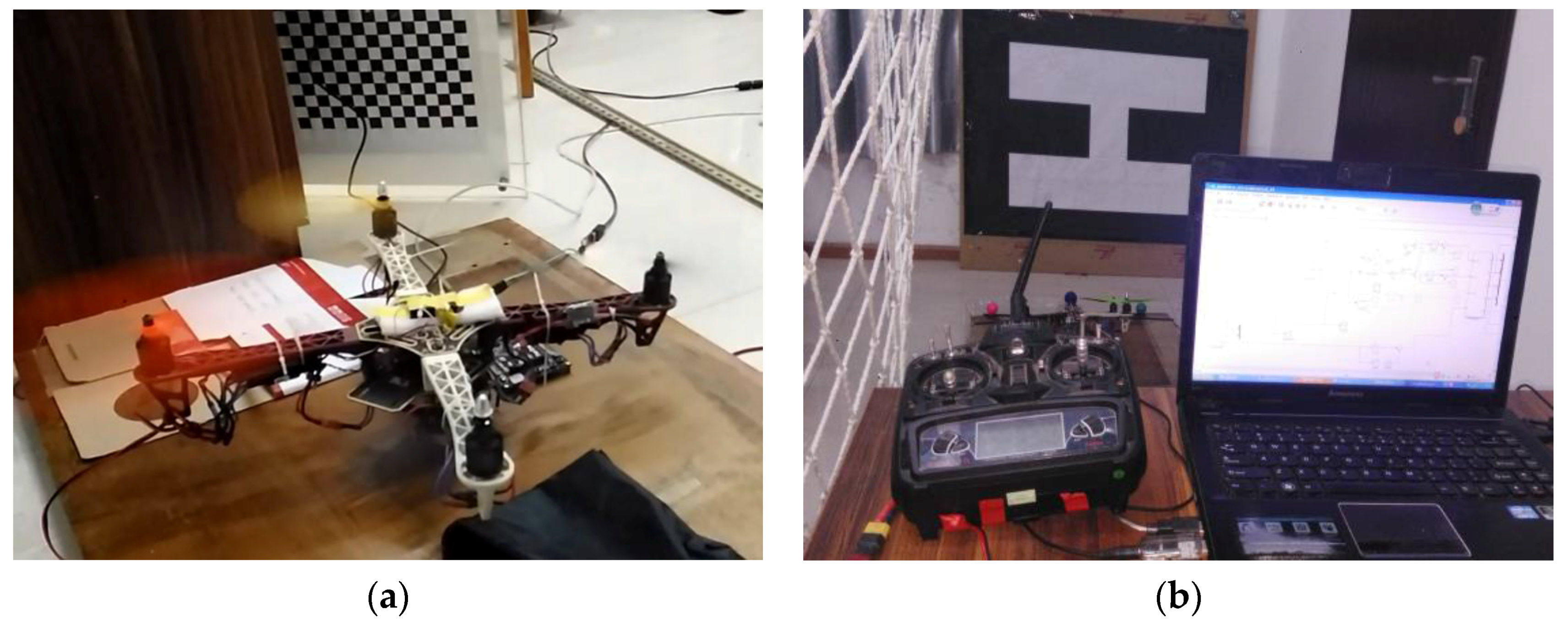
Figure 4.
Detection of one marker in two views. (a) marker detection and the corresponding epipolar line in one view; (b) marker detection and the corresponding epipolar line in the other view; (c) the image coordinates by continuous detection for the three markers in (a); (d) the image coordinates by continuous detection for the three markers in (b); (e) amplification of the green marker detection in (a).
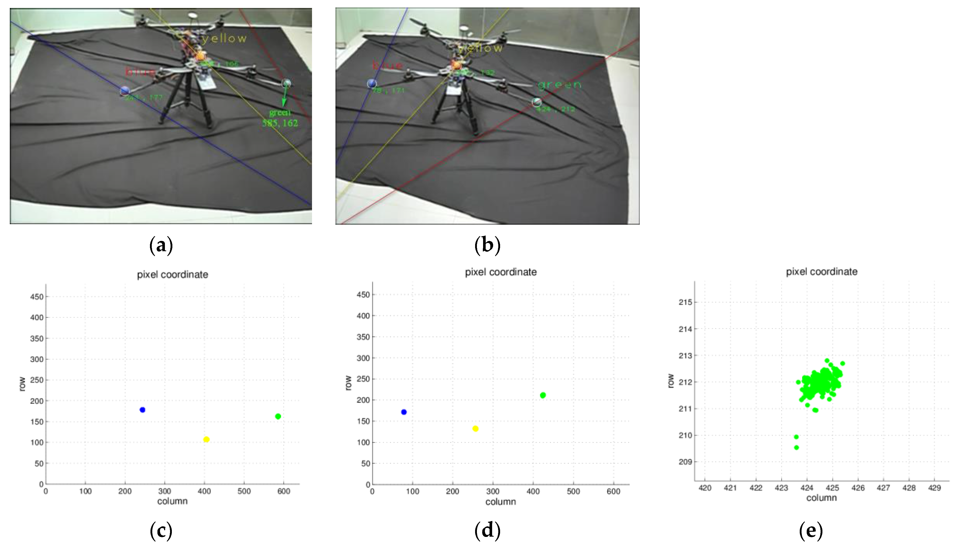
Figure 5.
(a) The multi-view triangulation method. (b) The mono-view P3P (perspective-three-point) method. (c) MAV pose computation.
Figure 5.
(a) The multi-view triangulation method. (b) The mono-view P3P (perspective-three-point) method. (c) MAV pose computation.
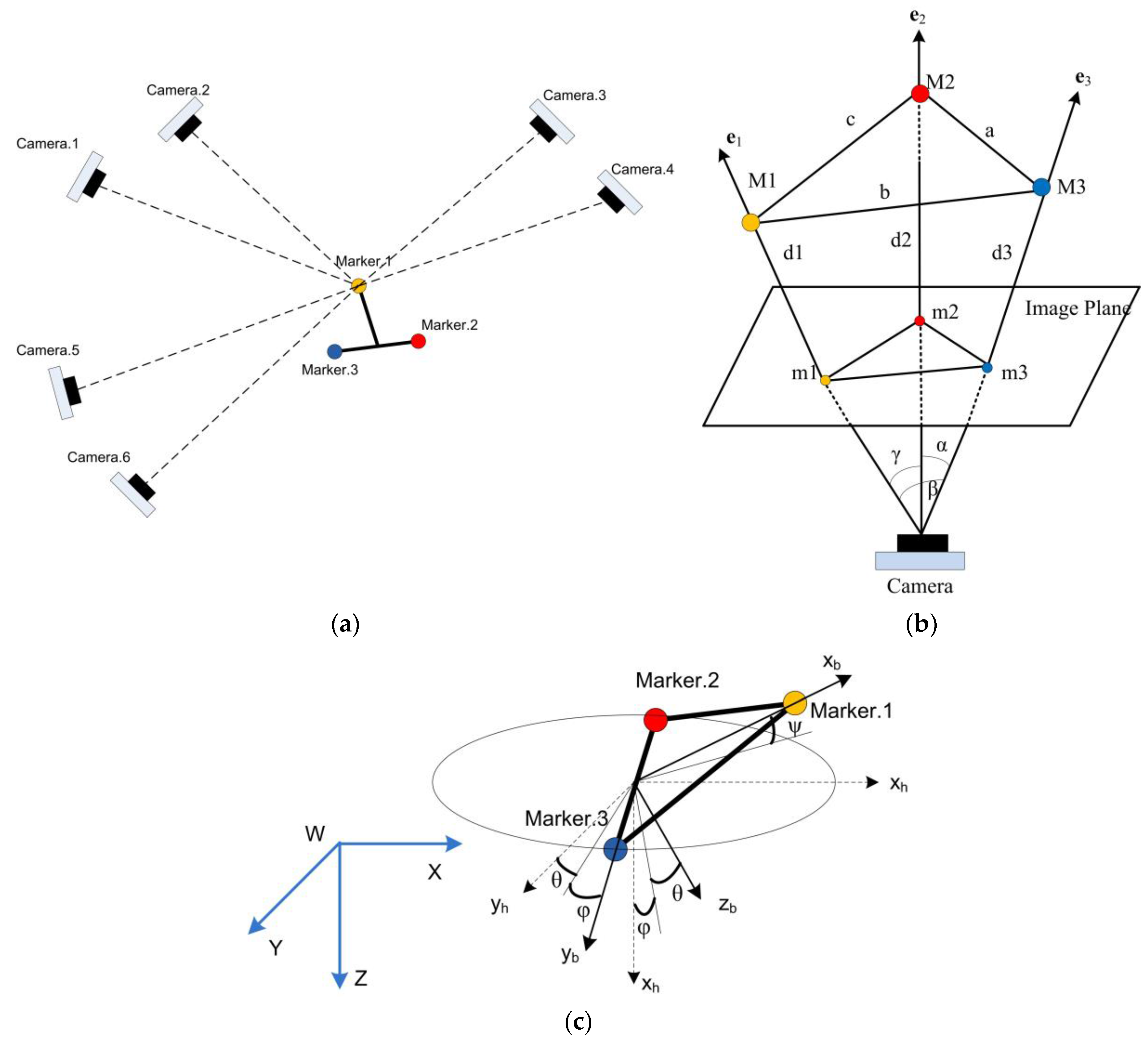
Figure 6.
State estimation based on multiple measurements from the visual system.
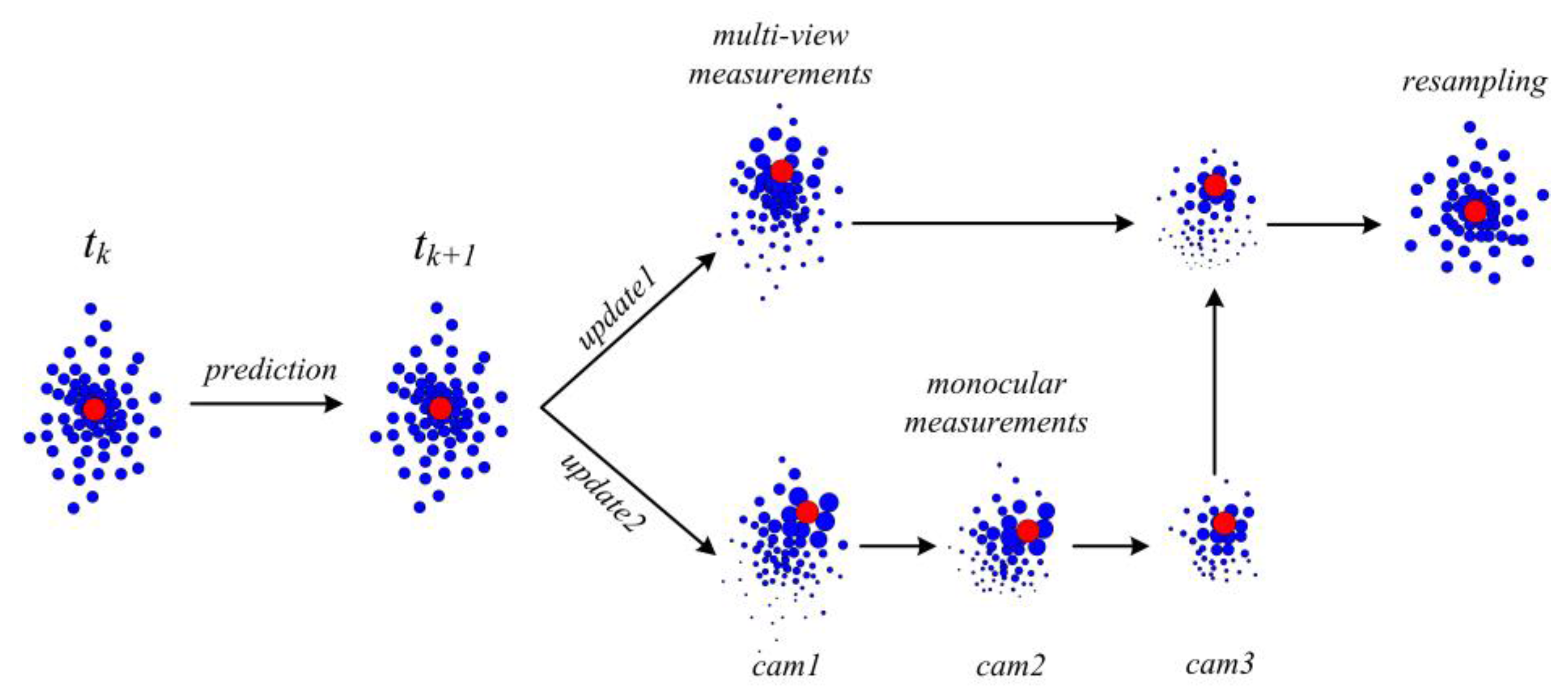
Figure 7.
The multi-camera measurement system and the testing MAV.
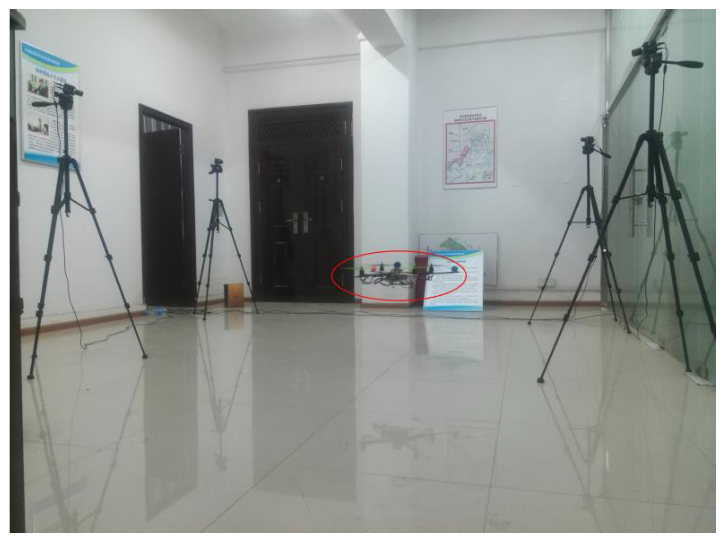
Figure 8.
Pose computation when the quadrotor keeps a fixed state. (A) Results of the multi-view triangulation method. (B) Results of the mono-view P3P method.
Figure 8.
Pose computation when the quadrotor keeps a fixed state. (A) Results of the multi-view triangulation method. (B) Results of the mono-view P3P method.

Figure 9.
Histograms of MAV at fixed orientation by the multi-view measurement.
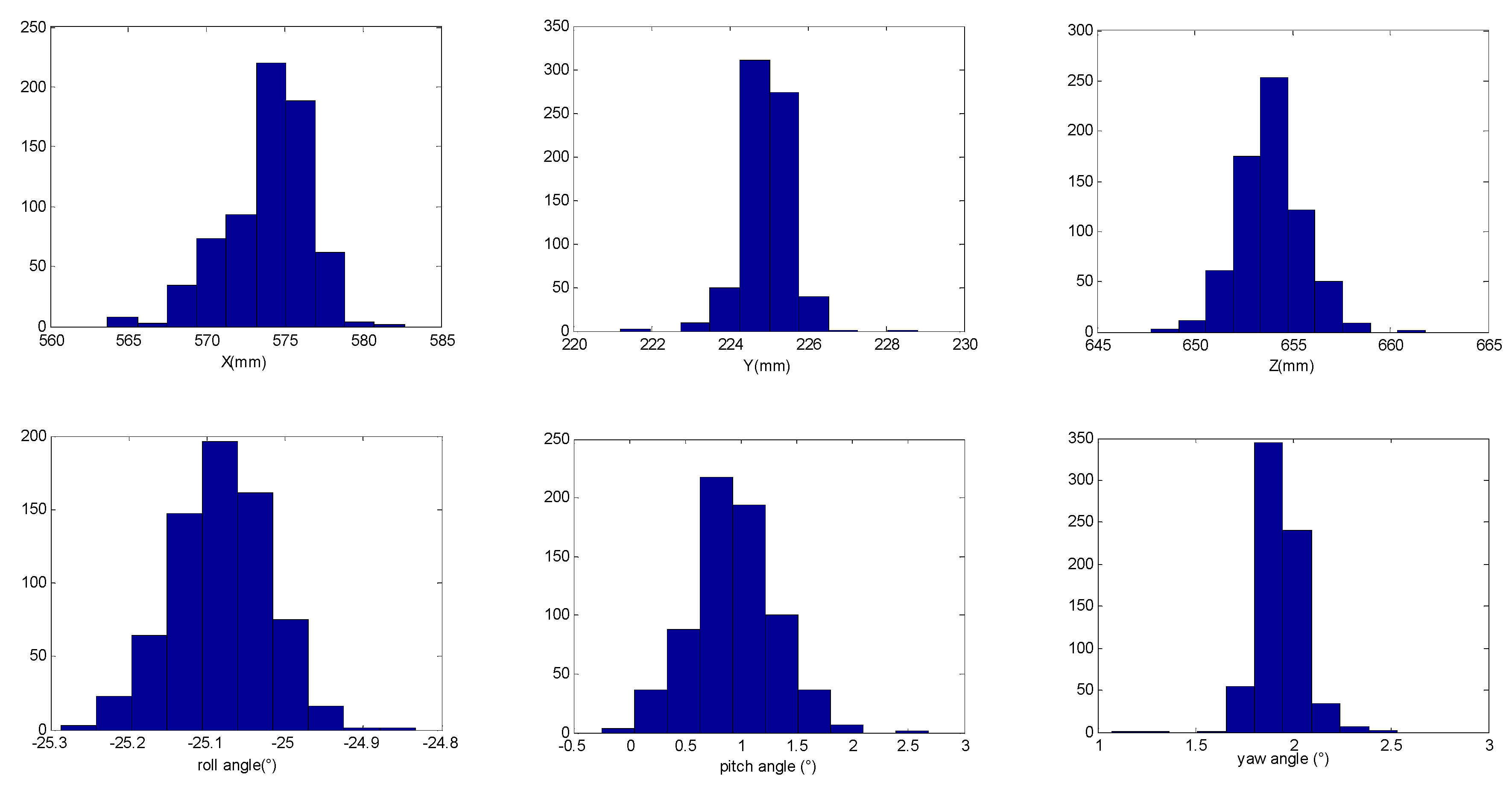
Figure 10.
Histograms of MAV at fixed orientation by the monocular measurement.

Figure 11.
MAV attitudes from visual (blue) and IMU (Inertial Measurement Unit) (red) measurements.

Figure 12.
MAV estimated state (blue) and observed measurements (red) from the visual system or IMU. (a) translational velocity in the inertial reference frame; (b) accelerated velocity in the body reference frame; (c) attitude angles in the inertial reference frame; (d) angular velocities in the body reference frame.
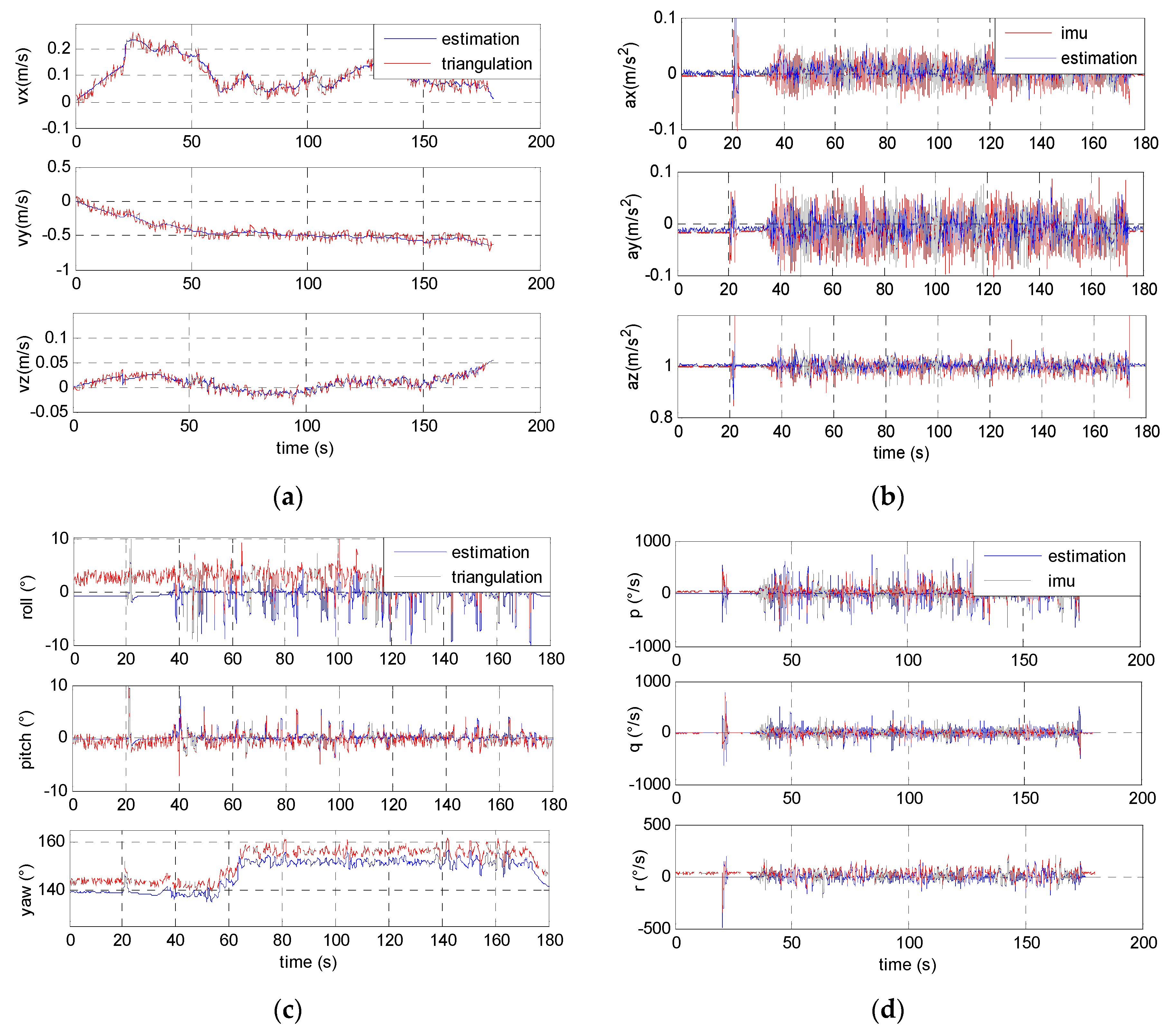
Figure 13.
Real time trajectory estimation (blue) and measurement pose (red) of the flying quadrotor in the 3D reference frame.
Figure 13.
Real time trajectory estimation (blue) and measurement pose (red) of the flying quadrotor in the 3D reference frame.
© 2017 by the authors. Licensee MDPI, Basel, Switzerland. This article is an open access article distributed under the terms and conditions of the Creative Commons Attribution (CC BY) license (http://creativecommons.org/licenses/by/4.0/).
Share and Cite
MDPI and ACS Style
Yuan, H.; Xiao, C.; Xiu, S.; Wen, Y.; Zhou, C.; Li, Q. A New Combined Vision Technique for Micro Aerial Vehicle Pose Estimation. Robotics 2017, 6, 6. https://doi.org/10.3390/robotics6020006
AMA Style
Yuan H, Xiao C, Xiu S, Wen Y, Zhou C, Li Q. A New Combined Vision Technique for Micro Aerial Vehicle Pose Estimation. Robotics. 2017; 6(2):6. https://doi.org/10.3390/robotics6020006
Chicago/Turabian StyleYuan, Haiwen, Changshi Xiao, Supu Xiu, Yuanqiao Wen, Chunhui Zhou, and Qiliang Li. 2017. "A New Combined Vision Technique for Micro Aerial Vehicle Pose Estimation" Robotics 6, no. 2: 6. https://doi.org/10.3390/robotics6020006
Note that from the first issue of 2016, this journal uses article numbers instead of page numbers. See further details here.