Automated Assembly Using 3D and 2D Cameras

Department of Mechanical and Industrial Engineering, Norwegian University of Science and Technology, N-7491 Trondheim, Norway
*
Author to whom correspondence should be addressed.
†
These authors contributed equally to this work.
Robotics 2017, 6(3), 14; https://doi.org/10.3390/robotics6030014
Submission received: 31 March 2017
/
Revised: 20 May 2017
/
Accepted: 19 June 2017
/
Published: 27 June 2017
(This article belongs to the Special Issue Robotics and 3D Vision)
Abstract
:2D and 3D computer vision systems are frequently being used in automated production to detect and determine the position of objects. Accuracy is important in the production industry, and computer vision systems require structured environments to function optimally. For 2D vision systems, a change in surfaces, lighting and viewpoint angles can reduce the accuracy of a method, maybe even to a degree that it will be erroneous, while for 3D vision systems, the accuracy mainly depends on the 3D laser sensors. Commercially available 3D cameras lack the precision found in high-grade 3D laser scanners, and are therefore not suited for accurate measurements in industrial use. In this paper, we show that it is possible to identify and locate objects using a combination of 2D and 3D cameras. A rough estimate of the object pose is first found using a commercially available 3D camera. Then, a robotic arm with an eye-in-hand 2D camera is used to determine the pose accurately. We show that this increases the accuracy to mm and . This was demonstrated in a real industrial assembly task where high accuracy is required.
1. Introduction
Computer vision is frequently used in industry to increase the flexibility of automated production lines without reducing the efficiency and high accuracy that automated production requires.
Assembly applications benefit from computer vision in many ways. Production lines with frequent changeovers, which occurs in some industries, can benefit from computer vision to determine position and orientation of the parts on the production line, without the need of additional equipment [1]. Assembly production lines are mostly a very controlled and structured environment, which is suitable for computer vision methods, to make them perform more predictably [2].
Shadows and reflections are frequent problems in 2D computer vision [3], since the methods will yield different results if an object is viewed from different angles or if its orientation changes. The key to gaining accurate and predictable results is to have a good initial position of the camera relative to the object. 2D eye-in-hand cameras [4] can actively change the viewpoint of a camera to a scene. This makes it possible to view an object from a particular angle, no matter which orientation it has. By using an eye-in-hand camera in this way, more predictable results can be achieved than with a stationary camera. However, in order to do this, the camera must be moved to suitable position relative to the object, which has to be found first.
The rising use of 3D cameras gives the opportunity for different methods and approaches [5], mostly due to the availability of depth information, which makes it easier to determine properties such as shapes and occlusion, compared to a traditional 2D camera. However, commercially available 3D cameras lack precision, which can only be found in high-grade 3D laser scanners [6], leading to inaccurate measurements that are not sufficiently accurate for automated production. By using the 3D camera to detect objects and determine a rough estimate of their position, the eye-in-hand camera can use these estimates to move to a suited initial position.
Within computer vision, there are several approaches on how to detect, classify and estimate poses of objects, both within 2D and 3D computer vision. Examples of these are voting-based algorithms, such as [7], human robot collaboration, such as [8], and probabilistic methods, such as [9]. However, these approaches focus more on successful recognition and computation time rather than accuracy of the pose estimation. This makes them ideal for pick and place algorithms such as [10], but not for accurate assembly tasks.
In this paper, we combine existing solutions from both 2D eye-in-hand and 3D computer vision in order to detect objects more predictably and with higher accuracy than either 3D or 2D methods separately. This system uses the Computer Aided Design (CAD) model of each object to render 3D views [11] and use these to determine the position and orientation of each object with sufficient accuracy to be able to assemble the objects using a robotic arm.
This paper is organized as follows. First, a brief presentation is given of some common computer vision methods that are used in the paper, followed by a description of the system that uses both 2D and 3D computer vision methods. Finally, the paper provides experimental results of an assembly task using one 3D camera, one eye-in-hand 2D camera and two robotic arms.
2. Preliminaries
In the paper, a point cloud is a set of points , represented by Euclidean vectors, so that
RANSAC [12] is short for Random Sample Consensus and is an iterative method for estimating model parameters from a data set containing several outliers. Figure 1a shows a scene consisting of three objects placed on a table. The table is detected in Figure 1b using RANSAC with a plane estimation. The inliers are marked in light gray. Figure 1c shows the scene when the inliers have been removed.
The Iterative Closest Point (ICP) algorithm [13,14] is an iterative method for aligning two sets of point clouds. This is done by minimizing the distance between corresponding points.
One method that is suitable for calculating the rotation and translation is by using Singular Value Decomposition (SVD) to minimize the least squares error [15].
The scale invariant feature transform (SIFT) [16] is a method for matching image features. The method searches through images for interest points, which are points in an image surrounded by areas with sufficient information that makes it possible to distinguish them. The algorithm computes a SIFT descriptor for the image interest points, which is a histogram that can be used for matching.
3. Approach
The approach in this paper takes in a set of 3D CAD models and searches for these models within a scene. The system is divided into a 3D object detection system and a 2D object alignment system, as seen in Figure 2. The 3D detection system takes a 3D image and compares it to the given CAD models. The system identifies each object and calculates a rough estimate of the position and orientation of them. The estimates are then used as input to a 2D alignment system, where a 2D camera is mounted on a robotic arm, and uses 2D computer vision approaches to get a fine estimate of the positions and orientations of each object.
3.1. 3D Object Detection
3.1.1. Viewpoint Sampling
A point cloud of a CAD model includes points on all sides of the 3D object, while a point cloud that forms a 3D camera will only have points on the part of the object, which is seen from the 3D camera.
To compare a point cloud captured by a 3D camera and a CAD model, it is important to make a comparison to the CAD model when viewed from the view point of the 3D camera. To do this, virtual 3D images of the object is generated from a CAD model from a selection of different viewpoints. Figure 3 shows a sample of the generated point clouds for an automotive part seen from seven different viewpoints.
Viewpoints are calculated using a tessellated sphere that is fit around the CAD model. Then, one viewpoint is rendered for each vertex of the tessellated sphere, and a point cloud is generated from each viewpoint.
3.1.2. Removing Unqualified Points
The 3D camera will capture the whole scene. The resulting 3D image will include the objects, and in addition, points representing the foreground, background and the table where the objects are placed. In order to minimize the search area for the algorithms, the points that do not represent the object should be removed. The first step of removing unqualified points is to remove points outside a specified range. Since the objects are placed on a table, all points that are outside of the bounds of the table can safely be removed, see Figure 4.
When these points are removed, the majority of the points in the point cloud will represent the table. The points representing the objects are on top of the table. This means that, by estimating the table plane, all points above this plane will represent the objects, while the points on the plane or under will be unqualified points. Since most of the point cloud has points representing the table, RANSAC can be used for estimating this plane.
A plane is determined by three points , and in the plane. Then, the normal of the plane, is
and the distance from the origin is
A point will have the distance to the plane, where when the point is in the direction of the normal of the plane.
To generate the model candidate for a plane in each iteration of RANSAC, three random points from the point cloud are picked: , and . The candidate is then compared to the point cloud data to determine which points in the point cloud are inliers and which are outliers.
A point can be considered an inlier to the estimated plane if
where is the given point, and is a user-specified distance threshold. This threshold is the maximum distance away from the plane, where a point can be considered an inlier. All points outside of this threshold are considered outliers.
When the RANSAC algorithm is finished, the optimal plane estimate is found, and the inlier points of the plane are determined. With this information, the inlier points of the plane can be removed from the 3D image, as these represent the table and not the objects on top. In addition, the points below the table, which are characterized by , can also be removed.
3.1.3. Object Detection
The remaining points in the point cloud will be part of an object or noisy outliers. In order to detect the objects, a region growing algorithm is used.
The region growing method finds points that are in close proximity and group them together. This is possible because the distance between two points on different objects are large relative to the distance between two points on the same object.
This algorithm results in one large group for each object in addition to several smaller groups containing noisy points. These smaller groups can be eliminated, based on their small size.
One new point cloud is then created for each of the remaining large groups. Each of these point clouds are the representation of an object on the table.
3.1.4. Object Alignment
From the previous step, there will be a number of point clouds, each representing an object on the table. It is not known which point cloud corresponds to each object, nor their position or orientation.
The next step is to find the viewpoint of the CAD models that best matches the point cloud for a particular object, which will give a rough estimate of position and orientation as well as the most likely identity of the object.
This is done by generating Fast Point Feature Histogram (FPFH) and Viewpoint Feature Histograms (VFH) descriptors for the point clouds of each object, and comparing these to viewpoint point clouds generated from the CAD models using the Sample Consensus-Initial Alignment (SAC-IA) [17] method.
SAC-IA uses the FPFH and VPF of each point cloud and their corresponding viewpoint point cloud to get the initial alignment of the object. SAC-IA is short for Sample Consensus Initial Alignment and is a variant of ICP that searches on a global scale rather than on a local scale as ICP does. This results in finding the viewpoint point cloud that best matches each object as well as the alignment between the viewpoint point cloud and the object point cloud.
The alignment from the SAC-IA method is a rough estimate, so the final step is to use ICP on the point clouds, resulting in an estimate of the alignment of each object in respect to the camera.
3.2. 2D Object Alignment
Due to the hardware limitations of the 3D-camera, the alignment estimates does not satisfy the requirements for assembly, so further estimations are required.
By placing a 2D-camera at the end-effector of a robotic arm (see Figure 5), the camera can be moved over each object and fine-tune their position and orientation. The robotic arm is positioned to a point right over the estimate calculated from the 3D computer vision system. This makes the camera be located approximately above the center of the object, and the camera can view the top of the object.
A 2D reference image is provided for each object, showing the top of the object, see Figure 6. When the 2D camera captures an image, it can be compared to the reference image using the SIFT method. The homography between the matched points is found, which makes it possible to find the transform between the reference image and the captured image. The reference image depicts the object in the center and at 0°, which means that the rotation of the homography is the orientation of the object, while the translation is the fine estimate of the position. This calculation can be run several times to converge to a better result, or to verify the current estimate:
A sample from one of the experiments can be seen in Figure 7.
4. Experiments and Results
4.1. Setup
Tests of the assembly operation using the presented object detection procedures were performed in a robotic laboratory. The robotic cell was equipped with the following hardware:
- Two KUKA KR 6 R900 sixx (KR AGILUS) six-axis robotic manipulators (Augsburg, Germany).
- Microsoft Kinect™ One 3D depth sensor (Redmond, WA, USA).
- Logitech C930e web camera (Lausanne, Switzerland).
- Schunck PSH 22-1 linear pneumatic gripper (Lauffen, Germany).
Software used:
- Ubuntu 14.04 (Canonical, London, United Kindom).
- Point Cloud Library 1.7 (Willow Garage, Menlo Park, CA, USA).
- OpenCV 3.1 (Intel Corpiration, Santa Clara, CA, USA).
- Robot Operating System (ROS) Indigo (Willow Garage, Menlo Park, CA, USA).
The setup is shown in Figure 8. The pneumatic gripper was mounted at one of the robotic manipulators, while the web camera was mounted at the second manipulator. The Kinect One 3D camera was mounted behind the table and tilted towards the table top so that it could view the parts placed on the table. The position of the camera was calibrated in reference to the world frame of the robotic cell.
The assembly of two automotive parts was investigated in the experiment. These parts are shown in Figure 9.
A total of three different experiments were conducted to study the performance of a two-step alignment with initial 3D alignment and final 2D alignment. The first experiment was performed to determine the accuracy of the Kinect One 3D camera for the initial alignment, and the second experiment was to determine the accuracy of the 2D camera that was used in the final alignment. The last experiment was a full assembly of the two test objects using both 3D and 2D vision.
4.2. Experiment 1: 3D Accuracy
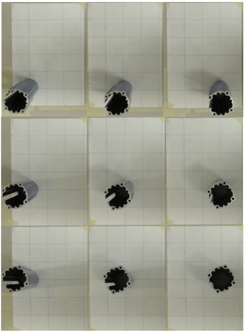
The first experiment was designed to determine the accuracy of the 3D object detection system. The two objects of interest were positioned on the table in known locations. A grid of 5 cm × 5 cm squares was used to manually determine position the objects, as shown in Figure 10. The experiment was conducted 10 times on 16 different positions, and the resulting position from the 3D detection system was compared to the actual position. This was done with both of the objects.
4.2.1. Results
The experiment described above allowed the accuracy of the 3D detection procedure to be evaluated.
The test results show that the following positional deviations from the actual objects are shown in Table 1, Table 2, Table 3 and Table 4.
The test results for the initial alignment show that the maximum positional error from the 3D measurements for both the x- and y-axis is below cm. This is acceptable as a first step to make it possible to perform a final 2D alignment to achieve the required industrial accuracy.
4.3. Experiment 2: 2D Stability
The accuracy of a 2D computer vision method is related to the stability of the object detection, and this is directly related to the amount of good and repeatable keypoints detected in the reference and captured 2D image. If the detected keypoints differ every time an image is captured, the homography matrix computed from the feature correspondences will influence the computation of the object orientation significantly.
In order to ensure that this will not be a restricting factor in the assembly operation, an experiment was performed. The experiment was performed by positioning the object of interest at the table with two given orientations, 0° and 90°. The manipulator with the 2D camera in an eye-in-hand arrangement was moved to a distance from the object along the z-axis empirically chosen based on the rate of successful matching using SIFT. The detected object center is then aligned with the camera optical center. For every object, the angle of orientation was calculated based on the results of the 2D vision methods. This was done every time the camera captured an image. The mean was calculated for 10 measurements until the data set consists of 25 data points. The difference in degrees between minimum and maximum orientation estimates were used to determine the accuracy of the system.
The stability was first tested using SIFT, and it was then compared to using a hybrid algorithm, where SIFT keypoints were used with the Speeded Up Robust Feature (SURF) descriptor [18].
4.3.1. Results
It is evident from these results that the orientation of object A is the hardest to detect with certainty. Detection of object B is much more stable. This also shows that, using the SIFT method, one can acquire an accuracy of . The mean error was , which is acceptable for assembly.
4.4. Experiment 3: Full Assembly
Based on the results from the previous experiments, a full assembly operation was be performed in an experiment. The procedure if the experiment was as follows:
- Place the two objects to be assembled at random positions and orientations on the table.
- Run the initial 3D alignment described in described in Section 3.
- Perform the final 2D alignment by moving the robot in position above the part found in the initial alignment.
- Move the robotic manipulator with the gripper to the estimated position of the first part, and pick it up. The manipulator then moved the part to the estimated pose of the second part to assemble the two parts.
These three steps were repeated for 10 unique assembly operations. The assembly operations are only considered as a success if the parts could be assembled without the use of force. An overview is shown in Figure 11.
4.4.1. Results
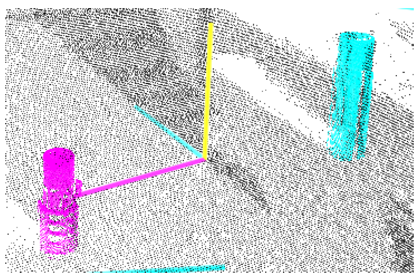
The assembly experiment is performed for 10 unique positions and orientations of object A and object B as described in Section 4.4. One of the 3D object detection results are visualized in Figure 12, while one of the results from the 2D object alignment is shown in Figure 13.
Correction of the object position is performed using the 2D object detection and aligns the object center with the camera optical center as illustrated in Figure 14. The robotic end-effector pose is retrieved in world coordinates and the orientation is calculated.
With the acquired position and orientation of both objects, a pick and place operation can be performed. In seven out of 10 assembly operations, the objects were successfully assembled, with an accuracy lower than 1 mm in position and 1° in orientation. In the remaining three attempts, the orientation of object A was the limiting factor. Typically, the failure was caused by situations as illustrated in Figure 15a, where a marginal error in orientation acquisition would prevent further execution of the assembly operation. This error was both due to the lack of accuracy in the 2D computer vision system and the gripping action, which displaced the orientation of the object.
A video of the method and conducted experiment can be downloaded at [19].
5. Discussion
Experiment 1 describes the accuracy of the 3D Detection system, while Experiment 2 describes the accuracy of the 2D Alignment system.
Experiment 1 concludes that the accuracy does not meet the requirements of the assembly task, since it shows that the maximum error was 1.96 cm, while the requirement was less than 1 mm. This, however, does meet the requirements for performing 2D alignment.
Experiment 2 concluded that the 2D alignment meets the requirements of the assembly, which is below 1°. These results are assuming that the camera is watching the object from the top, which is possible given the rough position estimate from the 3D Detection system.
Experiment 3 concludes that combining a 2D and 3D vision system, where both systems lack sufficient accuracy, can achieve said accuracy if combined.
In the experiment, it is assumed that the objects that are to be detected are not occluded and that they are standing so that the top of the object is always facing upwards. The given case assumes that the objects are properly aligned on the table, and that any irregularities, such as a fallen over or missing object, does not occur.
An extension of the system where the 2D camera can move more freely and view the object from different sides will be able to handle the special cases, where an object has an irregular alignment.
6. Conclusions
The 3D detection method resulted in an estimate with roughly 2 cm accuracy. By combining this with the 2D eye-in-hand camera to fine-tune the estimates, the accuracy was corrected to 1 mm in position and 1° in orientation. The results obtained from testing the full solution shows that such a detection system is viable in an automated assembly application.
Acknowledgments
There were no funding for the study.
Author Contributions
A.B., A.L.K. and K.L. conceived and designed the experiments; A.B. and K.L. performed the experiments; A.B. and K.L. analyzed the data; A.L.K. and O.E. contributed reagents/materials/analysis tools; A.L.K. wrote the paper.
Conflicts of Interest
The authors declare no conflict of interest.
References
- Dietz, T.; Schneider, U. Programming System for Efficient Use of Industrial Robots for Deburring in SME Environments. In Proceedings of the 7th German Conference on Robotics ROBOTIK 2012, Munich, Germany, 21–22 May 2012; pp. 428–433. [Google Scholar]
- Freeman, W.T. Where computer vision needs help from computer science. In Proceedings of the ACM-SIAM Symposium on Discrete Algorithms (SODA), San Francisco, CA, USA, 23–25 January 2011; pp. 814–819. [Google Scholar]
- Blake, A.; Brelstaff, G. Geometry from Specularities. In Proceedings of the Second International Conference on Computer Vision, Tampa, FL, USA, 5–8 December 1988. [Google Scholar]
- Chaumette, F.; Hutchinson, S.A. Visual Servo Control, Part II: Advanced Approaches. IEEE Robot. Autom. Mag. 2007, 14, 109–118. [Google Scholar] [CrossRef]
- Campbell, R.J.; Flynn, P.J. A Survey of Free-Form Object Representation and Recognition Techniques. Comput. Vis. Image Underst. 2001, 210, 166–210. [Google Scholar] [CrossRef]
- Khoshelham, K. Accuracy Analysis of Kinect Depth Data. Int. Arch. Photogramm. Remote Sens. Spat. Inf. Sci. 2012, XXXVIII-5, 133–138. [Google Scholar] [CrossRef]
- Nguyen, D.D.; Ko, J.P.; Jeon, J.W. Determination of 3D object pose in point cloud with CAD model. In Proceedings of the 2015 21st Korea-Japan Joint Workshop on Frontiers of Computer Vision, Mokpo, Korea, 28–30 January 2015. [Google Scholar]
- Luo, R.C.; Kuo, C.W.; Chung, Y.T. Model-based 3D Object Recognition and Fetching by a 7-DoF Robot with Online Obstacle Avoidance for Factory Automation. In Proceedings of the IEEE International Conference on Robotics and Automation, Seattle, WA, USA, 26–30 May 2015; Volume 106, pp. 2647–2652. [Google Scholar]
- Lutz, M.; Stampfer, D.; Schlegel, C. Probabilistic object recognition and pose estimation by fusing multiple algorithms. In Proceedings of the IEEE International Conference on Robotics and Automation, Karlsruhe, Germany, 6–10 May 2013; pp. 4244–4249. [Google Scholar]
- Rennie, C.; Shome, R.; Bekris, K.E.; De Souza, A.F. A Dataset for Improved RGBD-Based Object Detection and Pose Estimation for Warehouse Pick-and-Place. IEEE Robot. Autom. Lett. 2016, 1, 1179–1185. [Google Scholar] [CrossRef]
- Aldoma, A.; Vincze, M.; Blodow, N.; Gossow, D.; Gedikli, S.; Rusu, R.B.; Bradski, G. CAD-model recognition and 6DOF pose estimation using 3D cues. In Proceedings of the IEEE International Conference on Computer Vision, Barcelona, Spain, 6–13 November 2011; pp. 585–592. [Google Scholar]
- Schnabel, R.; Wahl, R.; Klein, R. Efficient RANSAC for point-cloud shape detection. Comput. Graph. Forum 2007, 26, 214–226. [Google Scholar] [CrossRef]
- Chen, Y.; Medioni, G. Object modeling by registration of multiple range images. In Proceedings of the 1991 IEEE International Conference on Robotics and Automation, Sacramento, CA, USA, 9–11 April 1991; Volume 10, pp. 2724–2729. [Google Scholar]
- Besl, P.; McKay, N. A Method for Registration of 3-D Shapes. Int. Soc. Opt. Photonics 1992, 586–606. [Google Scholar] [CrossRef]
- Arun, K.S.; Huang, T.S.; Blostein, S.D. Least-squares fitting of two 3-D point sets. IEEE Trans. Pattern Anal. Mach. Intell. 1987, 5, 698–700. [Google Scholar] [CrossRef]
- Lowe, D.G. Distinctive Image Features from Scale-Invariant Keypoints. Int. J. Comput. Vis. 2004, 60, 91–110. [Google Scholar] [CrossRef]
- Rusu, R.B.; Blodow, N.; Beetz, M. Fast Point Feature Histograms (FPFH) for 3D registration. In Proceedings of the IEEE International Conference on Robotics and Automation, Kobe, Japan, 12–17 May 2009; pp. 3212–3217. [Google Scholar]
- Bay, H.; Tuytelaars, T.; Gool, L.V. Surf: Speeded up robust features. In Proceedings of the European Conference on Computer Vision, Graz, Austria, 7–13 May 2006. [Google Scholar]
- Kleppe, A.L.; Bjørkedal, A.; Larsen, K.; Egeland, O. Website of NTNU MTP Production Group. Available online: https://github.com/ps-mtp-ntnu/Automated-Assembly-using-3D-and-2D-Cameras/ (accessed on 31 March 2017).
Figure 1.
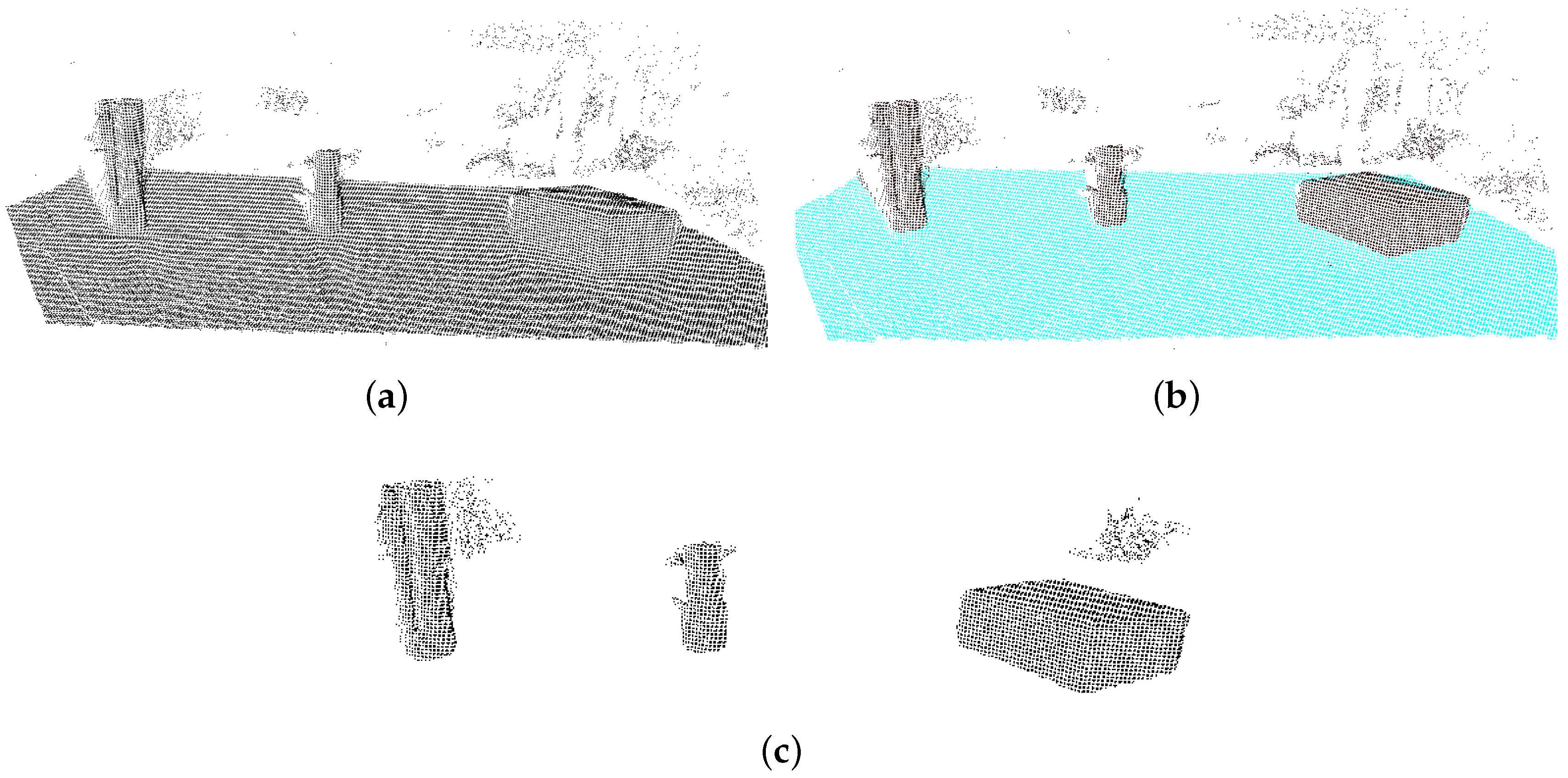
The RANSAC method performed on a table with objects. (a) A scene with multiple objects placed on a table; (b) the table surface is detected using RANSAC. The cyan points are inliers of the plane estimate; (c) The scene after removing the inliers, resulting in only the points representing the three objects.
Figure 1.
The RANSAC method performed on a table with objects. (a) A scene with multiple objects placed on a table; (b) the table surface is detected using RANSAC. The cyan points are inliers of the plane estimate; (c) The scene after removing the inliers, resulting in only the points representing the three objects.

Figure 2.
Overview of the flow of the system. It can be seen that the 3D Detection System calculates a rough position estimate given a set of CAD models, and this is fed into the 2D Alignment System, resulting in a fine position and orientation estimate.
Figure 2.
Overview of the flow of the system. It can be seen that the 3D Detection System calculates a rough position estimate given a set of CAD models, and this is fed into the 2D Alignment System, resulting in a fine position and orientation estimate.
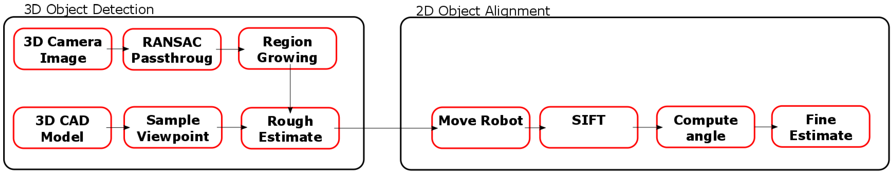
Figure 3.
Point clouds of the same object seen from different viewpoints generated from a CAD model of the object.
Figure 3.
Point clouds of the same object seen from different viewpoints generated from a CAD model of the object.
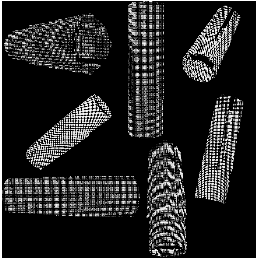
Figure 4.
Before and after pictures of removing foreground and background points. (a) Raw point cloud captured by the 3D camera; (b) Image after removing unwanted points, which are the points outside the bounds of the table.
Figure 4.
Before and after pictures of removing foreground and background points. (a) Raw point cloud captured by the 3D camera; (b) Image after removing unwanted points, which are the points outside the bounds of the table.
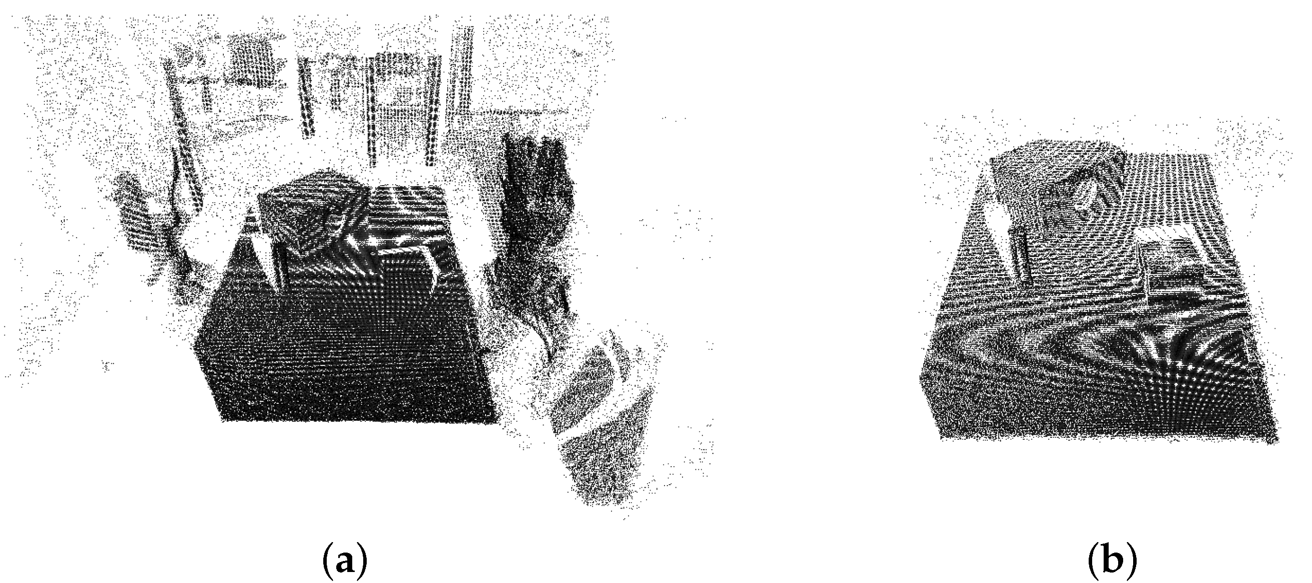
Figure 5.
Overview of the 2D camera setup. It can be seen that the camera is placed at the end-effector of the robot, and it is pointing downward.
Figure 5.
Overview of the 2D camera setup. It can be seen that the camera is placed at the end-effector of the robot, and it is pointing downward.
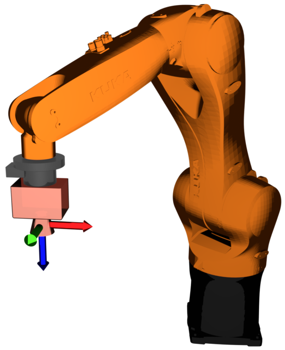
Figure 6.
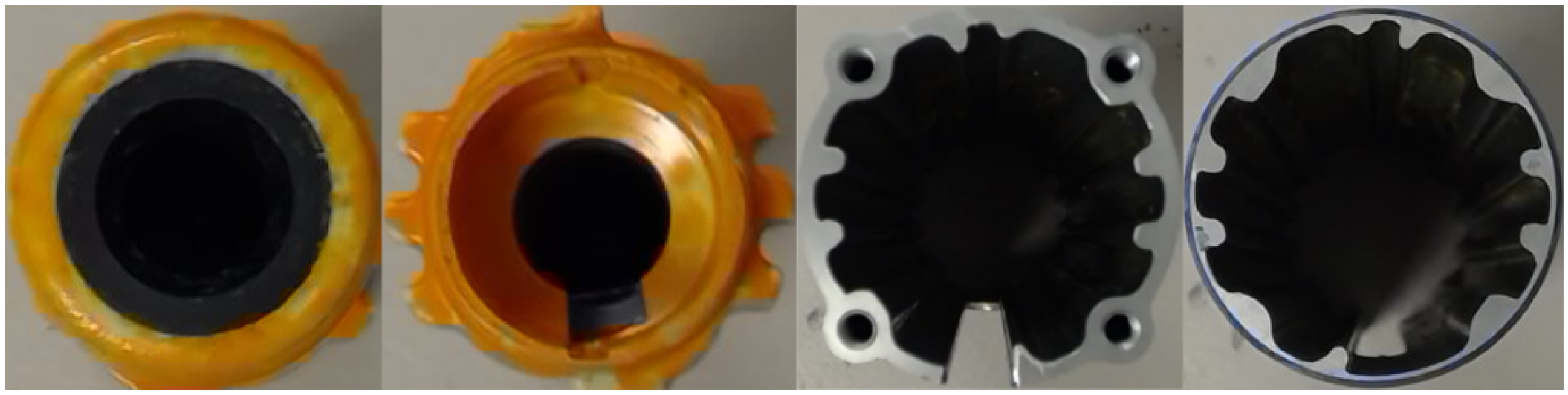
Reference images for each object. From left to right: The top of object A, the bottom of object A, the top of object B, the bottom of object B.
Figure 6.
Reference images for each object. From left to right: The top of object A, the bottom of object A, the top of object B, the bottom of object B.

Figure 7.
The green rectangle is the position of the reference image found in the captured image. The green circle is the current rough estimate from the 3D object detection system, while the red circle is the fine estimate of the position. The blue circles are the descriptors found with the SIFT method.
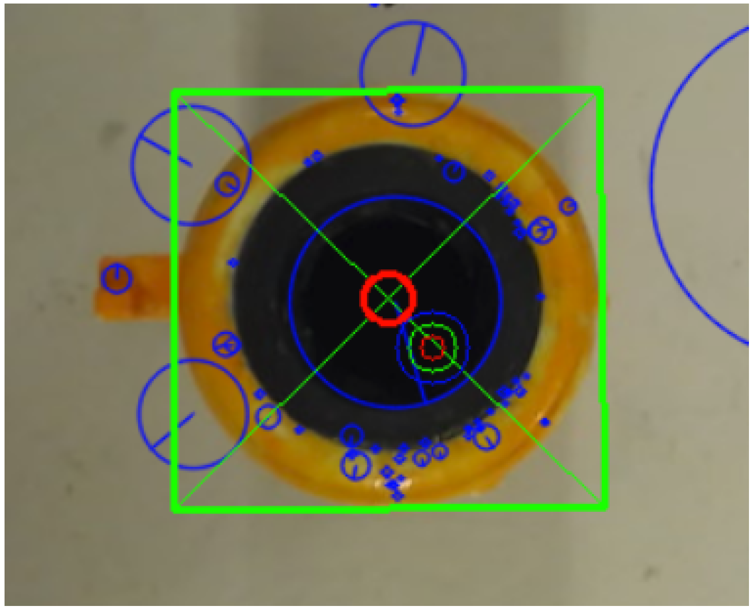
Figure 8.
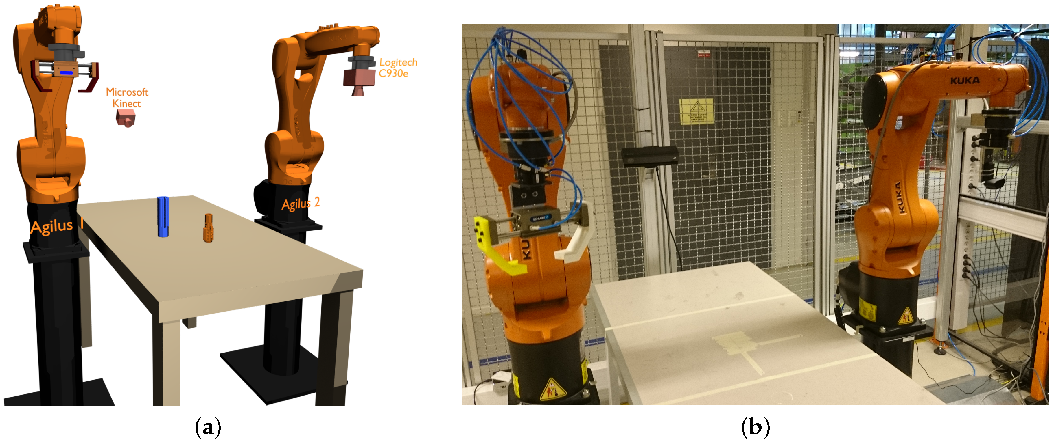
Overview of the robotic cell, where the experiments were conducted. Here, there are two KUKA Agilus robots next to a table. The gripper can be viewed on the robot on the left, while the camera is on the right. Behind the table is the Microsoft Kinect One camera. (a) shows the rendered representation of the cell, while (b) shows the physical cell.
Figure 8.
Overview of the robotic cell, where the experiments were conducted. Here, there are two KUKA Agilus robots next to a table. The gripper can be viewed on the robot on the left, while the camera is on the right. Behind the table is the Microsoft Kinect One camera. (a) shows the rendered representation of the cell, while (b) shows the physical cell.

Figure 9.
The two parts used in all of the experiments. (a) Part A used in the experiment, rendered representation; (b) Part B used in the experiment, rendered representation.
Figure 9.
The two parts used in all of the experiments. (a) Part A used in the experiment, rendered representation; (b) Part B used in the experiment, rendered representation.
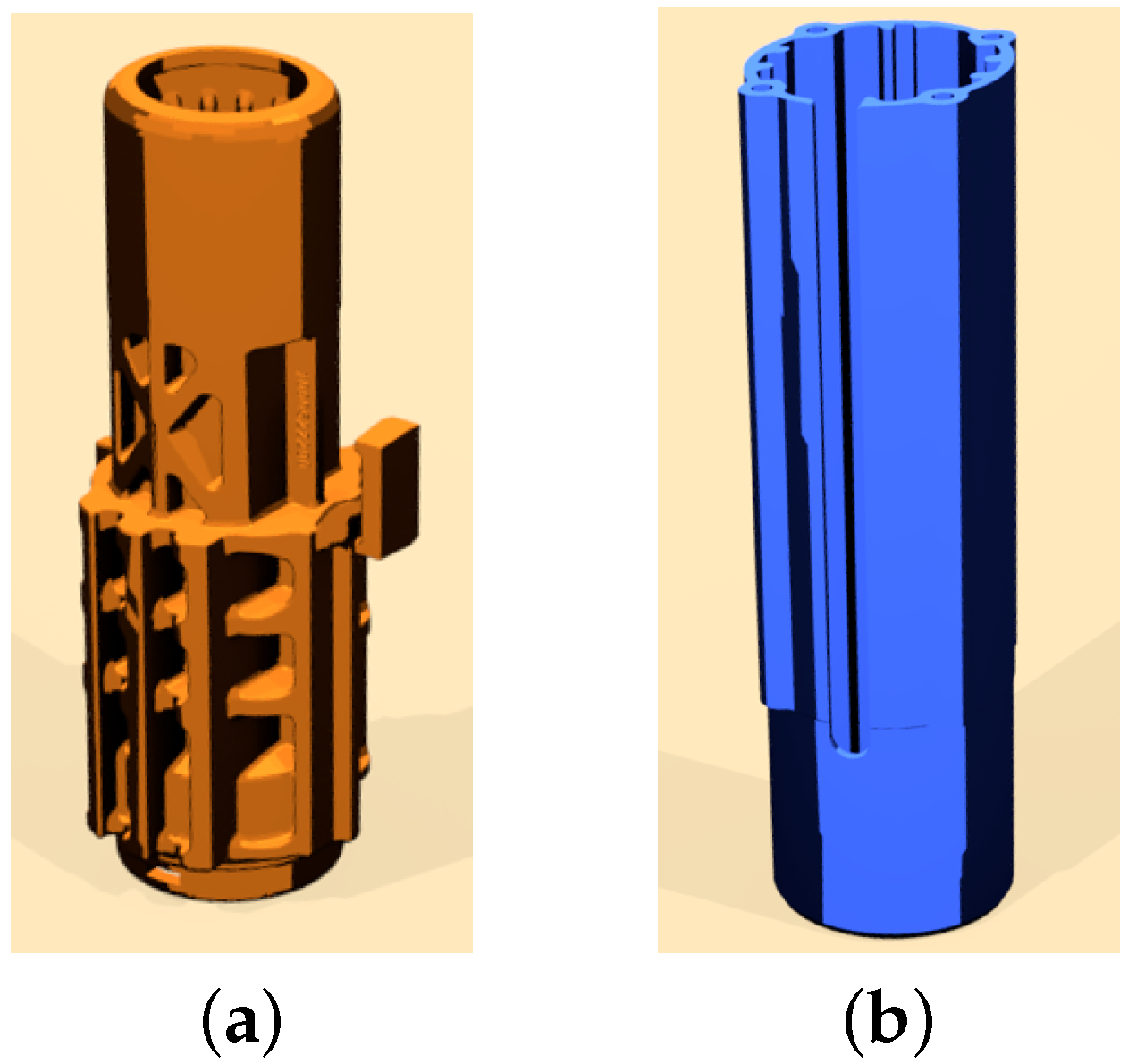
Figure 10.
Top view of the grid and the positioning of the object. Here, nine arbitrary positions of the object is seen. For each of these positions, the rough estimate of the 3D object detection system is calculated.
Figure 10.
Top view of the grid and the positioning of the object. Here, nine arbitrary positions of the object is seen. For each of these positions, the rough estimate of the 3D object detection system is calculated.

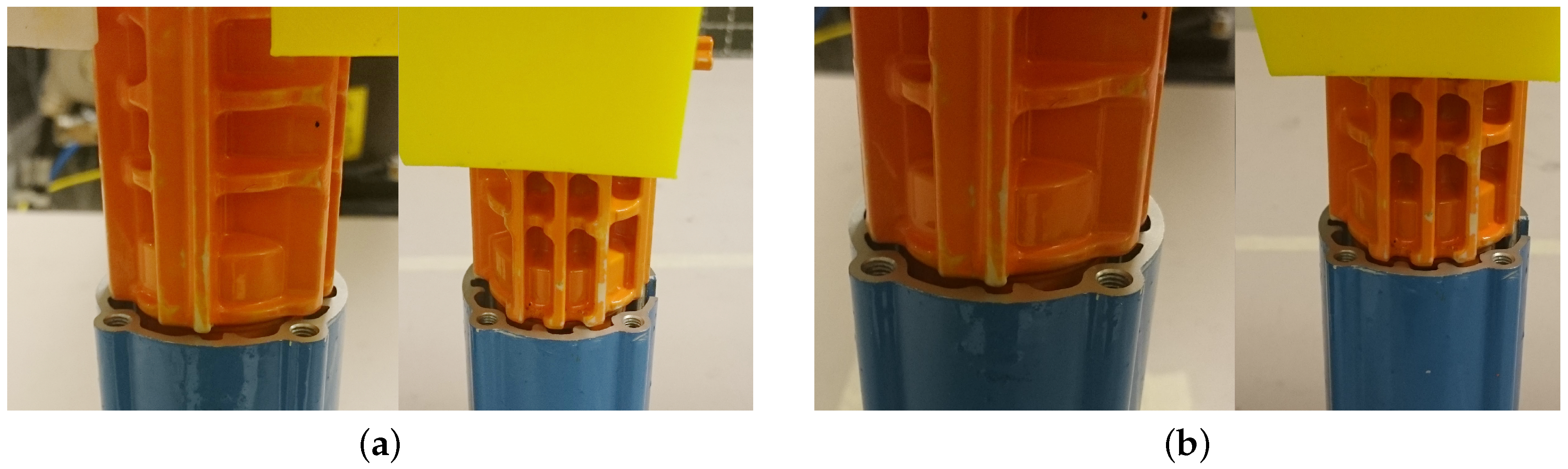
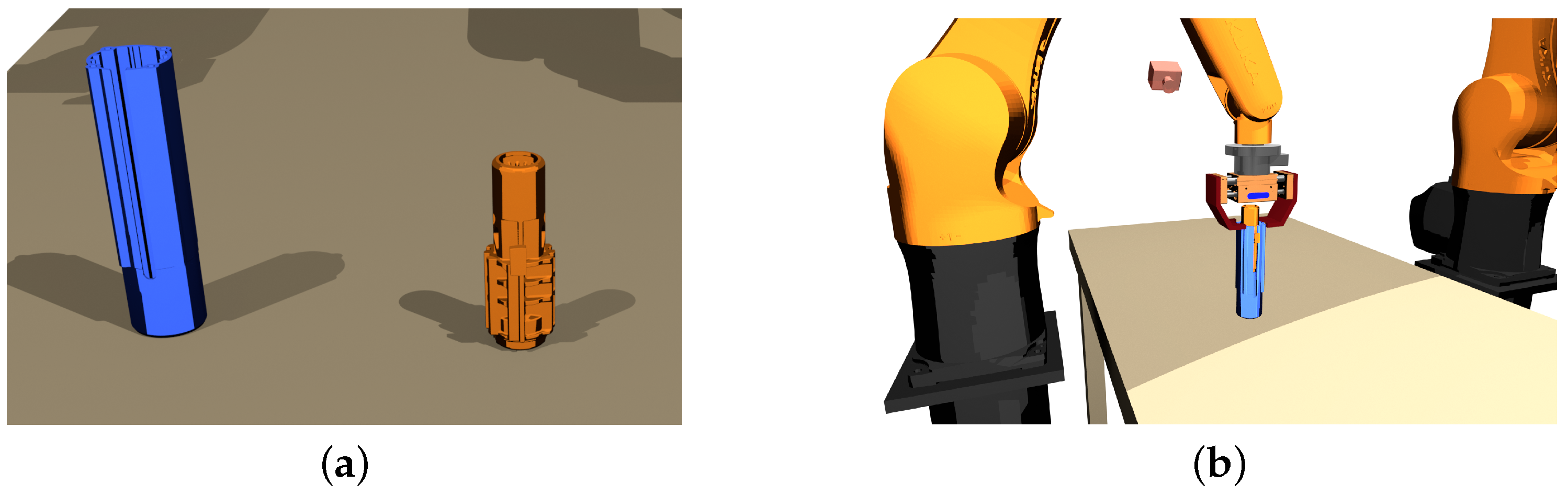
Figure 11.
Overview of the assembly operation. (a) A rendered image of the initial position of the objects; (b) A rendered image of the final position of the objects. It can be seen that the orange object should be assembled inside the blue object.
Figure 11.
Overview of the assembly operation. (a) A rendered image of the initial position of the objects; (b) A rendered image of the final position of the objects. It can be seen that the orange object should be assembled inside the blue object.

Figure 12.
Results from the 3D object detection method. The method successfully classifies each object, and determines a rough estimate of their position.
Figure 12.
Results from the 3D object detection method. The method successfully classifies each object, and determines a rough estimate of their position.

Figure 13.
The small, green circle is the position determined by the 3D object detection. Using this estimate, the method can successfully detect a fine-tuned position using the 2D camera (red circle). The error here is 5.2 mm.
Figure 13.
The small, green circle is the position determined by the 3D object detection. Using this estimate, the method can successfully detect a fine-tuned position using the 2D camera (red circle). The error here is 5.2 mm.
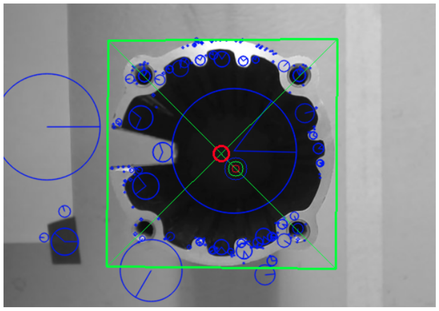
Figure 14.
SIFT used on both objects to determine their position and orientation.
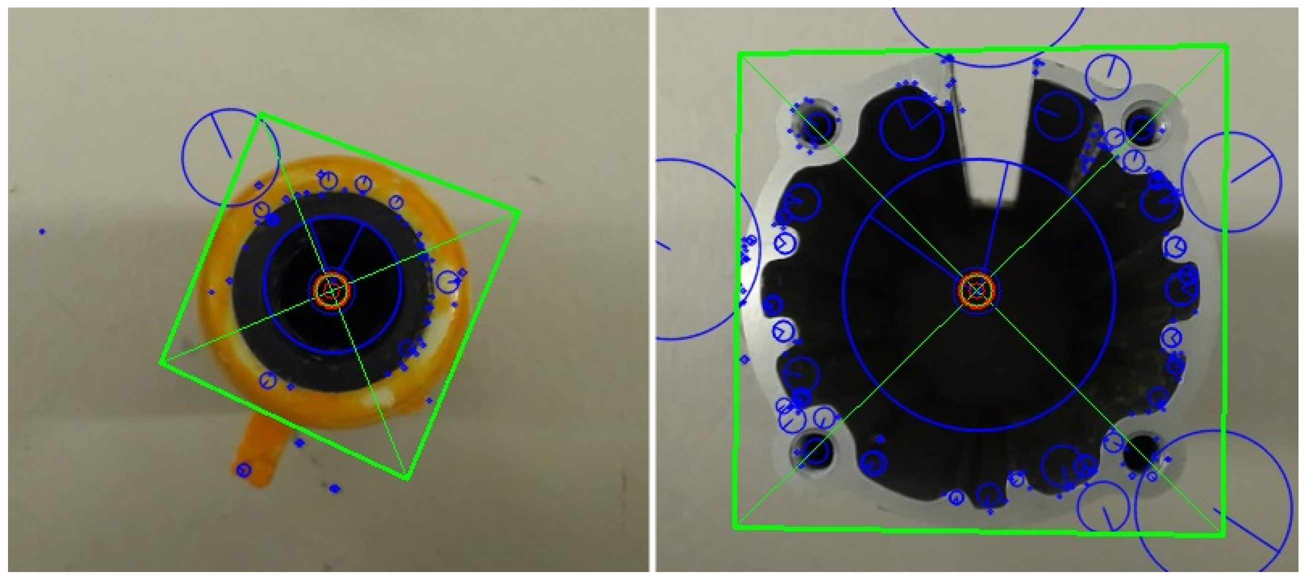
Figure 15.
Depiction of the fail and success conditions. (a) A slight deviation in the angle and position is considered a failure; (b) The position and angle are considered to be correct.
Figure 15.
Depiction of the fail and success conditions. (a) A slight deviation in the angle and position is considered a failure; (b) The position and angle are considered to be correct.

Table 1.
Minimum and maximum deviation between the true position and the estimated position of Object A. The results are based on 25 different estimates.
Table 1.
Minimum and maximum deviation between the true position and the estimated position of Object A. The results are based on 25 different estimates.
| Min/Max Recorded Values | |
|---|---|
| Max [cm] | 1.46 |
| Max [cm] | 1.56 |
| Min [cm] | 0.43 |
| Min [cm] | 0.08 |
Table 2.
Accuracy of detecting Object A (measured in cm). The table shows the true position of Object A, the resulting estimate from the 3D object detection system, and the difference between the two.
Table 2.
Accuracy of detecting Object A (measured in cm). The table shows the true position of Object A, the resulting estimate from the 3D object detection system, and the difference between the two.
| Actual | Measured | Absolute | |||
|---|---|---|---|---|---|
| X | Y | X | Y | ||
| −5 | 5 | −6.18 | 5.4 | 1.18 | 0.4 |
| −5 | 10 | −6.25 | 10.55 | 1.25 | 0.55 |
| −5 | 15 | −6.28 | 16.11 | 1.28 | 1.11 |
| −5 | 20 | −5.17 | 21.56 | 1.28 | 1.56 |
| −10 | 5 | −11.12 | 5.08 | 1.12 | 0.08 |
| −10 | 10 | −10.83 | 10.43 | 0.83 | 0.43 |
| −10 | 15 | −10.98 | 15.92 | 0.98 | 0.92 |
| −10 | 20 | −11.46 | 20.85 | 1.46 | 0.85 |
| −15 | 5 | −15.89 | 5.2 | 0.89 | 0.2 |
| −15 | 10 | −15.81 | 10.56 | 0.81 | 0.56 |
| −15 | 15 | −15.97 | 15.77 | 0.97 | 0.77 |
| −15 | 20 | −16.18 | 21.01 | 1.18 | 1.01 |
| −20 | 5 | −20.43 | 5.4 | 0.43 | 0.4 |
| −20 | 10 | −20.68 | 10.72 | 0.68 | 0.72 |
| −20 | 15 | −20.72 | 16.27 | 0.72 | 1.27 |
| −20 | 20 | −21.18 | 21.38 | 1.18 | 1.38 |
Table 3.
Minimum and maximum deviation between the true position and the estimated position of Object B. The results are based on 25 different estimates.
Table 3.
Minimum and maximum deviation between the true position and the estimated position of Object B. The results are based on 25 different estimates.
| Min/Max Recorded Values | |
|---|---|
| Max [cm] | 1.43 |
| Max [cm] | 1.96 |
| Min [cm] | 0.1 |
| Min [cm] | 0.06 |
Table 4.
Accuracy of detecting Object B (measured in cm). The table shows the true position of Object B, the resulting estimate from the 3D object detection system, and the difference between the two.
Table 4.
Accuracy of detecting Object B (measured in cm). The table shows the true position of Object B, the resulting estimate from the 3D object detection system, and the difference between the two.
| Actual | Measured | Absolute | |||
|---|---|---|---|---|---|
| X | Y | X | Y | ||
| −5 | 5 | −5.76 | 5.16 | 0.76 | 0.16 |
| −5 | 10 | −6.12 | 10.8 | 1.12 | 0.8 |
| −5 | 15 | −5.98 | 15.94 | 0.98 | 0.94 |
| −5 | 20 | −6.17 | 20.88 | 1.17 | 0.88 |
| −10 | 5 | −10.65 | 5.47 | 0.65 | 0.47 |
| −10 | 10 | −10.62 | 10.21 | 0.62 | 0.21 |
| −10 | 15 | −10.73 | 15.81 | 0.73 | 0.81 |
| −10 | 20 | −10.91 | 20.79 | 0.91 | 0.79 |
| −15 | 5 | −15.22 | 5.46 | 0.22 | 0.46 |
| −15 | 10 | −15.46 | 10.62 | 0.46 | 0.62 |
| −15 | 15 | −15.71 | 16.2 | 0.71 | 1.2 |
| −15 | 20 | −15.85 | 21.14 | 0.85 | 1.14 |
| −20 | 5 | −20.1 | 5.43 | 0.1 | 0.43 |
| −20 | 10 | −20.73 | 10.06 | 0.73 | 0.06 |
| −20 | 15 | −20.26 | 16.35 | 0.26 | 1.35 |
| −20 | 20 | −21.43 | 21.96 | 1.43 | 1.96 |
Table 5.
The difference between the maximum and minimum measured orientations for Object A. The first table is the deviation between the maximum and minimum angle when the object is positioned at 0°, both with using SIFT and with a SIFT/SURF hybrid. The second table is when the object is positioned at 90°. The measurements are given in degrees.
| 0 Degrees | −90 Degrees | ||
|---|---|---|---|
| SIFT | SIFT/SURF | SIFT | SIFT/SURF |
| 1.7469 | 5.4994 | 1.1102 | 7.9095 |
Table 6.
The difference between the maximum and minimum measured orientations for Object B. The first table is the deviation between the maximum and minimum angle when the object is positioned at 0°, both with using SIFT, and with a SIFT/SURF hybrid. The second table is when the object is positioned at 90°. The measurements are given in degrees.
| 0 Ddegree | −90 Degrees | ||
|---|---|---|---|
| SIFT | SURF | SIFT | SURF |
| 0.07888 | 0.2041 | 0.1721 | 0.1379 |
© 2017 by the authors. Licensee MDPI, Basel, Switzerland. This article is an open access article distributed under the terms and conditions of the Creative Commons Attribution (CC BY) license (http://creativecommons.org/licenses/by/4.0/).
Share and Cite
MDPI and ACS Style
Kleppe, A.L.; Bjørkedal, A.; Larsen, K.; Egeland, O. Automated Assembly Using 3D and 2D Cameras. Robotics 2017, 6, 14. https://doi.org/10.3390/robotics6030014
AMA Style
Kleppe AL, Bjørkedal A, Larsen K, Egeland O. Automated Assembly Using 3D and 2D Cameras. Robotics. 2017; 6(3):14. https://doi.org/10.3390/robotics6030014
Chicago/Turabian StyleKleppe, Adam Leon, Asgeir Bjørkedal, Kristoffer Larsen, and Olav Egeland. 2017. "Automated Assembly Using 3D and 2D Cameras" Robotics 6, no. 3: 14. https://doi.org/10.3390/robotics6030014
Note that from the first issue of 2016, this journal uses article numbers instead of page numbers. See further details here.