Compressed Voxel-Based Mapping Using Unsupervised Learning
by
 , and
, and
Daniel Ricao Canelhas
1,* ,
,
Erik Schaffernicht
1,
Todor Stoyanov
1,
Achim J. Lilienthal
1 and
Andrew J. Davison
2 1
Center of Applied Autonomous Sensor Systems (AASS), Örebro University, Örebro 701 82, Sweden
2
Department of Computing, Imperial College London, London SW7 2AZ, UK
*
Author to whom correspondence should be addressed.
Robotics 2017, 6(3), 15; https://doi.org/10.3390/robotics6030015
Submission received: 11 May 2017
/
Revised: 20 June 2017
/
Accepted: 26 June 2017
/
Published: 29 June 2017
(This article belongs to the Special Issue Robotics and 3D Vision)
Abstract
:In order to deal with the scaling problem of volumetric map representations, we propose spatially local methods for high-ratio compression of 3D maps, represented as truncated signed distance fields. We show that these compressed maps can be used as meaningful descriptors for selective decompression in scenarios relevant to robotic applications. As compression methods, we compare using PCA-derived low-dimensional bases to nonlinear auto-encoder networks. Selecting two application-oriented performance metrics, we evaluate the impact of different compression rates on reconstruction fidelity as well as to the task of map-aided ego-motion estimation. It is demonstrated that lossily reconstructed distance fields used as cost functions for ego-motion estimation can outperform the original maps in challenging scenarios from standard RGB-D (color plus depth) data sets due to the rejection of high-frequency noise content.
1. Introduction
A signed distance field (SDF), sometimes referred to as a distance function, is an implicit surface representation that embeds geometry into a scalar field whose defining property is that its value represents the distance to the nearest surface of the embedded geometry. Additionally, the field is positive outside the geometry, i.e., in free space, and negative inside. SDFs have been extensively applied to e.g., speeding up image-alignment [1] and raycasting [2] operations as well as collision detection [3], motion planning [4] and articulated-body motion tracking [5]. The truncated SDF [6] (TSDF), which is the focus of the present work, side-steps some of the difficulties that arise when fields are computed and updated based on incomplete information. This has proved useful in applications of particular relevance to the field of robotics research: accurate scene reconstruction ([7,8,9]) as well as for rigid-body ([10,11]) pose estimation.
The demonstrated practicality of distance fields and other voxel-based representations such as occupancy grids [12] and the direct applicability of a vast arsenal of image processing methods to such representations make them a compelling research topic. However, a major drawback in such representations is the large memory requirement for storage, which severely limits their applicability for large-scale environments. For example, a space measuring m mapped with voxels of 2 cm size requires at least 800 MB at 32 bits per voxel.
Mitigating strategies, such as cyclic buffers ([8,9]), octrees ([13,14]), and key-block swapping [15], have been proposed to limit the memory cost of using volumetric distance-fields in very different ways. In the present work, we address the issue of volumetric voxel-based map compression by an alternative strategy. We propose encoding (and subsequently decoding) the TSDF in a low-dimensional feature space by projection onto a learned set of basis (eigen-) vectors derived via principal component analysis [16] (PCA) of a large data set of sample reconstructions. We also show that this compression method preserves important structures in the data while filtering out noise, allowing for more stable camera-tracking to be done against the model, using the SDF Tracker [10] algorithm. We show that this method compares favorably to nonlinear methods based on auto-encoders (AE) in terms of compression, but slightly less so in terms of tracking performance.
The proposed compression strategies can be applied to scenarios in which robotic agents with limited on-board memory and computational resources need to map large spaces. The actively reconstructed TSDF need only be a small fraction of the size of the entire environment and be allowed to move. The regions that are no longer observed can be efficiently compressed into a low-dimensional feature space and re-observed regions can be decompressed back into the original TSDF representation. Although the compression is lossy, most of the content is lost in the higher-frequency domain which we show to have positive side effects in terms of noise removal. When a robot re-observes previously explored regions of a compressed map, the low-dimensional feature representation may serve as a descriptor, providing an opportunity for the robot to, still in the descriptor-space, make the decision to selectively decompress regions of the map that may be of particular interest. A proof of concept for this scenario and tracking performance evaluations on lossily reconstructed maps are presented in Section 5.
The remainder of the paper is organized as follows: an overview on related work in given in Section 2. In Section 3, we formalize the definition of TSDFs, and present a brief introduction to the topics of PCA and AE networks. In Section 4, we elaborate on the training data used, followed by a description of our evaluation methodology. Section 5 contains experimental results, followed by Section 7, which presents some possible extensions to the present work, and Section 6 lastly presents our conclusions.
2. Related Work
Our work is perhaps most closely related to sparse coded surface models [17] which use K-SVD [18] to reduce the dimensionality of textured surface patches. K-SVD is an algorithm that generalizes k-means clustering to learn a sparse dictionary of code words that can be linearly combined to reconstruct data. Another recent contribution in this category is the Active Patch Model for 2D images [19]. Active patches consist of a dictionary of data patches in input space that can be warped to fit new data. A low-dimensional representation is derived by optimizing the selection of patches and pre-defined warps that best use the patches to reconstruct the input. The operation on surface patches instead of volumetric image data is more efficient for compression for smooth surfaces, but may require an unbounded number of patches for arbitrarily complex geometry. As an analogy, our work can be thought of as an application of eigenfaces [20] to the problem of 3D shape compression and low-level scene understanding. Operating directly on a volumetric representation, as we propose, has the advantage of a constant compression ratio per unit volume, regardless of the surface complexity, as well as avoiding the problem of estimating the optimal placement of patches. The direct compression of the TSDF also permits the proposed method to be integrated into several popular algorithms that rely on this representation, with minimal overhead. There are a number of data-compression algorithms designed for directly compressing volumetric data. Among these, we find video and volumetric image compression ([21,22]), including work dealing with distance fields specifically [23]. Although these methods produce high-quality compression results, they typically require many sequential operations and complex extrapolation and/or interpolation schemes. A side effect of this is that these compressed representations may require information far from the location that is to be decoded. They also do not generate a mapping to a feature space wherein similar inputs map to similar features, so possible uses as descriptors are limited at best.
3. Preliminaries
3.1. Truncated Signed Distance Fields (TSDF)
TSDFs are three-dimensional image structures that implicitly represent geometry by sampling, typically on a uniform lattice, the distance to the nearest surface. A sign is used to indicate whether the distance is sampled from within a solid shape (negative, by convention) or in free space (positive). The approximate location of surfaces can be extracted as the zero level set. Let
be defined as the distance field of some arbitrary closed surface in in ,
Given the closed (no holes) property of the surface, one may assume that every surface point has an associated outward-oriented normal vector (). The expression then consistently attributes a sign to indicate on which side of the surface is located. Finally, truncating the value of the field in an interval produces the TSDF,
defined, for any closed surface, as
3.2. Principal Component Analysis (PCA)
PCA [16] is a method for obtaining a linear transformation into a new orthogonal coordinate system. In this system, the first dimension is associated with the direction, in a data set, that exhibits the largest variance. The second dimension is aligned with a direction, perpendicular to the first, along which the second most variance is exhibited and so on. We achieve this by first subtracting the data set mean from each sample in the data matrix (centering) and then applying a singular value decomposition (SVD). SVD creates a principal component matrix of elements, producing a mapping from input space into a new space of orthogonal basis vectors, one for each singular value. The magnitude of these singular values relate to the amount of variance observed along their associated basis vector in the data set and can be sorted in descending order, the smallest of which are typically close to zero. This suggests that some columns from the principal component matrix can be removed, as they are related to the lower-variance components.
Multiplying a (centered) vector from the input space, i.e., a voxel block unrolled into a vector (of 4096 elements), with the reduced set of principal components then projects the voxel data onto a lower-dimensional space. Inversely, multiplying a lower-dimensional vector from the feature space with the transpose of the principal component matrix, maps back into the input space. The resulting voxel block is then a low-rank approximation of the initial data.
Writing the singular value decomposition of our centered data-matrix as
The matrix contain the principal components of the data. For any given sample, in input space, we can generate a descriptor of lower dimensionality:
Mapping back to the input space is done by computing,
Using PCA, we can thus design low-dimensional descriptors for the high-dimensional voxel chunks, while making use of statistics related to the training data set to pick a good approximation.
3.3. Artificial Neural Network
Artificial neural networks (ANNs) are often described using biological analogies, as a nonlinear computational architecture with several layers that connect multiple inputs to outputs as the weighted sum of their contributions, plus some bias. For a fully connected neural network, this is essentially a vector-matrix product followed by addition. Described is an affine function that could be replaced by a single layer of multiplication without any loss. However, nonlinear properties are introduced by applying an element-wise activation function on the vector resulting from the computation at each layer. A descriptor can thus be computed from the input vector p by chaining the multiplications with layers through interleaved with element-wise activation functions f,
Finding an appropriate set of weights for the layers and biases is done by comparing the output of the network with some reference and minimizing an objective related to this error using numerical optimization techniques. This optimization process is appropriately called “training” the network.
Training an ANN as an auto-encoder can be done in a straightforward manner by setting its desired output to be equal to its input and employing e.g., back-propagation [24] to minimize the difference over a large quantity of representative data from the target domain. For some form of encoding to occur, it is required that somewhere in between the input layer and output layer, there exists an intermediary hidden layer whose dimensionality is smaller than those of the input and output (which are the of the same size). We refer to this intermediate “bottleneck” layer as a code or feature layer. The portion of the ANN up until the feature layer can then be treated as an encoder and the portion after is treated as a decoder. For practical reasons (particularly when layer-wise unsupervised pre-training is involved [25]), it makes sense to keep the encoder and decoder symmetric.
4. Methodology
4.1. Training Data
The data set used for training consists of sub-volumes sampled from 3D reconstructions of real-world industrial and office environments c.f. Figure 1. These reconstructions are obtained by fusing sequences of depth images into a TSDF as described in [6] with truncation limits set to and . Camera pose estimates were produced by the SDF Tracker algorithm (though any method with low drift would do just as well). The real-world data are augmented by synthetic samples of TSDFs, procedurally generated using libsdf [26], an open-source C++ library that implements simple implicit geometric primitives (as described in [2,27]). Some examples from our synthetic data set can be seen in Figure 2.
Sub-volumes were sampled from the real-world reconstructions by taking samples at every eight voxels along each spatial dimension and permuting the indexing order along each axis for every sample to generate five additional reflections at each location. Distance values are then mapped from the interval to and saved. Furthermore, to avoid a disproportionate amount of samples of empty space, sub-volumes for which the mean sum of normalized () distances is below are discarded, and a small proportion of empty samples is explicitly included instead.
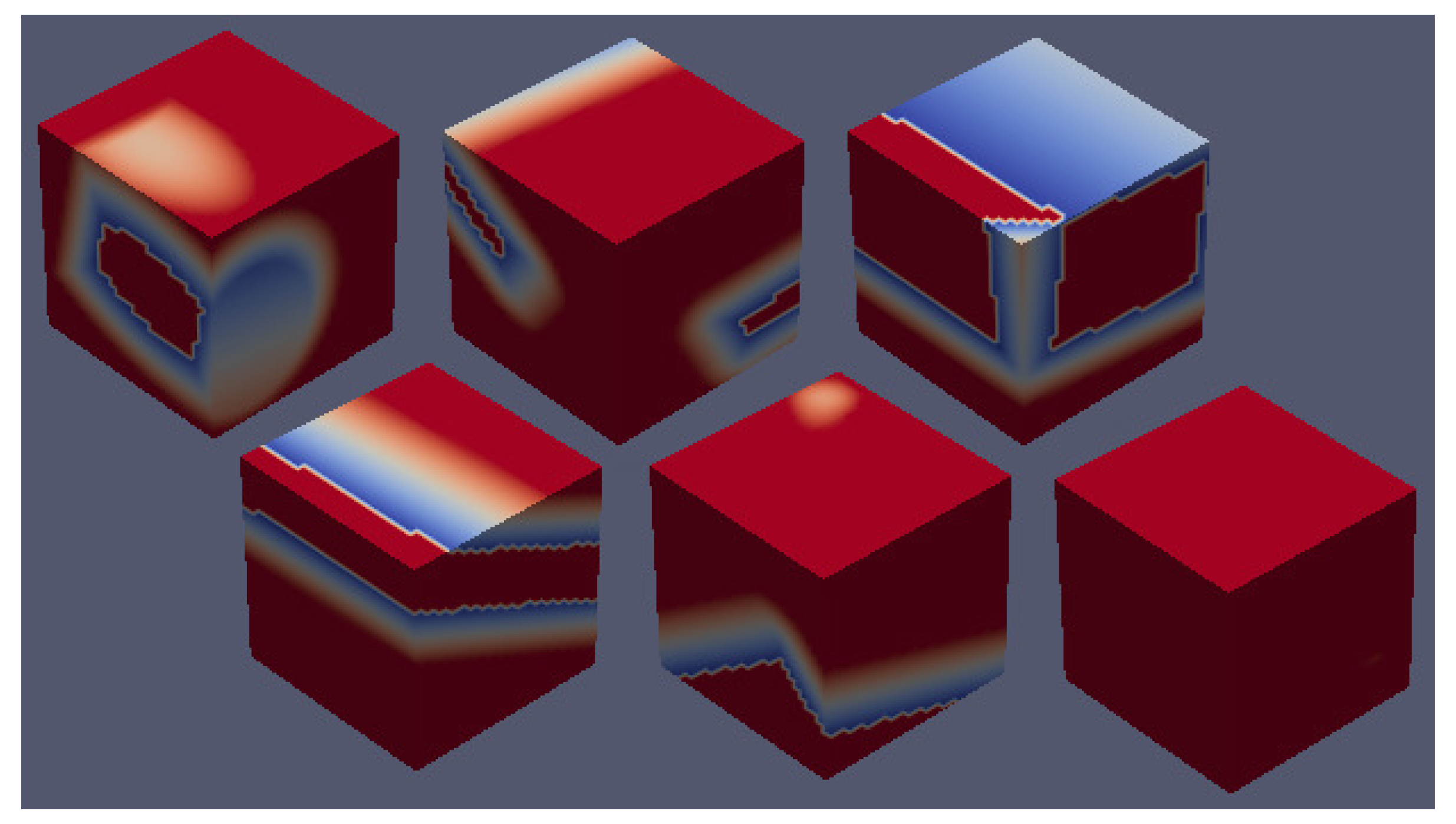
The procedurally generated shapes were sampled in the same manner as the real-world data. It was generated by randomly picking a sequence of randomly parametrized and oriented shapes from several shape categories representing fragments of: flat surfaces, concave edges, convex edges, concave corners, convex corners, rounded surfaces, and rounded edges. For non-oriented surfaces, convexity and concavity does not matter, since one is representable by a rotation of the other, but need to be represented as separate cases here, since the sign is inverted in the TSDF. The distances are truncated and converted to the same intervals as with the real data. The use of synthetic data allows generating training examples in a vast number of poses, with a greater degree of geometric variation than would be feasible to collect manually through scene reconstructions alone.
The sub-volumes, when unrolled, define an input of a dimensionality equal to (i.e., ), and the combined number of samples number . Our data set is then .
4.2. Evaluation Methodology
Having defined methods for obtaining features, either using PCA or ANN, what is a good balance between compression ratio and map quality in the context of robotics? We explore this question by means of two different fitness quality measures. Reconstruction fidelity and ego-motion estimation. To aid in our analysis, we use a publicly available RGB-D (color plus depth) data set [28] with ground truth pose estimates provided by an independent external camera-tracking system. Using the provided ground truth poses, we generate a map, by fusing the depth images into a TSDF representation. This produces a ground truth map. We chose teddy, room, desk, desk2, 360 and plant from the freiburg-1 collection for evaluation as these are representative of real-world challenges that arise in simultaneous localization and mapping (SLAM) and visual odometry, including motion blur, sensor noise and occasional lack of geometric structure needed for tracking. We do not use the RGB components of the data for any purpose in this work. We perform two types of experiments, designed to test the reconstruction fidelity and the reliability of tracking algorithms operating on the reconstructed volume.
As a measure for reconstruction error, we compute the mean squared errors of the decoded distance fields relative to the input. This metric is relevant to path planning, manipulation and object detection tasks since it indirectly relates to the fidelity of surface locations. For each data set, using each encoder/decoder, we compute a lossy version of the original data and report the average and standard deviation across all data sets.
Ego-motion estimation performance is measured by the absolute trajectory error (ATE) [28]. The absolute trajectory error is the integrated distance between all pose estimates relative to the ground truth trajectory. The evaluations are performed by loading a complete TSDF map into memory and setting the initial pose according to ground truth. Then, as depth images are loaded from the RGB-D data set, we estimate the camera transformation that minimizes the point to model distance for each new frame. The evaluation was performed on all the data sets, processed through each compression and subsequent decompression method. As a baseline, we also included the original map, processed with a Gaussian blur kernel of size 9 × 9 × 9 voxels and a parameter of .
Building on the experimental results, we are able to demonstrate two applications: selective map decompression based on descriptor matching and large-scale mapping in a dense TSDF space, by fast on-the-fly compression and decompression.
5. Experimental Results
The PCA basis was produced, using the dimensionality reduction tools from the scikit-learn [29] library. Autoencoders were trained using pylearn2 [30] using batch gradient descent with the change in reconstruction error on a validation data set as a stopping criterion. The data set was split into 400 batches containing 500 samples each, of which 300 batches were used for training, 50 for testing, and 50 for validation. The networks use sigmoid activation units and contain nodes, with d representing the number of dimensions of the descriptor.
The runtime implementation for the encoder/decoder architectures was done using the cuBLAS [31] and Thrust [32] libraries, enabling matrix-vector and array computation on the graphics processing unit (GPU).
5.1. Reconstruction Error
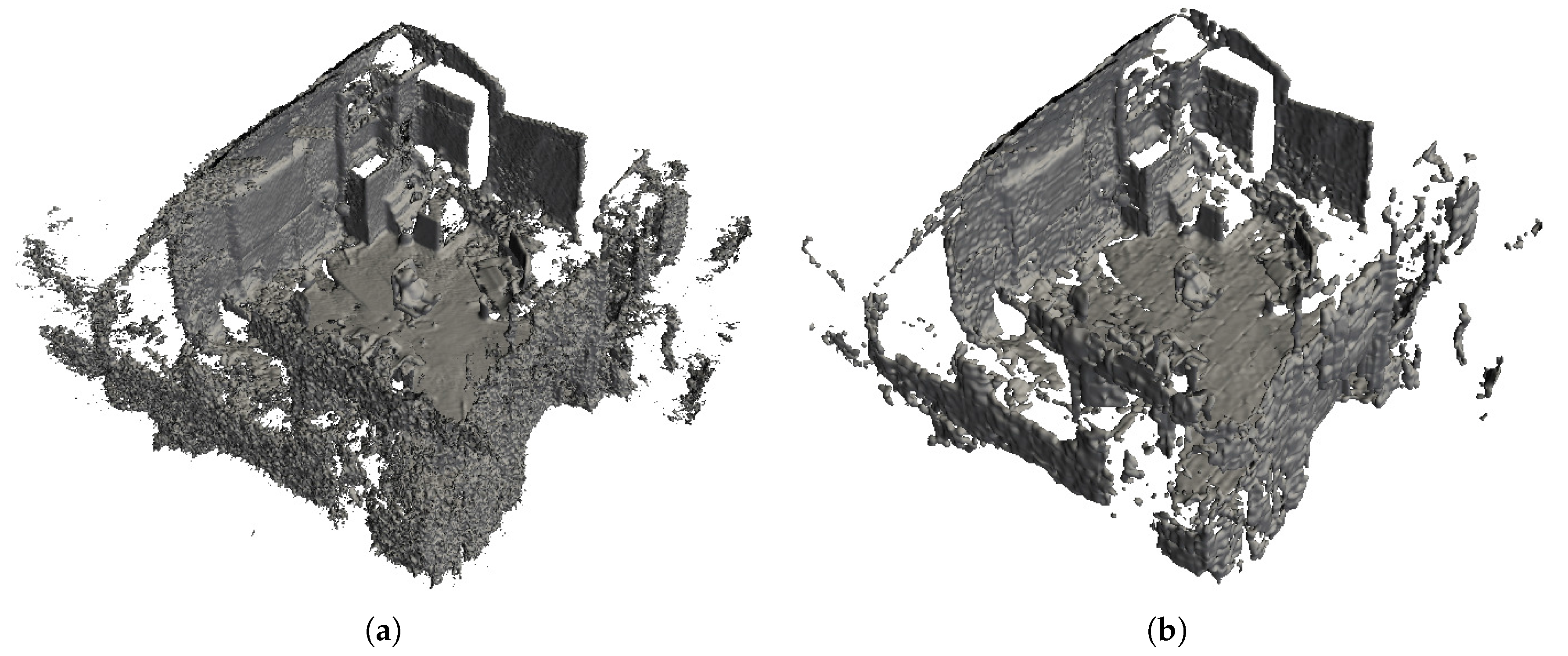
We report the average reconstruction error over all non-empty blocks in all data sets and the standard deviation among data sets in Table 1. The reconstruction errors obtained strongly suggest that increasing the size of the codes for individual encoders yields better performance, though with diminishing returns. Several attempts were made, to out-perform the PCA approach, using Artificial Neural Networks (ANN) trained as auto-encoders, but this was generally unsuccessful. PCA-based encoders, using 32, 64 and 128 components, produce better results than ANN encoders in all of our experiments.
The best overall reconstruction performance is given by the PCA encoder/decoder, using 128 components. We illustrate this with an image from the teddy data set in Figure 3. Note that the decoded data set is smoother, so, in a sense, the measured discrepancy is partly related to a qualitative improvement.
5.2. Ego-Motion Estimation
The ego-motion estimation, performed by the SDF Tracker algorithm, uses the TSDF as a cost function to which subsequent 3D points are aligned. This requires that the gradient of the TSDF be of correct magnitude and point in the right direction. To get a good alignment, the minimum absolute distance should coincide with the actual location of the surface.
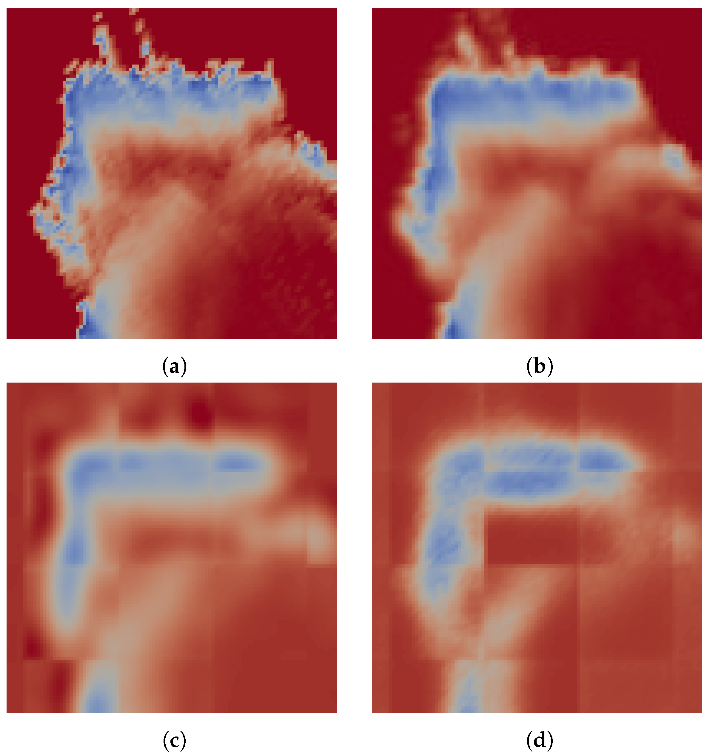
In spite of being given challenging camera trajectories, performance using the decoded maps is on average better than the unaltered map. When the tracker keeps up with the camera motion, we have observed that the performance resulting from the use of each map is in the order of their respective reconstruction errors. In this case, the closer the surface is to the ground truth model, the better. However, tracking may fail for various reasons, e.g., when there is little overlap between successive frames, when the model or depth image contains noise or when there is not enough geometric variation to properly constrain the pose estimation. In some of these cases, the maps that offer simplified approximations to the original distance field fare better. The robustness in tracking is most likely owed to the denoising effect that the encoding has, as evidenced by the performance on the Gaussian blurred map. Of the encoded maps, we see that the AE compression results in better pose estimation. In Figure 4, we see a slice through a volume color-coded by distance. Here, we note that, even though the PCA-based map is more similar to the original, on the left side of the image, it is evident that the field is not monotonically increasing away from the surface. Such artifacts cause the field gradient to point in the wrong direction, possibly contributing to failure in finding the correct alignment. The large difference between the median and mean values for the pose estimation errors are indicative of mostly accurate pose estimations, with occasional gross misalignments.
5.3. Selective Feature-Based Map Expansion
Although the descriptors we obtain are clearly not invariant to affine transformations (if they were, the decompression would not reproduce the field in its correct location/orientation), we can still create descriptor-based models for geometries of particular interest by sampling their TSDFs over the range of transformations to which we want the model to be invariant. If information about the orientation of the map is known a priori, e.g., some dominant structures are axis-aligned with the voxel lattice, or dominant structures are orthogonal to each other, the models can be made even smaller. In the example illustrated in Figure 5, a descriptor-based model for floors was first created by encoding the TSDFs of horizontal planes at 15 different offsets, generating one 64-element vector each. Each descriptor in the compressed map can then be compared to this small model by the squared norm of their differences and only those beneath a threshold of similarity need to be considered for expansion. Here, an advantage of the PCA-based encoding becomes evident: since PCA generates its linear subspace in an ordered manner, feature vectors of different dimensionality can be tested for similarity up to the number of elements of the smallest, i.e., a 32-dimensional feature descriptor can be matched against the first half of a 64-dimensional feature descriptor. This property is useful in handling multiple levels of compression, for different applications, whilst maintaining a common way to describe them.
5.4. Large-Scale Mapping
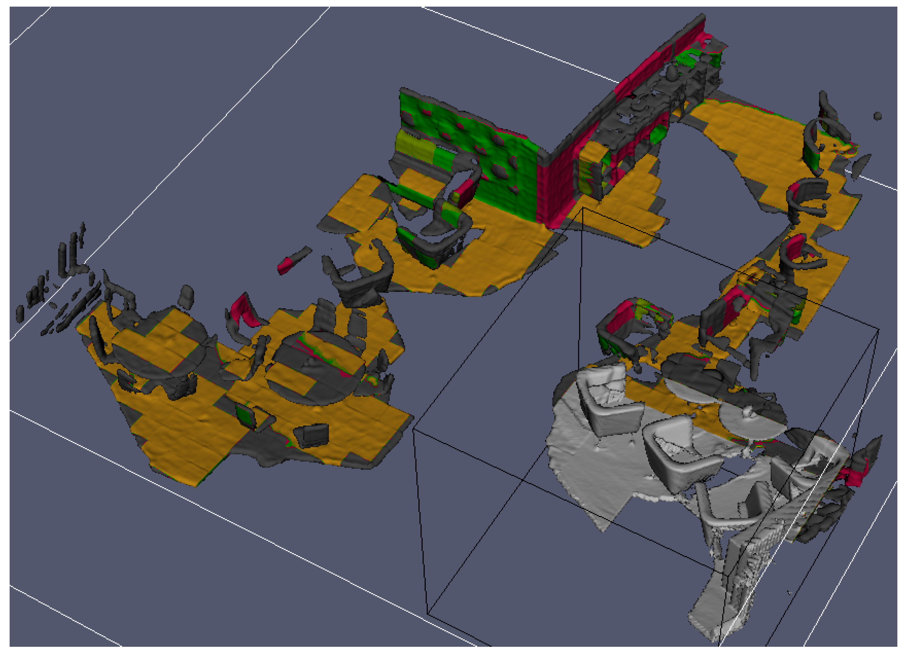
By extending the SDF Tracker algorithm with a moving active volume centered around the camera translation vector, for every 16-voxel increment, we can encode the voxel blocks exiting the active TSDF on the lagging end, (if not empty), and decode the voxel blocks entering the active TSDF on the front end (if they contain a previously stored descriptor). This allows mapping much larger areas, since each voxel block can be reduced from its 4096 voxels to the chosen size of a descriptor or a token, if the block is empty. Since the actual descriptor computation happens on the GPU, the performance impact on the tracking and mapping part of the algorithm is not too severe. An example of this is shown in Figure 6.
The tracking and mapping algorithm itself is a real-time capable system with performance that scales with the size of the volume and resolution of the depth images given as input. While it only handles volumes of approximately voxels at QVGA resolution (320 × 240 pixels) and lower at 30 Hz, it does so solely on an Intel i7-4770K 3.50 GHz CPU (Örebro, Sweden). This leaves the GPU free to perform on-the-fly compression and decompression.
Timing the execution of copying data to the GPU, encoding, decoding and copying it back to the main CPU memory results in an average between 405 and 520 s per block of voxels on a Nvidia GTX Titan GPU (Örebro, Sweden). For an active TSDF volume of 160 × 160 × 160 voxels, shifting one voxel-block sideways would result in 100 blocks needing to be encoded, 100 blocks decoded, and memory in both directions’ transfers, in the worst case. Our round-trip execution timing puts this operation at approximately 41 to 52 milliseconds.
The span in timings depend on the encoding method used, with PCA-based encoding representing the lower end and ANN the upper, for descriptors of 128 elements.
6. Conclusions
In this paper, we presented the use of dimensionality reduction of TSDF volumes, which lie at the core of many algorithms across a wide domain of applications with close ties to robotics. We proposed PCA and ANN encoding strategies and evaluated their performance with respect to a camera tracking application and to reconstruction error.
We demonstrate that we can compress volumetric data using PCA and neural nets to small sizes (between 128:1 and 32:1) and still use them in camera tracking applications with good results. We show that PCA produces superior reconstruction results and although neural nets have inherently greater expressive power, training them is not straightforward, often resulting in lower quality reconstructions but nonetheless offering slightly better performance in ego-motion estimation applications. Finally, we have shown that this entire class of methods can be successfully applied to both compress and imbue the data with some low-level semantic meaning and suggested an application in which both of these characteristics are simultaneously desirable.
7. Future Work
It is clear that the resulting features are not invariant to rigid-body transformations and experimentally matching features of identical objects in different poses suggests that features do not form object-centered clusters in the lower-dimensional space. A method for obtaining a low-dimensional representation as well as a reliable transformation into some canonical frame of reference would pave the way for many interesting applications in semantic mapping and scene understanding. Furthermore, it seems unfortunate that pose-estimation ultimately has to occur in the voxel domain. Given that the transformation to the low-dimensional space is a simple affine function (at least for the PCA-based encoding), it seems intuitive that one should be able to formulate and solve the pose-estimation problem in the reduced space with a lower memory requirement in all stages of computation. Investigating this possibility remains an interesting problem, as it is not clear if this would represent a direct trade-off between memory complexity and computational complexity.
Acknowledgments
This work has partly been supported by the European Commission under contract number FP7-ICT-270350 (RobLog) and within H2020-ICT under grant agreement number 732737 (ILIAD).
Author Contributions
Conception of the work: Daniel Ricao Canelhas, Erik Schaffernicht, Todor Stoyanov, Andrew J. Davison; Data collection: Daniel Ricao Canelhas; Data analysis and interpretation: Daniel Ricao Canelhas, Erik Schaffernicht, Todor Stoyanov; Drafting the article: Daniel Ricao Canelhas; Critical revision of the article: Erik Schaffernicht, Todor Stoyanov, Achim J. Lilienthal, Andrew J. Davison; Final approval of the version to be published: Daniel Ricao Canelhas, Erik Schaffernicht, Todor Stoyanov, Achim J. Lilienthal, Andrew J. Davison.
Conflicts of Interest
The authors declare no conflict of interest.
References
- Fitzgibbon, A.W. Robust Registration of 2D and 3D Point Sets. Image Vis. Comput. 2003, 21, 1145–1153. [Google Scholar] [CrossRef]
- Hart, J.C. Sphere tracing: A geometric method for the antialiased ray tracing of implicit surfaces. Vis. Comput. 1996, 12, 527–545. [Google Scholar] [CrossRef]
- Fuhrmann, A.; Sobotka, G.; Groß, C. Distance fields for rapid collision detection in physically based modeling. In Proceedings of the 2003 International Conference Graphicon, Moscow, Russia, 5–10 September 2003; pp. 58–65. [Google Scholar]
- Hoff, K.E., III; Keyser, J.; Lin, M.; Manocha, D.; Culver, T. Fast computation of generalized voronoi diagrams using graphics hardware. In Proceedings of the 26th Annual Conference on Computer Graphics and Interactive Techniques, Los Angeles, CA, USA, 8–13 August 1999; ACM Press/Addison-Wesley Publishing Co.: New York, NY, USA, 1999; pp. 277–286. [Google Scholar]
- Schmidt, T.; Newcombe, R.; Fox, D. DART: Dense articulated real-time tracking. In Proceedings of the Robotics: Science and Systems, Berkeley, CA, USA, 12–16 July 2014; ISBN 978-0-9923747-0-9. [Google Scholar]
- Curless, B.; Levoy, M. A volumetric method for building complex models from range images. In Proceedings of the 23rd Annual Conference on Computer Graphics and Interactive Techniques, New Orleans, LA, USA, 4–9 August 1996; ACM: New York, NY, USA, 1996; pp. 303–312. [Google Scholar]
- Newcombe, R.A.; Davison, A.J.; Izadi, S.; Kohli, P.; Hilliges, O.; Shotton, J.; Molyneaux, D.; Hodges, S.; Kim, D.; Fitzgibbon, A. KinectFusion: Real-time dense surface mapping and tracking. In Proceedings of the 2011 10th IEEE International Symposium on Mixed and Augmented Reality (ISMAR), Basel, Switzerland, 26–29 October 2011; pp. 127–136. [Google Scholar]
- Whelan, T.; Kaess, M.; Fallon, M.; Johannsson, H.; Leonard, J.; McDonald, J. Kintinuous: Spatially extended KinectFusion. In Proceedings of the RSS Workshop on RGB-D: Advanced Reasoning with Depth Cameras, Sydney, Australia, 9–13 July 2012. [Google Scholar]
- Roth, H.; Vona, M. Moving volume kinectfusion. In Proceedings of the British Machine Vision Conference (BMVC) 2012, Surrey, UK, 3–7 September 2012; pp. 1–11. [Google Scholar]
- Canelhas, D.R.; Stoyanov, T.; Lilienthal, A.J. Sdf tracker: A parallel algorithm for on-line pose estimation and scene reconstruction from depth images. In Proceedings of the 2013 IEEE/RSJ International Conference on Intelligent Robots and Systems (IROS), Tokyo, Japan, 3–7 November 2013; pp. 3671–3676. [Google Scholar]
- Bylow, E.; Sturm, J.; Kerl, C.; Kahl, F.; Cremers, D. Real-time camera tracking and 3d reconstruction using signed distance functions. In Proceedings of the Robotics: Science and Systems, Berlin, Germany, 24–28 June 2013. [Google Scholar]
- Elfes, A. Occupancy Grids: A Probabilistic Framework for Robot Perception and Navigation. Ph.D. Thesis, Carnegie Mellon University, Pittsburgh, PA, USA, 1989. [Google Scholar]
- Frisken, S.F.; Perry, R.N.; Rockwood, A.P.; Jones, T.R. Adaptively sampled distance fields: A general representation of shape for computer graphics. In Proceedings of the 27th Annual Conference on Computer Graphics and Interactive Techniques, New Orleans, LA, USA, 23–28 July 2000; ACM Press/Addison-Wesley Publishing Co.: New York, NY, USA, 2000; pp. 249–254. [Google Scholar]
- Zeng, M.; Zhao, F.; Zheng, J.; Liu, X. A memory-efficient kinectfusion using octree. In Computational Visual Media; Springer: New York, NY, USA, 2012; pp. 234–241. [Google Scholar]
- Newcombe, R.A. Dense Visual SLAM. Ph.D. Thesis, Imperial College London, London, UK, June 2014. [Google Scholar]
- Wold, S.; Esbensen, K.; Geladi, P. Principal component analysis. Chemom. Intell. Lab. Syst. 1987, 2, 37–52. [Google Scholar] [CrossRef]
- Ruhnke, M.; Bo, L.; Fox, D.; Burgard, W. Compact RGBD Surface Models Based on Sparse Coding, Proceedings of the Twenty-Seventh AAAI Conference on Artificial Intelligence, Bellevue, Washington, USA, 14–18 July 2013; Association for the Advancement of Artificial Intelligence (AAAI): Palo Alto, CA, USA; ISBN 978-1-57735-615-8.
- Aharon, M.; Elad, M.; Bruckstein, A. rmK-SVD: An algorithm for designing overcomplete dictionaries for sparse representation. IEEE Trans. Signal Process. 2006, 54, 4311–4322. [Google Scholar] [CrossRef]
- Mao, J.; Zhu, J.; Yuille, A. An active patch model for real world texture and appearance classification. In Computer Vision—ECCV 2014; Ser. Lecture Notes in Computer Science; Fleet, D., Pajdla, T., Schiele, B., Tuytelaars, T., Eds.; Springer International Publishing: Cham, Switzerland, 2014; pp. 140–155. [Google Scholar]
- Turk, M.; Pentland, A. Eigenfaces for recognition. J. Cogn. Neurosci. 1991, 3, 71–86. [Google Scholar] [CrossRef] [PubMed]
- Richardson, I.E. H. 264 and MPEG-4 Video Compression: Video Coding for Next-Generation Multimedia; John Wiley & Sons: New York, NY, USA, 2004; ISBN 978-0-470-86960-4. [Google Scholar]
- Marcellin, M.W. JPEG2000 Image Compression Fundamentals, Standards and Practice: Image Compression Fundamentals, Standards, and Practice; Springer: New York, NY, USA, 2002; Volume 1, ISBN 978-1-4615-0799-4. [Google Scholar]
- Jones, M.W. Distance field compression. J. WSCG 2004, 12, 199–204. [Google Scholar]
- Rumelhart, D.E.; Hinton, G.E.; Williams, R.J. Learning representations by back-propagating errors. In Nature; Nature Publishing Group: Hampshire, UK, 1986; pp. 533–536. [Google Scholar] [CrossRef]
- Hinton, G.E.; Salakhutdinov, R.R. Reducing the dimensionality of data with neural networks. In Science; Science/AAAS: Washington, DC, USA, 2006; pp. 504–507. [Google Scholar] [CrossRef]
- Libsdf. Available online: https://bitbucket.org/danielcanelhas/libsdf (accessed on 26 June 2017).
- Quìlez, I. Modeling with Distance Functions. 2008. Available online: https://www.iquilezles.org/www/articles/distfunctions/distfunctions.htm (accessed on 26 June 2017).
- Sturm, J.; Engelhard, N.; Endres, F.; Burgard, W.; Cremers, D. A benchmark for the evaluation of rgb-d slam systems. In Proceedings of the International Conference on Intelligent Robot Systems (IROS), Vilamoura, Algarve, Portugal, 7–12 October 2012. [Google Scholar]
- Pedregosa, F.; Varoquaux, G.; Gramfort, A.; Michel, V.; Thirion, B.; Grisel, O.; Blondel, M.; Prettenhofer, P.; Weiss, R.; Dubourg, V.; et al. Scikit-learn: Machine learning in Python. J. Mach. Learn. Res. 2011, 12, 2825–2830. [Google Scholar]
- Goodfellow, I.J.; Warde-Farley, D.; Lamblin, D.; Dumoulin, V.; Mirza, M.; Pascanu, M.; Bergstra, M.; Bastien, F.; Bengio, Y. Pylearn2: A machine learning research library. arXiv 2013. [Google Scholar]
- Nvidia Cublas library, NVIDIA Corporation, Santa Clara, CA, USA. 2008. Available online: https://developer.nvidia.com/cuBLAS (accessed on 26 June 2017).
- Jared Hoberock, J.; Bell, N. Thrust: A Parallel Template Library. 2010. Available online: https://thrust.github.io (accessed on 26 June 2017).
Figure 1.
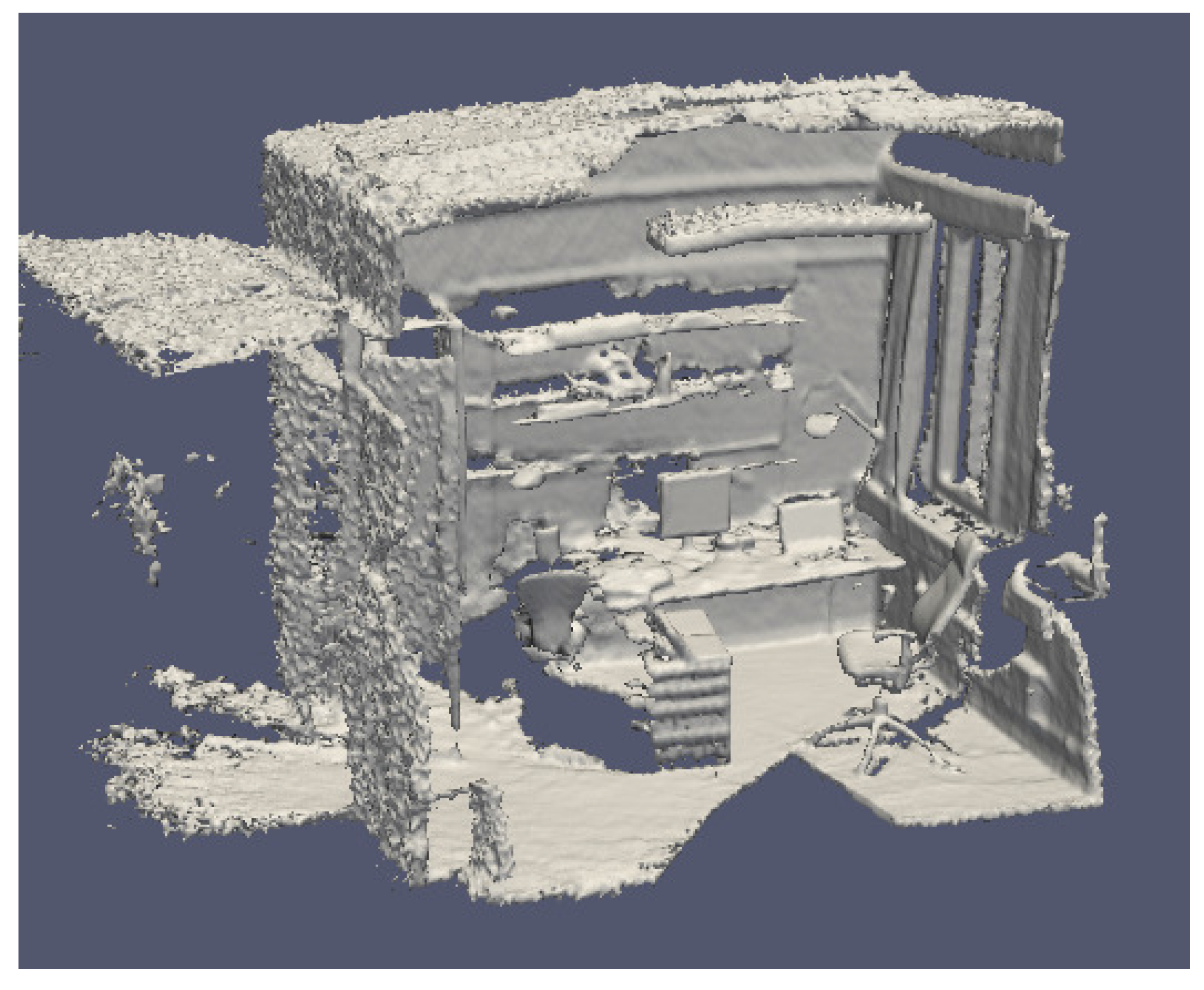
Examples from the real-world data, showing the extracted zero level set as a polygonal surface mesh. The picture depicts a partial reconstruction of a small office environment.
Figure 1.
Examples from the real-world data, showing the extracted zero level set as a polygonal surface mesh. The picture depicts a partial reconstruction of a small office environment.

Figure 2.
Examples from the synthetic data set showing a variety of shapes represented by truncated distance fields, sampled onto a small volume containing 4096 voxels.
Figure 2.
Examples from the synthetic data set showing a variety of shapes represented by truncated distance fields, sampled onto a small volume containing 4096 voxels.

Figure 3.
Example reconstruction using a PCA basis with 128 components. The reconstructed version (b) includes some blocking artifacts, visible as tiles on the floor of the room, but contains visibly less noise than the original map (a).
Figure 3.
Example reconstruction using a PCA basis with 128 components. The reconstructed version (b) includes some blocking artifacts, visible as tiles on the floor of the room, but contains visibly less noise than the original map (a).

Figure 4.
A slice through the distance field reconstructed through different methods, using 64-element encodings. Shown here are (a) the original map; (b) the Gaussian filtered map; (c) PCA reconstruction; and (d) auto-encoder reconstruction.
Figure 4.
A slice through the distance field reconstructed through different methods, using 64-element encodings. Shown here are (a) the original map; (b) the Gaussian filtered map; (c) PCA reconstruction; and (d) auto-encoder reconstruction.

Figure 5.
Selective reconstruction of floor surfaces. Given a compressed map, the minimum distance for each compressed block, to a set of descriptors that relate to horizontal planes can be computed (e.g., floors). Only the blocks that are similar enough to this set of descriptors need to be considered for actual decompression. In (a), the uncompressed map is shown, with each region colored according to its descriptor’s distance to the set of descriptors that relate to floors. In (b), we see the selectively expanded floor cells.
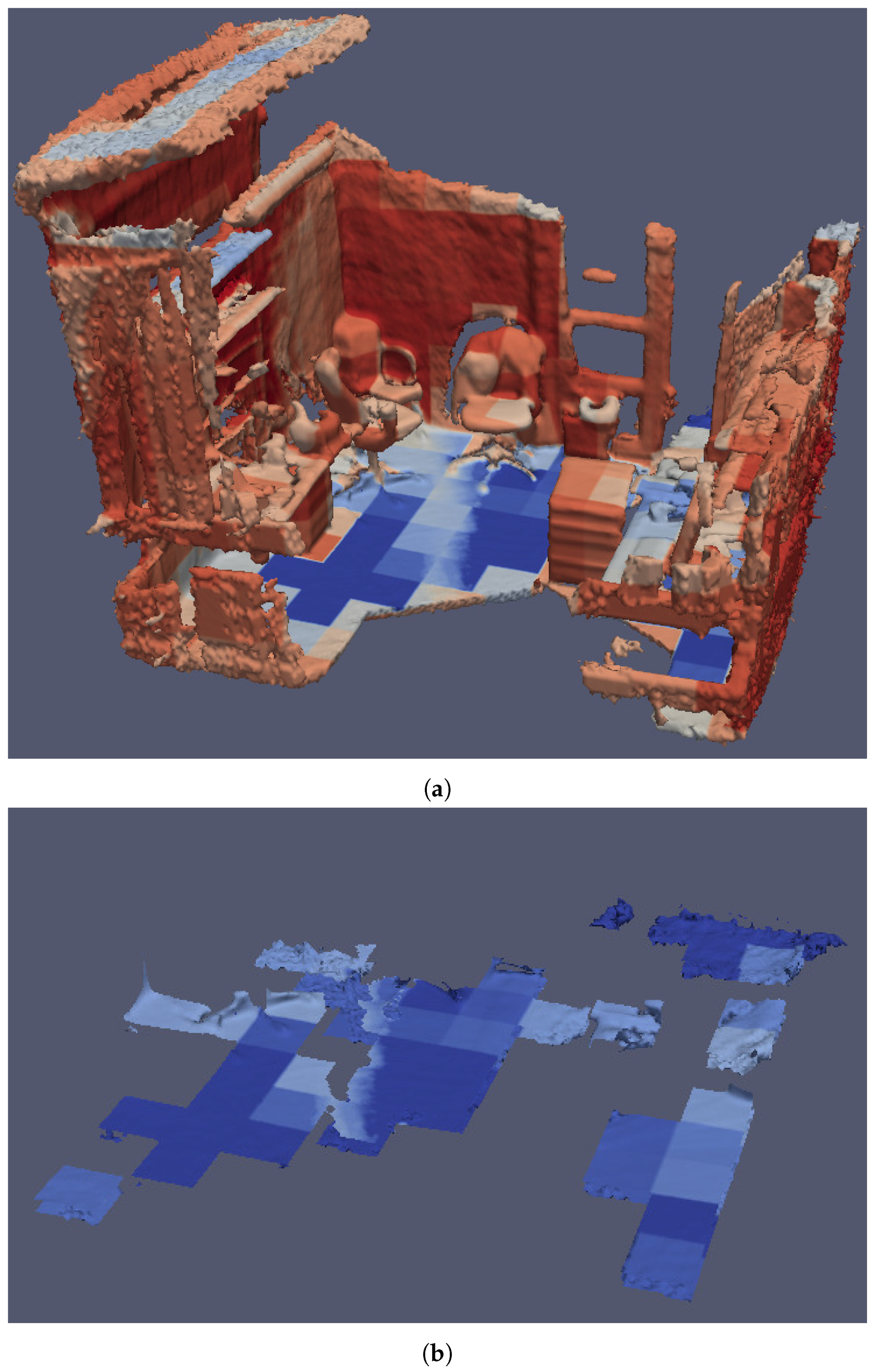
Figure 6.
Large scale mapping, enabled by real-time encoding and decoding of data as the reconstruction volume translates to keep the camera within its bounds. The active reconstruction volume is shown in black outlines. Each block is color-coded according to which descriptors it mostly resembles. In this example, we have compared the descriptors against those associated with walls and the floor, as described in the previous section.


Table 1.
Average reconstruction and ego-motion estimation results across all data sets. PCA—Principal component analysis compression, NN—Artificial neural network compression, MSE—Mean squared error, ATE—Absolute trajectory error.
Table 1.
Average reconstruction and ego-motion estimation results across all data sets. PCA—Principal component analysis compression, NN—Artificial neural network compression, MSE—Mean squared error, ATE—Absolute trajectory error.
| Reconstruction Method | Reconstruction Error (MSE) | Mean ATE [m] | Median ATE [m] |
|---|---|---|---|
| Original data | - | 0.63 ± 0.56 | 0.72 |
| PCA 32 | 42.8 ± 6.39 | 0.23 ± 0.34 | 0.049 |
| PCA 64 | 33.81 ± 3.88 | 0.36 ± 0.47 | 0.047 |
| PCA 128 | 26.88 ± 2.57 | 0.56 ± 0.68 | 0.12 |
| NN 32 | 59.66 ± 7.17 | 0.16 ± 0.29 | 0.057 |
| NN 64 | 49.18 ± 4.72 | 0.12 ± 0.17 | 0.049 |
| NN 128 | 45.66 ± 4.25 | 0.13 ± 0.20 | 0.046 |
| Gaussian Blur 9 × 9 × 9 | - | 0.10 ± 0.17 | 0.038 |
© 2017 by the authors. Licensee MDPI, Basel, Switzerland. This article is an open access article distributed under the terms and conditions of the Creative Commons Attribution (CC BY) license (http://creativecommons.org/licenses/by/4.0/).
Share and Cite
MDPI and ACS Style
Ricao Canelhas, D.; Schaffernicht, E.; Stoyanov, T.; Lilienthal, A.J.; Davison, A.J. Compressed Voxel-Based Mapping Using Unsupervised Learning. Robotics 2017, 6, 15. https://doi.org/10.3390/robotics6030015
AMA Style
Ricao Canelhas D, Schaffernicht E, Stoyanov T, Lilienthal AJ, Davison AJ. Compressed Voxel-Based Mapping Using Unsupervised Learning. Robotics. 2017; 6(3):15. https://doi.org/10.3390/robotics6030015
Chicago/Turabian StyleRicao Canelhas, Daniel, Erik Schaffernicht, Todor Stoyanov, Achim J. Lilienthal, and Andrew J. Davison. 2017. "Compressed Voxel-Based Mapping Using Unsupervised Learning" Robotics 6, no. 3: 15. https://doi.org/10.3390/robotics6030015
Note that from the first issue of 2016, this journal uses article numbers instead of page numbers. See further details here.