Trajectory Planning and Tracking Control of a Differential-Drive Mobile Robot in a Picture Drawing Application

Department of Electrical Engineering, National Taiwan University of Science and Technology, Taipei 10607, Taiwan
*
Author to whom correspondence should be addressed.
Robotics 2017, 6(3), 17; https://doi.org/10.3390/robotics6030017
Submission received: 21 June 2017
/
Revised: 7 August 2017
/
Accepted: 7 August 2017
/
Published: 10 August 2017
Abstract
:This paper proposes a method for trajectory planning and control of a mobile robot for application in picture drawing from images. The robot is an accurate differential drive mobile robot platform controlled by a field-programmable-gate-array (FPGA) controller. By not locating the tip of the pen at the middle between two wheels, we are able to construct an omnidirectional mobile platform, thus implementing a simple and effective trajectory control method. The reference trajectories are generated based on line simplification and B-spline approximation of digitized input curves obtained from Canny’s edge-detection algorithm on a gray image. Experimental results for image picture drawing show the advantage of this proposed method.
1. Introduction
Wheeled mobile robots are increasingly present in industrial, service, and educational robotics, particularly when autonomous motion capabilities are required on a smooth ground plane. For instance, [1] used image processing techniques to detect, follow, and semi-automatically repaint a half-faded lane mark on an asphalt road. Employing a mobile robot platform in drawing robot applications has the advantages of small size, large work space, portability, and low cost. A drawing robot is a robot that makes use of image processing techniques in input an image and draws the same image picture. A transitional x-y plotter has limits in terms of work space and becomes more expensive for large work sizes. Most portrait drawing robots/humanoid robots make use of multi-degrees of freedom for robot arms [2,3,4,5]. However, it may be too costly to use a robot arm in drawing a picture or portrait.
The basic motion tasks for a mobile robot in an obstacle-free work space are point-to-point motion and trajectory following. Trajectory tracking control is particularly useful in art drawing applications, in which a representative physical point (pen tip, for instance) on the mobile robot must follow a trajectory in the Cartesian space starting from an arbitrary initial posture. The trajectory tracking problem has been solved by various approaches, such as Lyapunov-based non-linear feedback control, dynamic feedback linearization, feed-forward plus feedback control, and others [6,7,8]. In this work, we propose a simple and effective trajectory control method for a picture drawing robot that is based on inverse kinematics and proportional feedback control in discrete time.
Omnidirectional motion capability is another important factor in fine and precise motion applications. Designing a mobile robot with isotropy kinematic characteristics requires three active wheels with a special wheel mechanism design [9]. Kinematic isotropy means the Jacobian matrix is isotropic for all robot poses, which is one of the key factors in robotic mechanism design [10,11]. Kinematic isotropy makes the best use of control degrees of freedom in Cartesian motion.
The standard construction of a mobile drawing robot is based on a classical differential drive chassis with the single castor in the back of the robot [12,13]. Some robots are driven by two stepper motors, in which the motor control is an open-loop control. Thus, the robot’s position and orientation are computed based on the input step command for stepper motors [13]. For most differential-drive mobile drawing robots, the draw pen is installed in the middle of the wheels; therefore, this configuration is not omnidirectional in kinematics, and a sharp curve is difficult and consumes more power to draw. The motivation of this work is, thus, to explore the omnidirectional motion capability for a two-control degrees of freedom differential-drive mobile robot platform for application in fine art drawing. When the draw pen does not stall at the middle of the wheels, a differential-drive mobile robot platform may be omnidirectional and even isotropic in the Cartesian space by not considering heading control. Moreover, the mobile platform has less power consumption for a given reference following path and possibly can be used for sharp turn motions.
For the first step toward an autonomous art drawing system, the authors propose an integral system consisting of a remote main controller and a drawing mobile robot. The remote main controller can be either a personal computer (PC) or a smartphone, which automatically generates line drawing picture data from a camera in real time. The picture curves are generated in the sequence of image edge detection, searching and sorting connected paths, line simplification of image space curves, and line curve smoothing by cubic B-spline approximation. The drawing mobile robot is equipped with a pen and wireless Bluetooth connection; thus, it is able to draw pictures on a paper on-line. The robot is an accurate mobile two-wheel differential driven robot controlled by a field programmable gate array (FPGA) controller. The robot is driven by two dc servo motors. The motor control is under closed-loop position proportional-integral-derivative (PID) control. The contributions of this work are as follows:
- (1)
- omnidirectional motion for a differential drive mobile robot platform;
- (2)
- autonomous art drawing system can be built to keep both mobile robot platform and control algorithm as simple as possible; and
- (3)
- system integration of a mobile pen drawing platform by image edge detection, line simplification and smoothing, trajectory following control, and FPGA controller.
The rest of the paper is organized as follows: Section 2 presents an omnidirectional model of a differential-drive mobile robot. Section 3 shows trajectory tracking control methods and stability analysis. Section 4 studies trajectory planning for drawing a connected digitized curve through line simplification and line smoothing. Section 5 illustrates searching and sorting picture curves of a gray image. Section 6 provides both simulation and experimental results obtained from a test-bed mobile robot. Section 7 concludes the paper.
2. Kinematic Model of a Differential-Drive Mobile Platform
This study considers a simple mobile robot platform with two independent driving wheels and one castor free wheel. A draw pen is installed along a perpendicular line between the middle of the two wheels to depict an image picture. Let be driving the wheel angular velocity, is the radius of the driving wheel, is half of the distance between the two wheels, and D is the perpendicular distance from the pen position to the middle of the two wheels, as shown in Figure 1. We define as the position of the middle of the two wheels and as the tip position of the pen in the world frame {W}. The origin of the robot base frame {B} is assigned to the middle of two wheels, and is the mobile robot yaw angle and is the orientation angle from pointing to relative to the x-axis of the world reference frame {W}, as shown in Figure 1.
Let and be the instantaneous linear velocity of the origin and angular velocity of the robot base frame, respectively. The velocity kinematic equation of the mobile robot platform is represented by
and
Common to all types of mobile robots with two control degrees of freedom, this kinematic is not-omnidirectional. Suppose that the Cartesian position of the pen is the representative point of the mobile robot platform,
and hence,
The mobile robot platform kinematics without heading control is now defined by
where the Jacobian matrix is
where ratio . The determinant of the Jacobian matrix, , is a constant. Therefore, by not locating the pen at the middle of the wheels, i.e., , the Jacobian matrix is well-conditioned and the inverse Jacobian matrix is
It is clear that the control degree in the yaw angle is now transformed to the control degree in the lateral linear motion. The bigger the is, the larger the mobility is in the lateral motion. Without consideration of the orientation angle, the mobile robot platform becomes an omnidirectional platform in the Cartesian space. An interesting example is a circular shape robot with a pen installed at the center position.
The singular value decomposition of the Jacobian matrix is
where
and
The maximum and minimum singular values of the Jacobian matrix are and , respectively; and the condition number . When , the condition number equals one, and the columns of the Jacobian matrix are orthogonal and of equal magnitude for all robot poses. Thus, the mobile robot platform and pen system exhibit kinematic isotropy. Each wheel causes the pen’s motion to be of equal amount and orthogonal to that caused by the other wheel. In this case, it makes the best use of the degrees of freedom of the two wheels in the Cartesian motion.
3. Mobile Platform Trajectory Tracking Control Methods
3.1. Trajectory Tracking Control and Stability
As stated above, the tip position of the pen is the representative point of the mobile robot platform, which must follow a referenced Cartesian trajectory , , in the presence of initial error. Since the Jacobian matrix is well-conditioned for all poses, a simple inverse kinematics-based resolved rate plus proportional control law is applied to meet the requirement for the pen trajectory control problem.
We define and as the trajectory tracking errors. The control rule of resolved rate plus P control is as follows
where is the estimated orientation angle , and and are positive gains, . Let , and then , and the error dynamics become a linear time-varying system as follows
The stability and properties of the above closed-loop system are discussed in the following two cases.
Case 1: Global exponential stability
In the case of (point-to-point motion without heading control), the closed system has a globally exponentially stable equilibrium at . It is based on the use of the Lyapunov function , , whose time derivative, , , provides that and .
Case 2: Input-to-state stability (bounded-input bounded-state stability)
Because of the bounded velocity capability of motors, the trajectory tracking velocity is limited. Assume that the derivatives of reference trajectory are limited, such that and , where m is a constant upper boundary. Lemma 4.6 of Reference [14] states that an unforced system whose trivial solution is globally exponentially stable is input-to-state stable (ISS) if submitted to a bounded input (or perturbation). Therefore, the closed system in Equation 9 is bounded-input bounded-state (BIBS) stable. Furthermore, the bounds of trajectory tracking errors are approximately and , respectively. The trajectory following errors and are directly proportional to trajectory speed m, measure error , and gains and .
3.2. Discrete-Time Trajectory Following Control Method
It is desirable to implement the above continuous-time trajectory control method in discrete-time form. Let be the trajectory control update time, and is the referenced pen trajectory at discrete time k; therefore, it is likely to generate incremental motion commands and , such that
where
and
The above inverse kinematic equation can be rewritten as
where
Here, it is assumed that and , in which is an upper boundary on how far to move the pen in a single update time. If is too distant from , then it needs to move the target position in closer to the current pen location by inserting one or more intermediate points. Control terms and can be obtained as follows
and
Motor incremental position commands are then given by
It is also required that and , where is the maximum incremental position command of each driving motor. Here, and are summed up and then used as absolute reference position commands of wheel motors, which are then sent to independent PID position controllers to close the dc motor servo control loops. Figure 2 shows the system block diagram of the proposed pen trajectory following control method. In this study, the trajectory control update time is = 20 milliseconds, and the position servo control sampling time is = 1.0 milliseconds.
The above trajectory control loop requires information from the mobile robot’s position and yaw angle. The computation of the mobile robot’s position and yaw angle is based on odometric prediction from motor encoders. The odometry update time is also chosen as = 20 milliseconds. The mobile robot’s incremental motion changes are calculated from motor encoders reading and
where
The mobile robot base position and orientation angle are updated according to
and
Robot localization using the above odometry, commonly referred to as dead reckoning, is usually accurate enough in the absence of wheel slippage and backlash.
4. Line Simplification and B-Spline Smoothing
This work represents each desired picture curve by a B-spline approximation of a digitized two-dimensional image curve , , . Here, the B-spline curves of degree 1 and degree 3 are used most often. The problem statement is depicted as follows.
Given a digitized image curve of N connected pixels , , in order to find a two-dimensional B-spline curve of degree d,
for (n + d − 1) control points , , it is best to approximate the sequence of input data points in a least-squares sense. The functions of are the B-spline basis functions, which are defined recursively as:
where , and is defined.
The B-spline curve is then the desired pen drawing reference trajectory at discrete-time t in the unit of trajectory control sampling time .
4.1. Line Simplification and Knot Section
The above B-spline approximation problem involves knot selection and control point selection. To simplify the solution search, knot selection and control point selection are found separately in two phases. Initially, the start and end knots are set to and . First, the line simplification technique is applied to select knots , , so that and . The least-squares error method is then followed to search out new control points for the purpose of line smoothing.
Line simplification is an algorithm for reducing the number of points in a curve that is approximated by a series of points within an error of epsilon. There are many line simplification algorithms—among them, the Douglas–Peucker algorithm is the most famous line simplification algorithm [15]. The starting curve is an ordered set of points or lines and the distance dimension epsilon. The algorithm recursively divides the line. It is initially given all the points between the first and last points. It automatically marks the first and last points to be kept. It then finds the point that is furthest from the line segment with the first and last points as end points; this point is obviously furthest on the curve from the approximating line segment between the end points. If the point is closer than epsilon to the line segment, then any points not currently marked to be kept can be discarded without the simplified curve being worse than epsilon. After the line simplification algorithm, the selected knots , , are built from the index of line simplification points.
A linear spline approximation of the input image curve can be obtained based on the selected knots and control points selected from those in the input dataset . The desired linear spline trajectory is then:
4.2. B-Spline Control Point Selection
This study develops the B-spline with degree d approximation of input data , , with distinct knots , , obtained from line simplification for line smoothing. First, we define open integer knots here so that , where knots and repeat (d + 1) times, in order to guarantee that the start and end points of the B-spline curve are the first and last input data and , respectively. The B-spline curves of degree 1 and degree 3 are considered in this study.
(1) B-spline of degree 1 (d = 1)
The control points are arranged here such that and to guarantee that the start and end points of the picture curve are unchanged, and (n − 2) control points are left to be determined.
(2) B-spline of degree 3 (d = 3)
The control points are arranged here such that and to guarantee zero end speeds at the start point and end point , and (n − 2) control points are left to be determined.
Control points are selected by least-squares fitting of the data with a B-spline curve:
For B-spline of degree 1 (d = 1), the fitting equations are:
Let and , and then we have an over-determined matrix equation:
where , , and .
For B-spline of degree 3 (d = 3), the fitting equations are:
Let and , and then we also have the same dimensions for an over-determined matrix equation:
where , , and .
The least-squares error solution can then be solved from the following normal equation:
or obtained from the pseudo-inverse solution:
Since the normal equation matrix is a symmetric and banded matrix, it is, therefore, desirable to search for control points through basic row eliminations and then follow with backward substitution. Once control points are found, the desired B-spline reference trajectory is generated through DeBoor’s B-spline recursive formulation [16].
5. Picture Curves Generation
We now describe the process from the input of the image picture to the desired picture curves’ generation. Picture curves are generated after Canny’s edge detection algorithm is performed on the input picture gray image [17]. The generation of picture draw curves involves searching and sorting picture curves in two stages. The strategy for searching out picture curves runs in three phases as stated below:
- Phase 1: remove salt points and branch points;
- Phase 2: search connected paths; and
- Phase 3: search loop paths.
The picture point decision is based on the local information of its adjacent pixels in a 3-by-3 window, , defined here. Let the terms 4-connect and 8-connect of a pixel point be the numbers of its 4-connected pixel equal to 1 and its 8-connected pixel equal to 1, respectively.
In phase 1, salt point and branch point are classified as below:
- salt point: 8-connect = 0; and
- branch point: 4-connect > 2.
In phase 2, start point, mid-point, and end point of a connected path are classified as below:
- start point: 4-connect = 1 or (4-connect = 0 and 8-connect = 1);
- mid-point: in the order of (P1 = 1) or (P2 = 1) or (P3 = 1) or (P4 = 1) or (P5 =1) or (P6 = 1) or (P7 = 1) or (P8 = 1);
- end point: 8-connect = 0.
In phase 3, salt point and point in a loop path are classified as below:
- salt point: 8-connect = 0;
- point in a loop path: 8-connect ≥ 2.
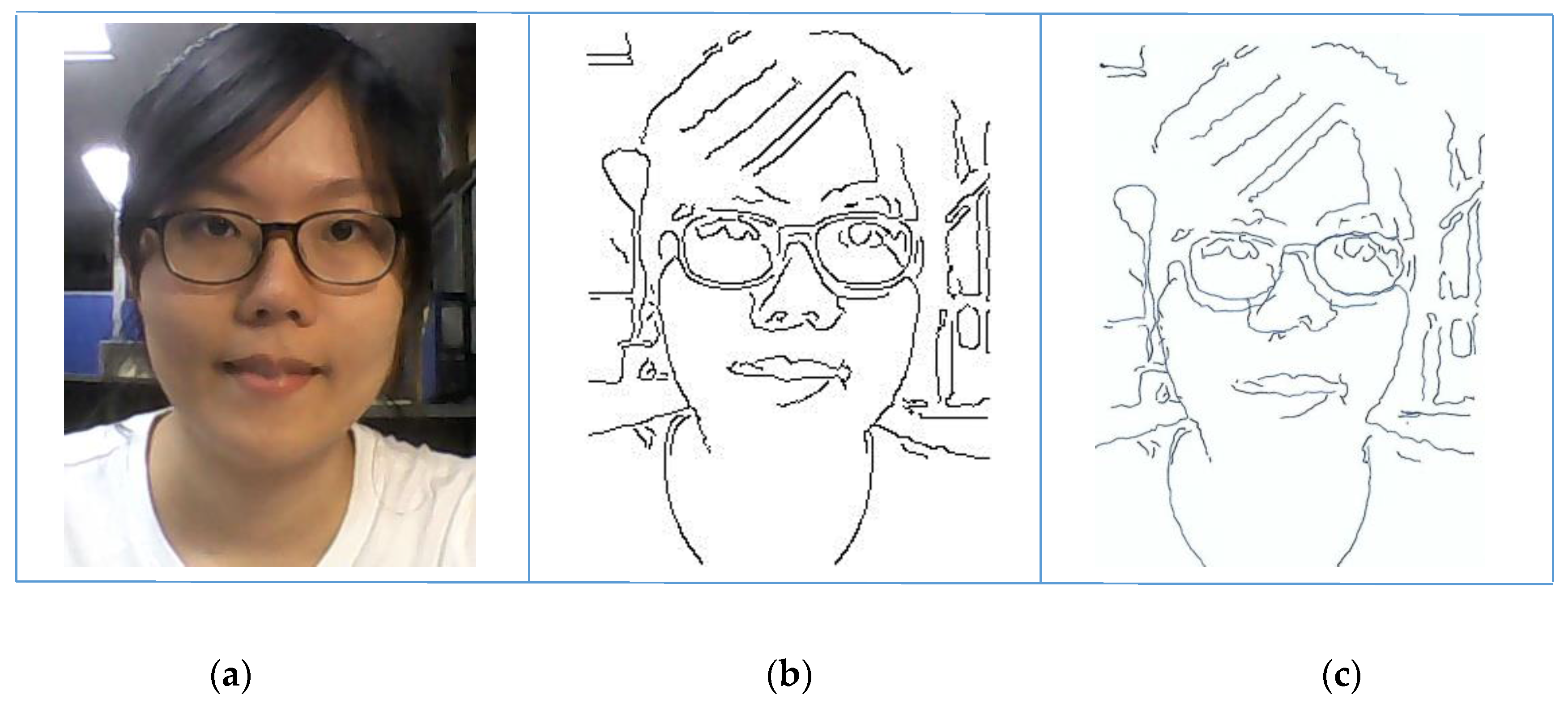
For the sorting of final picture curves, a simple greedy method of the nearest neighbor strategy is applied to sort picture curves in order to send out to the robot drawer. The next curve to be drawn is the one where one of its end points is closest to the end position of the drawing curve among the rest of the curves. Figure 3 shows picture curve search results; the input gray image has a size of 213 × 315 bytes. There are 5878 edge pixels after edge detection, and there are 136 connected curves in curve sorting. After line simplification, there are 2702 control points left.
6. Simulation and Experimental Results
The experimental autonomous robot image figure drawing system consists of a PC or a smartphone as a main controller and a differential-drive mobile robot platform as shown in Figure 4. The radius of the driving wheel is r = 56.25 mm, and the distance of two driving wheels is 2 L, where L = 12.25 mm. The wheel is actuated by a dc motor (motor maximum no-load speed 4290 rpm) with a 15:1 gear reducer, and the motor encoder has a resolution of 30,000 ppc. The proposed pen trajectory following control system is built on an Altera DE0-nano FPGA development board running at a system clock rate of 50 MHz. All control and series communication modules are implemented using Verilog hardware description language (HDL) and synthesized by an Altera Quartus II EDA tool. The image processing and connected curve generation program are programmed in Visual C++ for PC and in JAVA for smartphone. The mobile robot receives real-time picture curves data, which are generated from a PC or a smartphone through Bluetooth rs232 at a Baud-rate of 115,200 Hz.
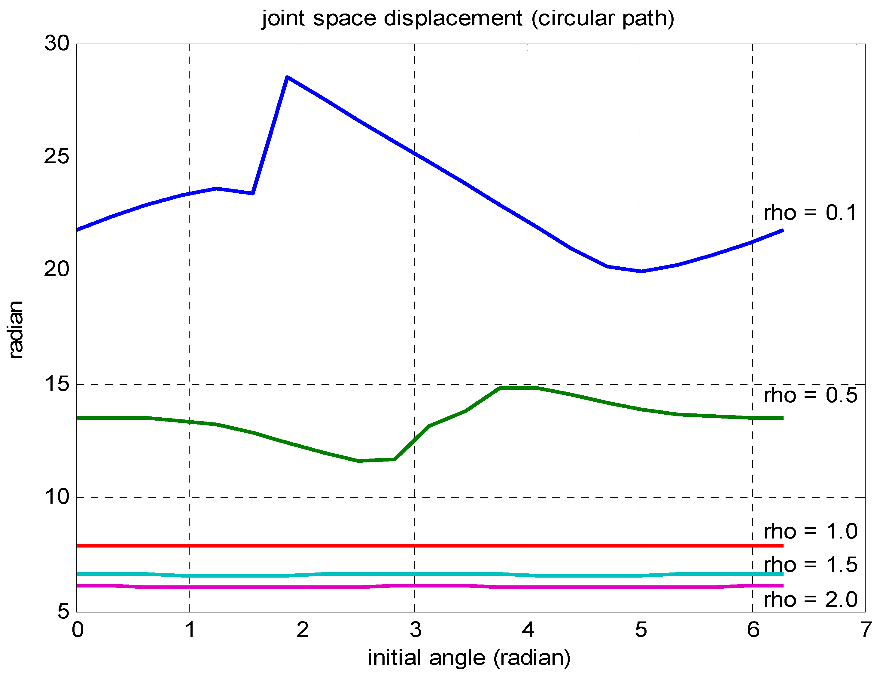
The first example considers a circular path to verify the effect of . The desired reference path trajectory is represented by and , , where R = 50 mm, and the total circular length is = 100p mm. The control law in Equation (8) with proportional gains is used. Figure 5 shows the total displacement in the joint space with respect to arbitrary initial yaw angle for several different pen location distances D to follow the desired circular path trajectory.
The second example considers a square path of side length 100 mm, and the total length is = 400 mm. Figure 6 shows the total displacement in the joint space with respect to initial angle yaw for several different pen location distances D to follow the desired square path trajectory. As expected, the joint space displacement decreases as the distance D increases. When (i.e., D = L), the Jacobian matrix is isotropic for all mobile robot poses; and hence, is independent on the mobile robot initial yaw angle and .
In the following trajectory control experiments, a drawing pen is located at a distance of D = 50 mm. The discrete-time trajectory following control law in Equations (11) and (12) is applied with trajectory and feedback update time = 0.01 s. Figure 7 and Figure 8 show the experimental mobile robot’s drawn results of a circular path (radius 50 mm) and a square path (side length 100 mm), respectively. For both curves, the trajectory following error is within 3.0 mm without initial position error. It is shown that the pen tip trajectory has small trajectory tracking errors in sharp turn corners in Figure 8.
Figure 9 shows the experimental drawn results of Taiwan maps. The origin data has 1105 discrete data points, and there are 42 control points in its line simplification curve, and 44 control points in the cubic B-spline smoothing curve. Figure 10 shows tracking errors of drawn Taiwan maps in Figure 9. The drawing size is 160 × 80 mm2, tracking errors are within 1.0 mm, and drawing time is 10 s. Since the step size is small, there are few differences in Figure 10.
Figure 11 shows the drawn results of a building image in Figure 3, in which there are 136 connected curves with 2702 control points in total after procedures of edge detection and line simplification. The drawing size is 150 × 120 mm2 and drawing time is about 90 s.
Figure 12 shows the image drawn by the experimental mobile robot of a human portrait. The original image is 280 × 210 pixels and has 3951 pixels after edge detection, and it leaves 100 connected curves with 2267 control points after line simplification. The drawn picture size is 8.0 × 5.0 cm2 and is done in about 60 s.
7. Conclusions
What is new in this present research is that by removing the control degree in yaw angle to a linear lateral motion of a differential-drive mobile robot, an omnidirectional platform can be built. Thus, we can design an autonomous art drawing platform in a closed-loop fashion through an inverse kinematics plus proportional control approach. Both simulation and experimental results show that the experimental system works in practice as well as in theory. The limitations of the current system are a lack of heading control in trajectory tracking control and slower motion of the mobile system. Further works can include integrating the vision system in the FPGA, refining the mobile robot odometry for longer traveling distance, and developing fast speed motion controller.
Acknowledgments
This work is supported by grants from Taiwan’s Ministry of Science and Technology, MOST 105-2221-E-011-047 and 106-2221-E-011-151.
Author Contributions
C.-L. Shih and L.-C. Lin conceived and designed the experiments; L.-C. Lin performed the experiments; C.-L. Shih and L.-C. Lin analyzed the data; C.-L. Shih wrote the paper.
Conflicts of Interest
The authors declare no conflict of interest.
References
- Kotani, S.; Yasutomi, S.; Kin, X.; Mori, H.; Shigihara, S.; Matsumuro, Y. Image processing and motion control of a lane mark drawing robot. In Proceedings of the IEEE/RSJ International Conference on Intelligent Robots and Systems, Yokohama, Japan, 26–30 July 1993; pp. 1035–1041. [Google Scholar]
- Srikaew, A.; Cambron, M.; Northrup, S.; Peters, R.A., II; Wilkes, M.; Kawamura, K. Humanoid drawing robot. In Proceedings of the IASTED International Conference on Robotics and Manufacturing, Banff, AB, Canada, 26–29 July 1998. [Google Scholar]
- Lau, M.C.; Baltes, J.; Anderson, J.; Durocher, S. A portrait drawing robot using a geometric graph approach: Furthest Neighbour Theta-graphs. In Proceedings of the IEEE/ASME International Conference on Advanced Intelligent Mechatronics (AIM), Kachsiung, Taiwan, 11–14 July 2012; pp. 75–79. [Google Scholar]
- Tresset, P.; Leymarie, F.F. Portrait drawing by Paul the robot. Comput. Gr. 2013, 37, 348–363. [Google Scholar] [CrossRef]
- Jain, S.; Gupta, P.; Kumar, V.; Sharma, K. A force-controlled portrait drawing robot. In Proceedings of the IEEE International Conference on Industrial Technology (ICIT), Seville, Spain, 17–19 March 2015; pp. 3160–3165. [Google Scholar]
- Kanayama, Y.; Kimura, Y.; Miyazaki, F.; Noguchi, T. A stable tracking control method for an autonomous mobile robot. In Proceedings of the IEEE International Conference on Robotics and Automation, Cincinnati, OH, USA, 13–18 May 1990; pp. 384–389. [Google Scholar]
- Samson, C. Control of chained systems application to path following and time-varying point-stabilization of mobile robots. IEEE Trans. Autom. Control 1995, 40, 64–77. [Google Scholar] [CrossRef]
- Egerstedt, M.; Hu, X.; Stotsky, A. Control of mobile platforms using a virtual vehicle approach. IEEE Trans. Autom. Control 2001, 46, 1777–1782. [Google Scholar] [CrossRef]
- Saha, S.K.; Angeles, J.; Darcovich, J. The kinematic design of a 3-DOF isotropic mobile robot. In Proceedings of the IEEE International Conference on Robotics and Automation, Atlanta, GA, USA, 2–6 May 1993; pp. 283–288. [Google Scholar]
- Togai, M. An application of singular value decomposition to manipulability and sensitivity of industrial robots. SIAM J. Algebraic Discret. Methods 1986, 7, 315–320. [Google Scholar] [CrossRef]
- Merlet, J.-P. Jacobian, manipulability, condition number and accuracy of parallel robots. ASME J. Mech. Des. 2006, 128, 199–206. [Google Scholar] [CrossRef]
- Durina, D.; Petrovic, P.; Balogh, R. Robotnacka—The drawing robot. Acta Mech. Slov. 2006, 10, 113–118. [Google Scholar]
- Balogh, R. Practical kinematics of the differential driven mobile robot. Acta Mech. Slov. 2007, 11, 11–16. [Google Scholar]
- Khalil, H.K. Nonlinear Systems, 3rd ed.; Prentice-Hall: Upper Saddle River, NJ, USA, 2002. [Google Scholar]
- Douglas, D.H.; Thomas, K.; Peucker, T.K. Algorithms for the reduction of the number of points required to represent a digitized line or its caricature. Can. Cartogr. 1973, 10, 112–122. [Google Scholar] [CrossRef]
- De Boor, C. A Practical Guide to Splines, revised version; Springer: New York, NY, USA, 2001. [Google Scholar]
- Canny, J. A Computational Approach to Edge Detection. IEEE Trans. Pattern Anal. Mach. Intell. 1986, 8, 679–698. [Google Scholar] [CrossRef] [PubMed]
Figure 1.
Coordinate frames of the mobile robot platform and pen system: the world frame {W} and robot base frame {B} with origin at the middle of two wheels. A draw pen is installed along a perpendicular line between the middle of the two wheels.
Figure 1.
Coordinate frames of the mobile robot platform and pen system: the world frame {W} and robot base frame {B} with origin at the middle of two wheels. A draw pen is installed along a perpendicular line between the middle of the two wheels.
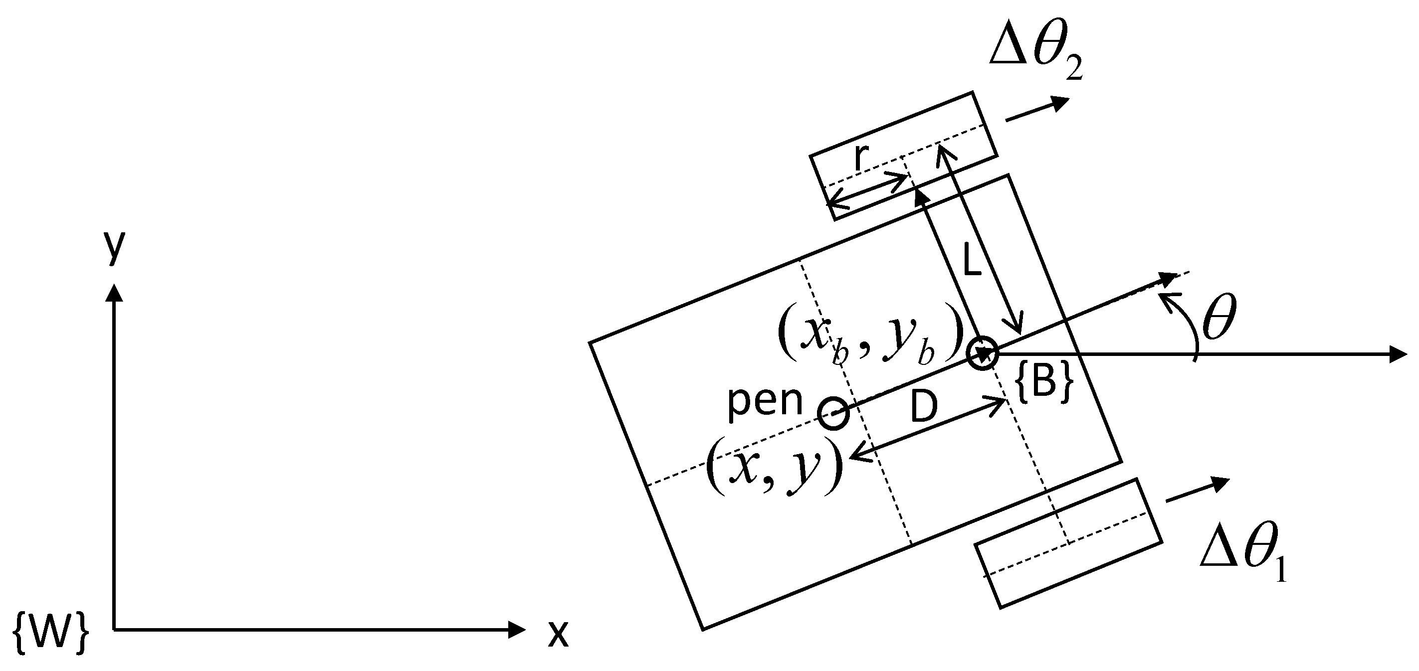
Figure 2.
The system block diagram of the pen trajectory following control.
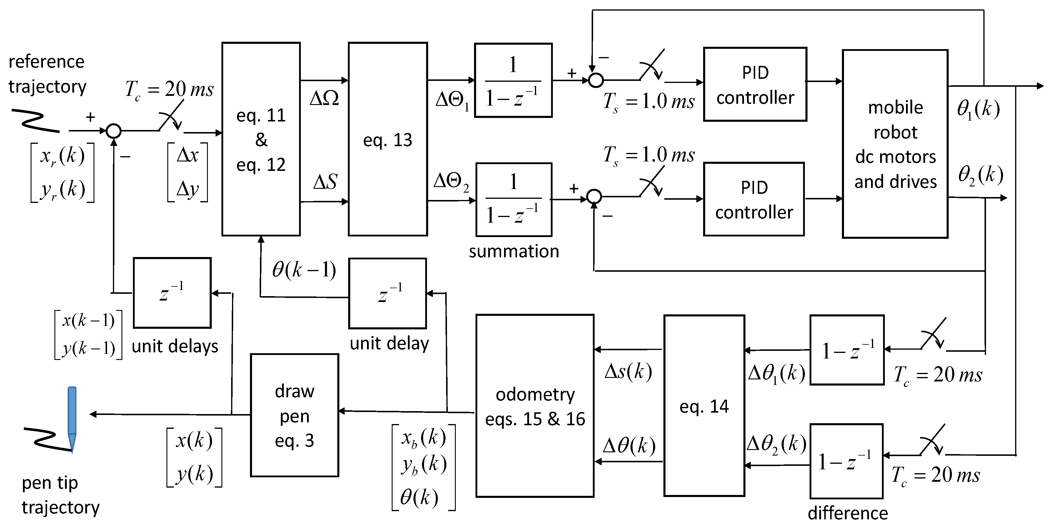
Figure 3.
Image picture curves search results: (a) original image; (b) edge detection results; and (c) searched picture curves.
Figure 3.
Image picture curves search results: (a) original image; (b) edge detection results; and (c) searched picture curves.
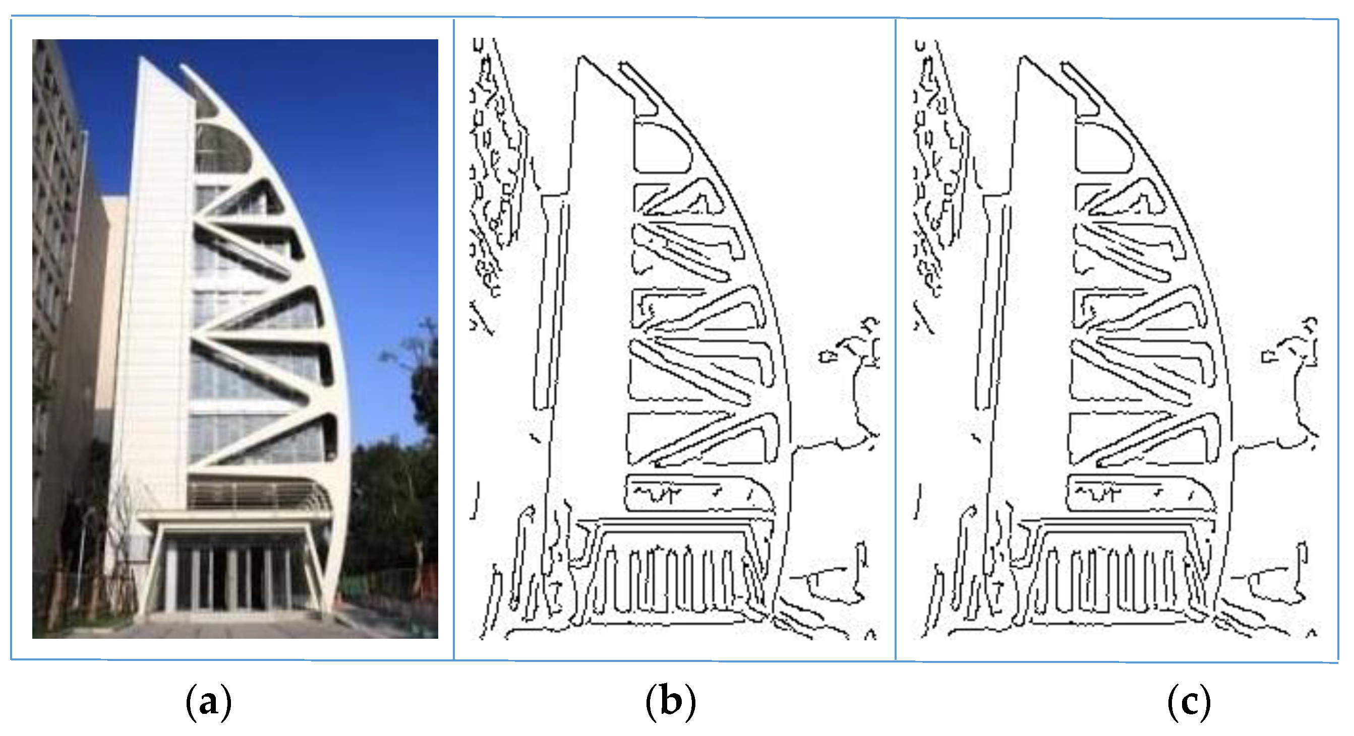
Figure 4.
A differential-drive mobile robot platform with a draw pen to generate a picture from an image.
Figure 4.
A differential-drive mobile robot platform with a draw pen to generate a picture from an image.
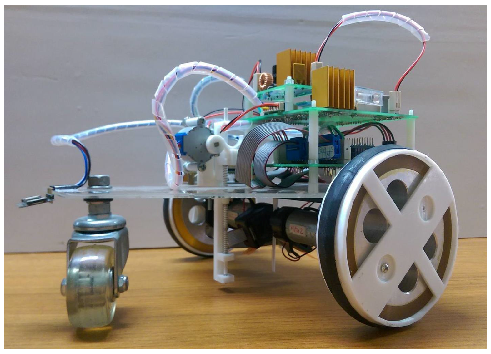
Figure 5.
Simulation results of the effect of for a differential-drive mobile robot to follow in a circular path.
Figure 5.
Simulation results of the effect of for a differential-drive mobile robot to follow in a circular path.

Figure 6.
Simulation results of the effect of for a differential-drive mobile robot to follow in a square path.
Figure 6.
Simulation results of the effect of for a differential-drive mobile robot to follow in a square path.
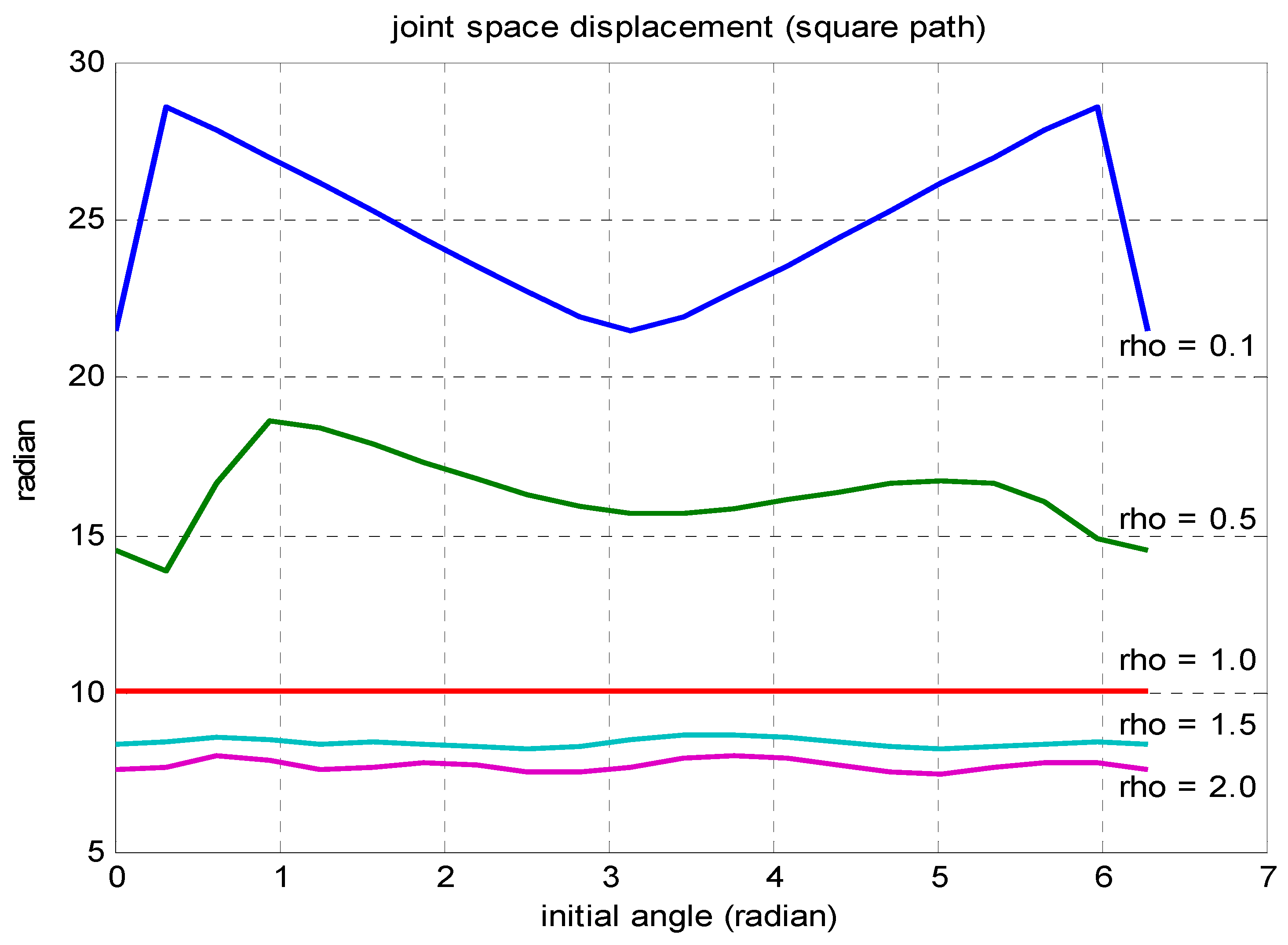
Figure 7.
Experimental drawn results of the pen tip trajectory following control of a circular path with a radius of 50 mm. (a) desired and drawn circular paths; (b) tracking error and orientation angle.
Figure 7.
Experimental drawn results of the pen tip trajectory following control of a circular path with a radius of 50 mm. (a) desired and drawn circular paths; (b) tracking error and orientation angle.
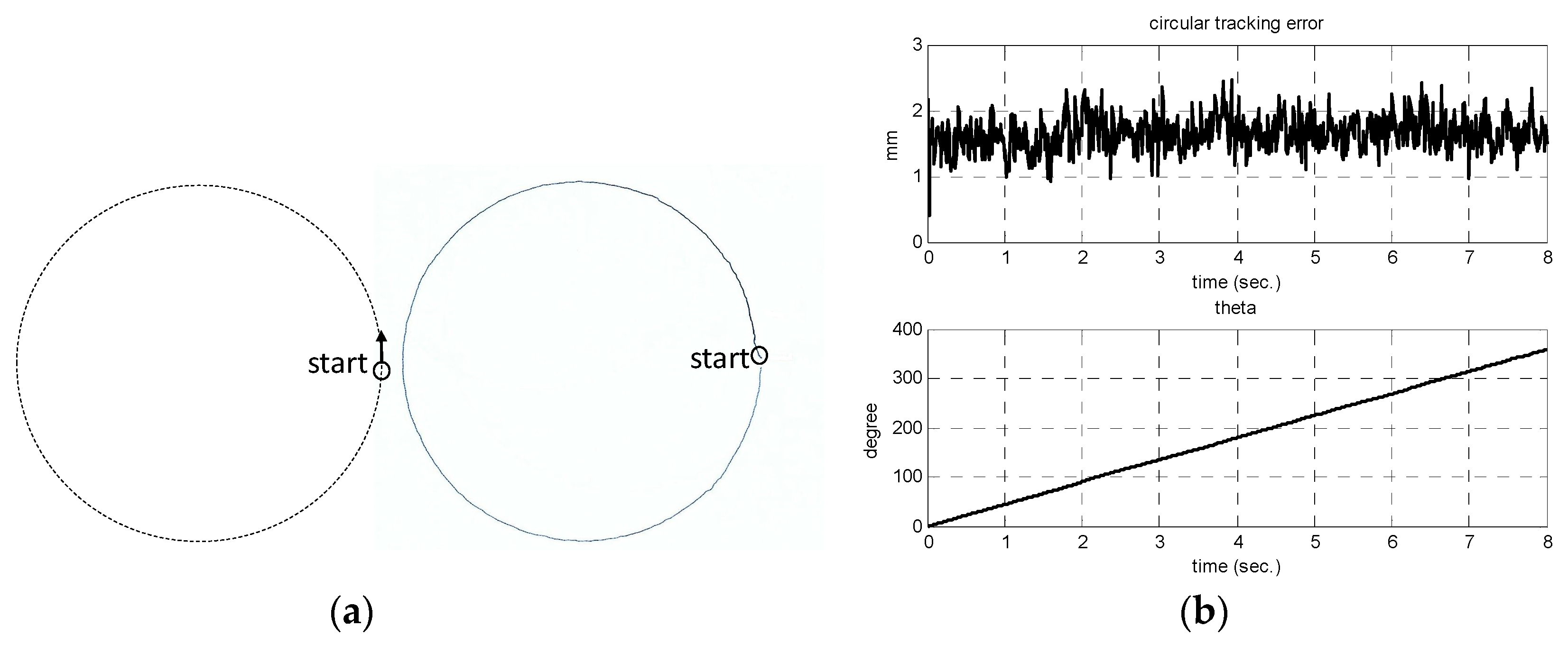
Figure 8.
Experimental drawn results of the pen tip trajectory following control of a square curve path with side lengths of 100 mm. (a) desired and drawn square paths; (b) tracking error and orientation angle.
Figure 8.
Experimental drawn results of the pen tip trajectory following control of a square curve path with side lengths of 100 mm. (a) desired and drawn square paths; (b) tracking error and orientation angle.
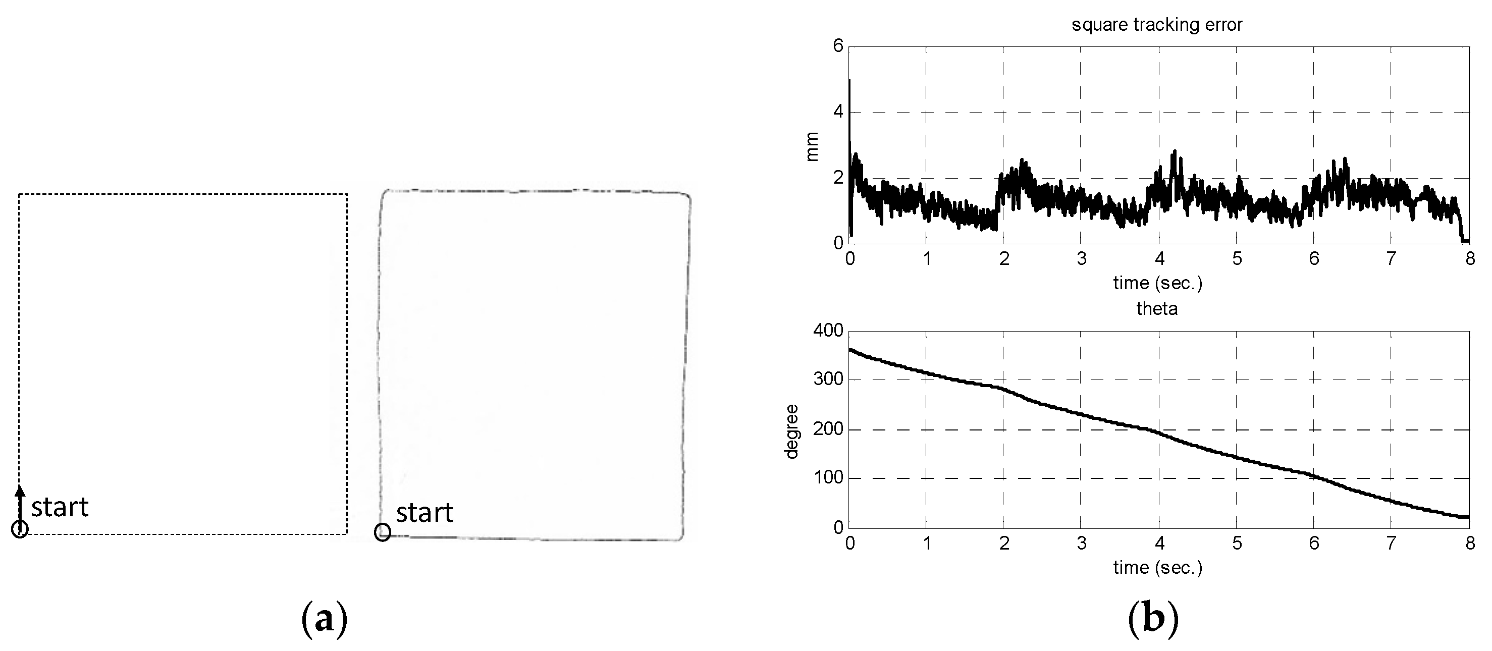
Figure 9.
Experimental drawn results of Taiwan maps: (a) original map; (b) desired line simplification curve; (c) desired cubic B-spline curve; (d) drawn Taiwan map (from line simplification) and (e) drawn Taiwan map (from line smoothing).
Figure 9.
Experimental drawn results of Taiwan maps: (a) original map; (b) desired line simplification curve; (c) desired cubic B-spline curve; (d) drawn Taiwan map (from line simplification) and (e) drawn Taiwan map (from line smoothing).
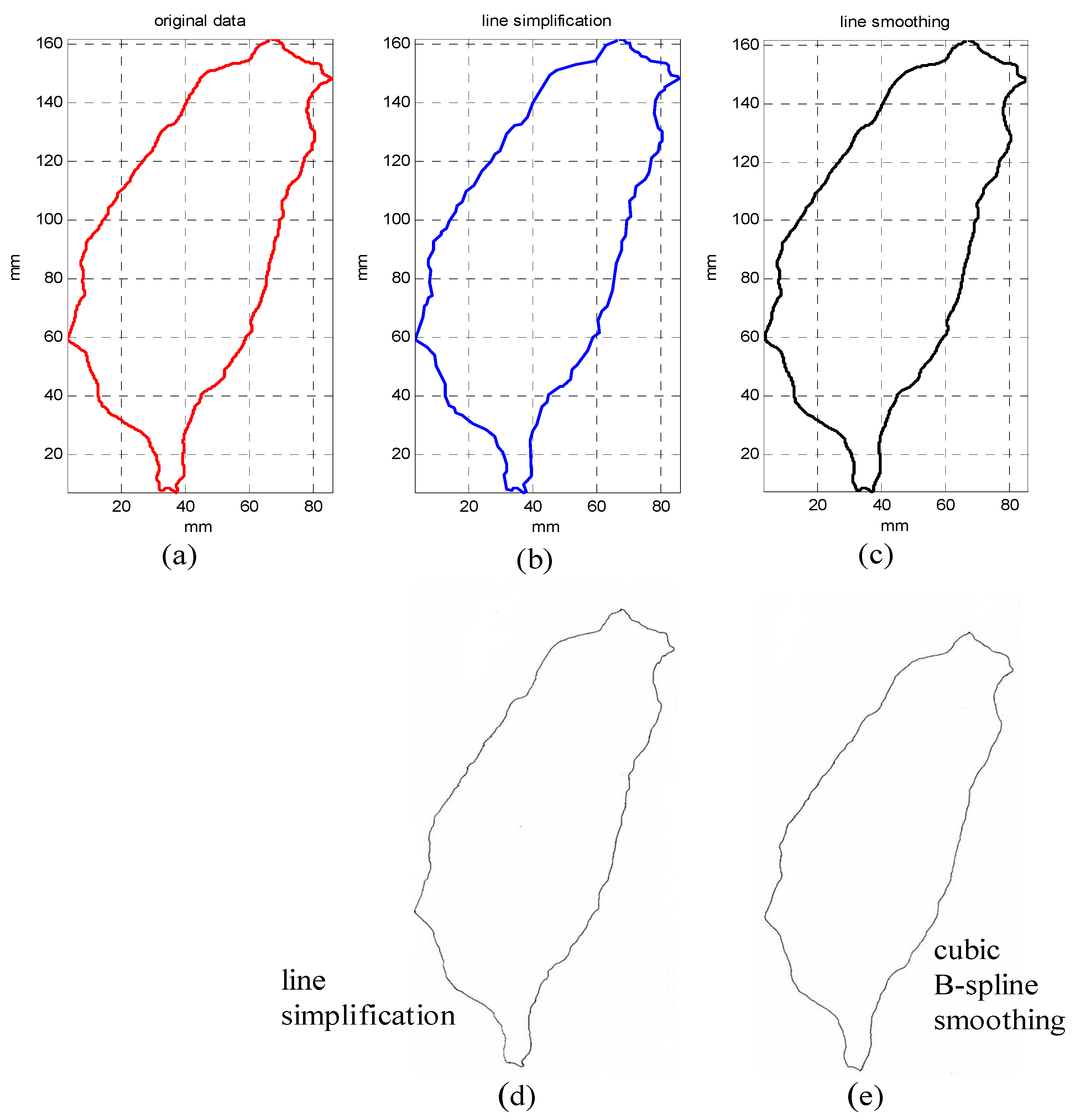
Figure 10.
Tracking errors of drawn Taiwan maps in Figure 9d,e.
Figure 10.
Tracking errors of drawn Taiwan maps in Figure 9d,e.
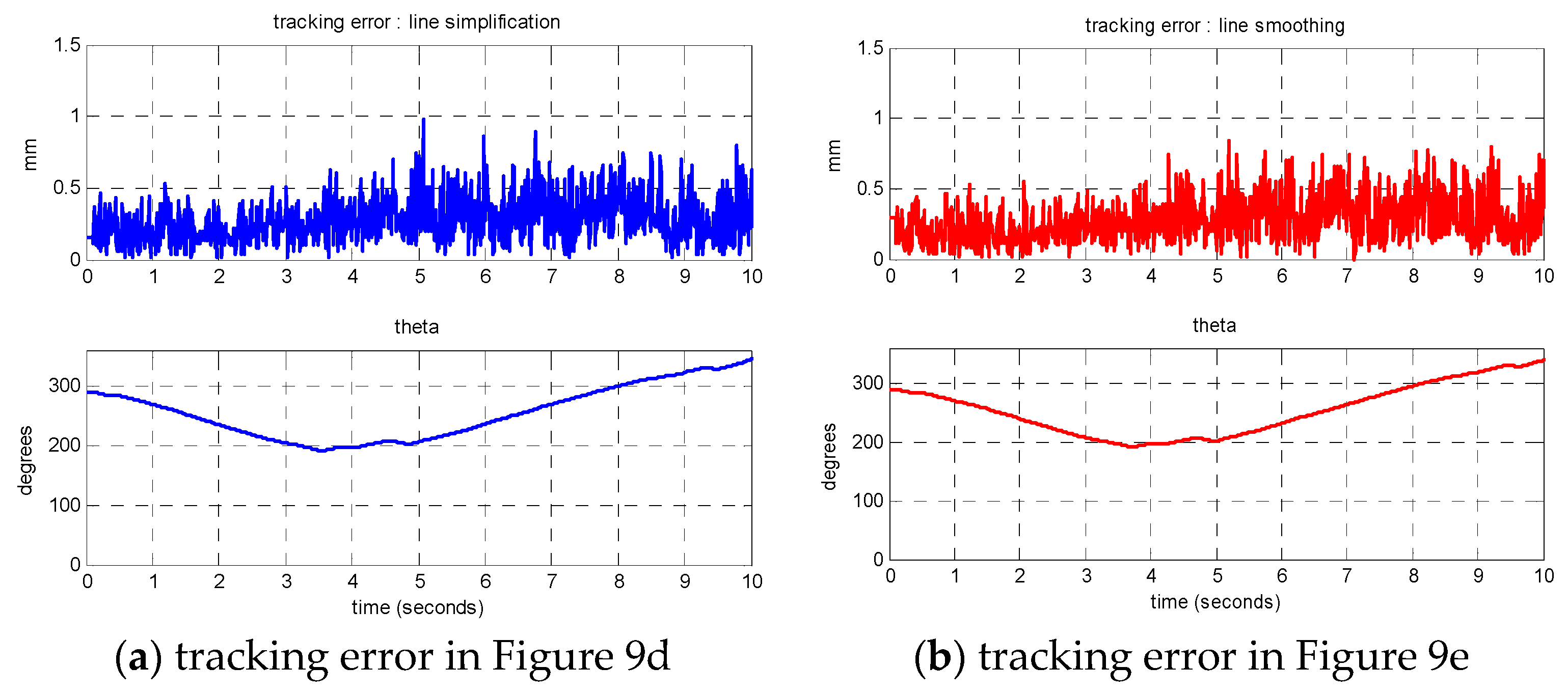
Figure 11.
Drawn result of a building image compared to (a) the original image; (b) searched picture curves; and (c) drawn picture.
Figure 11.
Drawn result of a building image compared to (a) the original image; (b) searched picture curves; and (c) drawn picture.
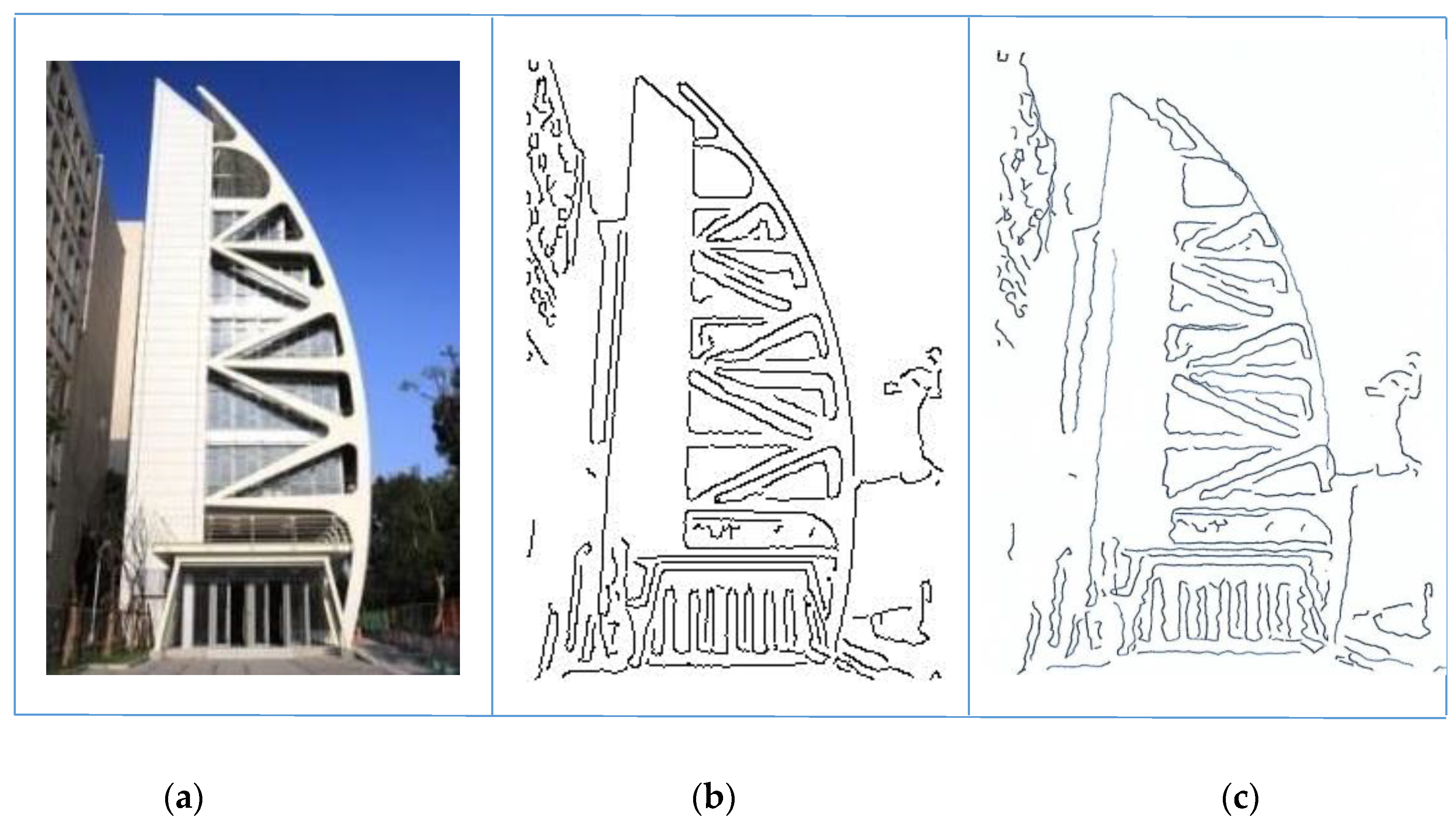
Figure 12.
Image drawn by the mobile robot is compared to (a) the original image; (b) searched picture curves; and (c) drawn picture.
Figure 12.
Image drawn by the mobile robot is compared to (a) the original image; (b) searched picture curves; and (c) drawn picture.

© 2017 by the authors. Licensee MDPI, Basel, Switzerland. This article is an open access article distributed under the terms and conditions of the Creative Commons Attribution (CC BY) license (http://creativecommons.org/licenses/by/4.0/).
Share and Cite
MDPI and ACS Style
Shih, C.-L.; Lin, L.-C. Trajectory Planning and Tracking Control of a Differential-Drive Mobile Robot in a Picture Drawing Application. Robotics 2017, 6, 17. https://doi.org/10.3390/robotics6030017
AMA Style
Shih C-L, Lin L-C. Trajectory Planning and Tracking Control of a Differential-Drive Mobile Robot in a Picture Drawing Application. Robotics. 2017; 6(3):17. https://doi.org/10.3390/robotics6030017
Chicago/Turabian StyleShih, Ching-Long, and Li-Chen Lin. 2017. "Trajectory Planning and Tracking Control of a Differential-Drive Mobile Robot in a Picture Drawing Application" Robotics 6, no. 3: 17. https://doi.org/10.3390/robotics6030017
Note that from the first issue of 2016, this journal uses article numbers instead of page numbers. See further details here.