Proposal of Novel Model for a 2 DOF Exoskeleton for Lower-Limb Rehabilitation


1
Faculty of electronics Engineering, Universidad Santo Tomás, Bogotá 110311, Colombia
2
Departamento de Ingeniería Eléctrica y Electrónica, Universidad Nacional de Colombia, Bogotá 110311,Colombia
3
Faculty of Engineering, Fundación Universitaria Los Libertadores, Bogotá 110311, Colombia
*
Author to whom correspondence should be addressed.
Robotics 2017, 6(3), 20; https://doi.org/10.3390/robotics6030020
Submission received: 21 June 2017
/
Revised: 13 August 2017
/
Accepted: 31 August 2017
/
Published: 7 September 2017
Abstract
:Nowadays, engineering is working side by side with medical sciences to design and create devices which could help to improve medical processes. Physiotherapy is one of the areas of medicine in which engineering is working. There, several devices aimed to enhance and assist therapies are being studied and developed. Mechanics and electronics engineering together with physiotherapy are developing exoskeletons, which are electromechanical devices attached to limbs which could help the user to move or correct the movement of the given limbs, providing automatic therapies with flexible and configurable programs to improve the autonomy and fit the needs of each patient. Exoskeletons can enhance the effectiveness of physiotherapy and reduce patient rehabilitation time. As a contribution, this paper proposes a dynamic model for two degrees of freedom (2 DOF) leg exoskeleton acting over the knee and ankle to treat people with partial disability in lower limbs. This model has the advantage that it can be adapted for any person using the variables of mass and height, converting it into a flexible alternative for calculating the exoskeleton dynamics very quickly and adapting them easily for a child’s or young adult’s body. In addition, this paper includes the linearization of the model and an analysis of its respective observability and controllability, as preliminary study for control strategies applications.
1. Introduction
Currently a new concept of a human-machine robot is being studied and developed; different from traditional robots, exoskeletons are intelligent robot systems used widely around the world in many areas. Exoskeleton applications involve using them to increase human strength, speed, and performance in areas such as the military [1]; in medicine, they are used to train humans on surgery devices [2], to help humans perform surgeries [3], to increase the effectiveness of gait rehabilitation therapies [4] and for general physical therapies [5,6]. The entertainment industry employs them in video games as controllers, and manufacture industry applications include teaching movements to robot arms tele-operated by exoskeletons [7], heavy load lifting, and many others. In this paper, we propose a dynamic model to design a two degrees of freedom leg exoskeleton for the rehabilitation of knee and ankle injuries. Several methods for exoskeleton modeling have been employed, some of which independently model the human leg and the exoskeleton frame [8]. Among the different proposals, there are, for instance, developments that use Denavit-Hartenberg parameters to model the exoskeleton leg and the use of PID (Proportional-Integral and Derivative) controllers to control the angular position of each joint [2,9]. Others use parallel robots instead of rigid structures coupled to the body [10], while still other kinds of models, like the one presented in [11], use basic mechanical and dynamical data to create a simple representation of the exoskeleton aiming to control purposes or virtual models to implement a dynamic and cinematic model using software such as OpenSim [12]. Most of these proposed models for exoskeletons use Euler-Lagrange equations to determine the system dynamics, as this allows them to design robust controllers with gravity compensation and virtual joint torque control [13,14]. However, in most of these cases some variables are assumed, which are not described by their respective studies. Other works consider the mathematical modelling of elements to be added to existent exoskeletons, for instance, the development of a hand crank generator for powering lower-limb exoskeletons [15]. In this paper, a model for a two degrees of freedom (2 DOF) exoskeleton is developed using Euler-Lagrange mechanics where the exoskeleton structure and the leg are considered as one body, which is modeled as a two-link pendulum combined with a biomechanics model in order to include leg kinematics and dynamics as described in [16]. This paper is organized as follows: Section 2 describes the model development and its linear approximation; Section 3 shows the simulation process as well as the simulation results of the nonlinear and linear model with a controllability and observability analysis; and finally, Section 4 shows the description of the exoskeleton considered. Conclusions are discussed with considerations for future research at the end of this paper.
2. Methods
This section shows the development of the proposed model to describe the dynamics of the exoskeleton attached to the leg acting over two joints (knee and ankle); it involves double pendulum dynamics combined with a popular biomechanical model.
2.1. Model Description
The proposed model for the exoskeleton is a variation of a two-link pendulum dynamic model, where biomechanical and anthropometric models are added to create a generalized, versatile, and flexible dynamic model which can describe the dynamics of a human leg performing movements in the sagittal plane. In addition, the model can be calculated and altered for use with a patient’s individual characteristics.
For this purpose, a Hanavan biomechanical model was used, which describes human limbs as geometrical forms, specifically, truncated cones for legs and feet [17]. To make sure that the model can be calculated for every kind of person, a generalized Hanavan model was calculated by a geometrical analysis of the truncated cone (see Figure 1) and its kinematics were combined with the anthropometric model of Drillis and Contini [18]. To calculate the lower radius of the truncated cone, according to Figure 1, consider that:
replacing it into the cone mass equation:
Thus, the resulting expression for the lower truncated cone radius is:
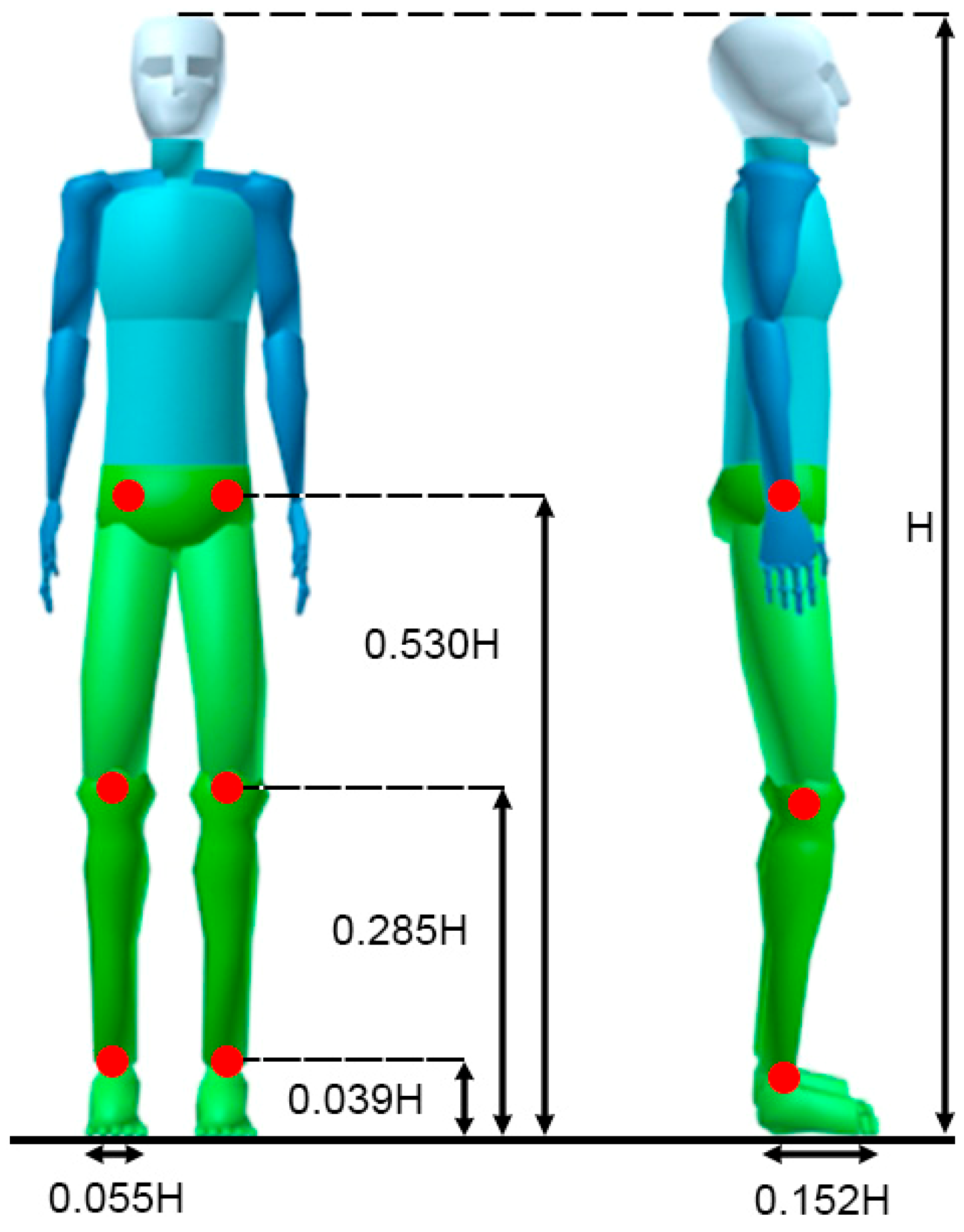
where and are the lower and higher radius of the truncated section, the truncated cone height (all in meters), is the density of the piece, and its mass. As the lower radius is function of itself, the ratio was calculated using direct measurements with a sample of 50 Colombians aged between 18 and 45 years. The length of each section of the leg was calculated using the Drillis and Contini model illustrated in Figure 2. From Equation (3), density () is calculated using the Drillis and Contini equation for average density (human body density), which is shown in Equation (4) [19].
Average density is expressed in terms of the c parameter, which is called the ponderal index or index of corpulence; it is a measure of the contexture calculated as the ratio between mass and body height, where is the size or height of the person in meters and is the mass of the person in kilograms.
Mass and distance to the center of mass are calculated using tabulated data shown in [19]; to simplify calculations, the center of mass distance of each limb segment was considered to be located at 50% of each cone length, resulting in the generalized Hanavan model of the human leg illustrated in Table 1.
Once the Hanavan model is generalized, it is necessary to calculate its kinematics. To do that, the moment of inertia across the “X” axes (see Figure 1) is calculated and is expressed as follows:
This generalized biomechanical model is combined with the double link pendulum model to enhance it and describe the behavior of the exoskeleton coupled to the human leg. According to this, each link of the pendulum is considered as a truncated cone; the kinematics for the proposed model is described in Figure 3.
The displacement of the center of mass is defined as:
where is the angular position of each link, represents each link length. The angular position of the second link is referenced to the first link, so it will be zero if it is aligned with it.
The speed of center of mass is defined as:
The moment of inertia across the center of mass of each segment is defined using Equation (5):
To find the dynamic model of the double pendulum enhanced with the biomechanical model, Lagrange equations of the second kind or Euler-Lagrange equations were used. Those are a reformulation of classical mechanics where the constraints are incorporated directly by the selection of generalized coordinates for the system being studied. Instead of forces, Lagrangian mechanics use the energies in the system, described using the Lagrangian; the nonrelativistic Lagrangian for a system of particles can be defined by:
where T and V are the kinematic energy and potential energy of the system, respectively.
The Euler-Lagrange equation is obtained from Equation (10) and, establishing that, if not all the forces acting on a system are derivable from a potential, those can be written as [20]:
where L contains the potential of conservative forces (Equation (10)), qj represents the generalized coordinates of the system, Qj denotes the generalized forces acting outside the system, and j represents each particle or body analyzed. According to this, external forces acting over the exoskeleton coupled to the leg are considered; those external forces are torque and viscous friction at each joint, and the Euler-Lagrange equation for the system will be:
where represents links 1 and 2 of the pendulum, which denotes the leg and foot. The angle represents the position of each link, is the applied torque, and is the viscous friction coefficient.
To calculate the Lagrangian, it is necessary to define the kinetic and potential energy of the system; kinetic energy is defined as follows [21]:
where is the translational kinetic energy and is the rotational kinetic energy; is the linear speed and is the angular speed of the center of mass, represents bodies mass and is the moment of inertia at the center of mass. Since there are two joints to be considered, the total kinetic energy of the system will be expressed as:
Potential energy is defined as:
so total potential energy for the system will be:
where is the mass of each segment, is the gravity used as , and is the center of mass altitude calculated using the y coordinate of Equations (6) and (7).
Using Matlab-MuPAD, dynamic equations which describe the exoskeleton are calculated by replacing Equations (8) and (9) into Equation (14) to calculate the total kinetic energy of the system; after calculating the kinetic and potential energy, the Lagrangian (10) is calculated and replaced into Equation (12). Once all the parameters are established, Equation (12) is solved and simplified for and , resulting in two nonlinear equations, one for each link describing the dynamic behavior of the proposed system. The resulting dynamic model is:
where:
Those constants are calculated by using Table 1 parameters where is the leg higher radius, the leg lower radius, the foot higher radius, the foot lower radius, the leg length, and the foot length.
This model can be represented as the general form of the Euler-Lagrange equations, such that:
where M is the inertial properties matrix, V the coriolis and centripetal vector, and G the gravity vector of the system. According to the generalized coordinates, the generalized equation for our system is:
where the parameters of Equation (20) are:
2.2. Linear Approximation of the Model
To perform a comparison between the nonlinear model and a linear model suitable to design controllers, the system is linearized.
Since Equations (17) and (18) are second order, it is necessary to transform them into a pair of first-order differential equations, therefore the following variables are introduced:
Those equations are linearized around an equilibrium point based on the Taylor series expansion [22]. Thus, the Equations in (22) can be represented as:
so, the linear approximation of the system will be calculated as follows:
The equilibrium point was selected at the point where the system has lost all its energy; according to the reference settled in Figure 3 it is:
Finally, the linear approximation of the system in state-space is:
where P2 and P3 are the same as in Equations (17) and (18), so:
3. Simulation Results
The aim of the experiments is to validate the developed model by simulation. In this sense, the dynamic models (nonlinear and linear) are implemented to validate the results in the linearization process and the equivalence with the nonlinear model, after which the controllability and observability analysis are performed to the linearized model as a further step to verify the feasibility of control implementation.
3.1. Dynamic Model Simulation
This section describes the developed process to simulate the linear and nonlinear dynamics of the proposed model; for this purpose, Matlab-Simulink was used. Proposed linear and nonlinear models were simulated, calculating its parameters by considering a person with a height of 1.90 m and weight of 90 Kg. Viscous friction at each joint was assumed as and applied torque as , to obtain a lightly damped response of the system. To simulate the exoskeleton, motors and structure weights were added to each link mass; the motors to be used are flat brushless DC motors coupled to a reduction gear capable of generating a maximum torque of 15 Nm. Those motors coupled with the reduction gear box weigh around 0.57 Kg, and the exoskeleton structure was assumed to weigh 0.13 Kg, amounting to a total of 0.7 Kg. These values were added to the second link mass; as the motor acting over the knee at the first link is not going to lift its own weight over the first link, only the structure weight was added.
3.2. Nonlinear Model Simulation
For simulating the nonlinear model, the ordinary differential equation (ODE) system composed by the generalized Euler-Lagrange equation was solved by using its explicit form:
where M is the inertial properties matrix, V the coriolis and centripetal vector, and G the gravity vector of the system. According to the generalized coordinates, the generalized equation for our system is:
where each matrix parameter is shown in Equation (21). After calculations with selected personal characteristics, they are defined as:
Once the system of ordinary differential equations (ODEs) is defined, it is necessary to reduce it from two second-order equations to four first-order equations; this is done by applying the same process employed for linearizing the model. This time, for the nonlinear functions described by Equation (27), the following variables must be introduced:
where corresponds to each expression given by solving Equation (27):
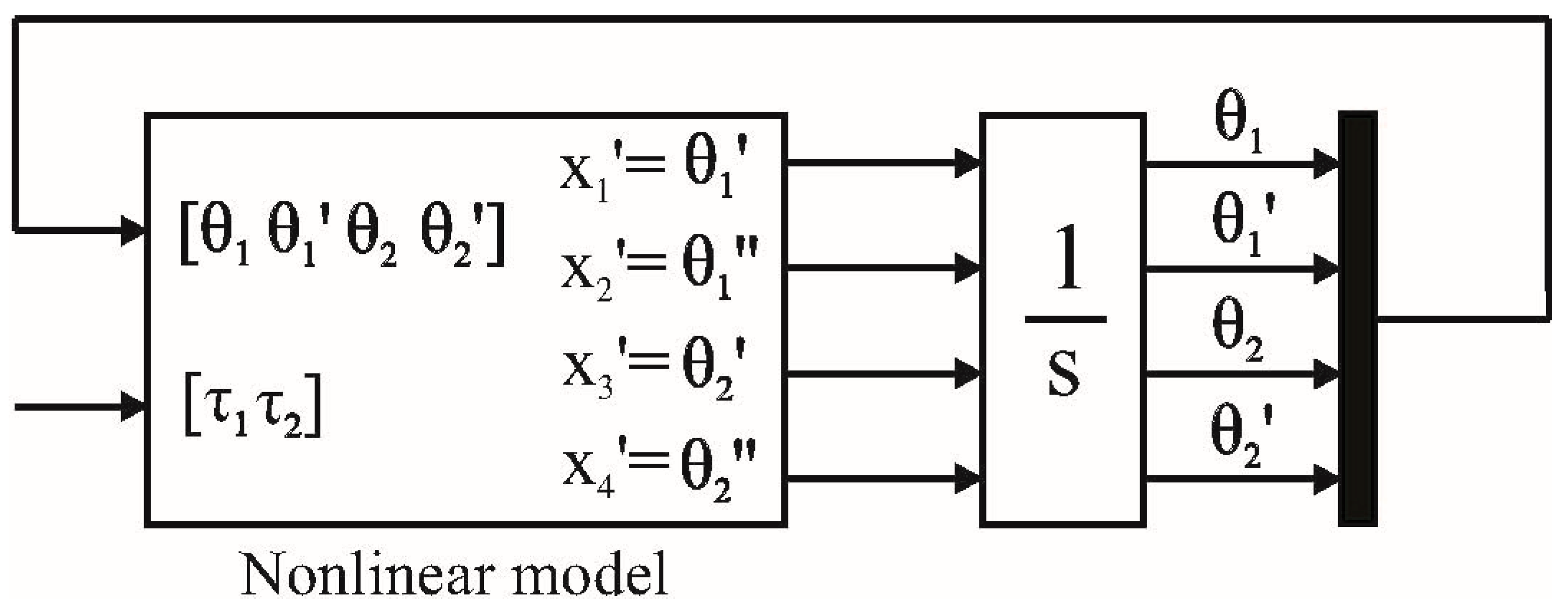
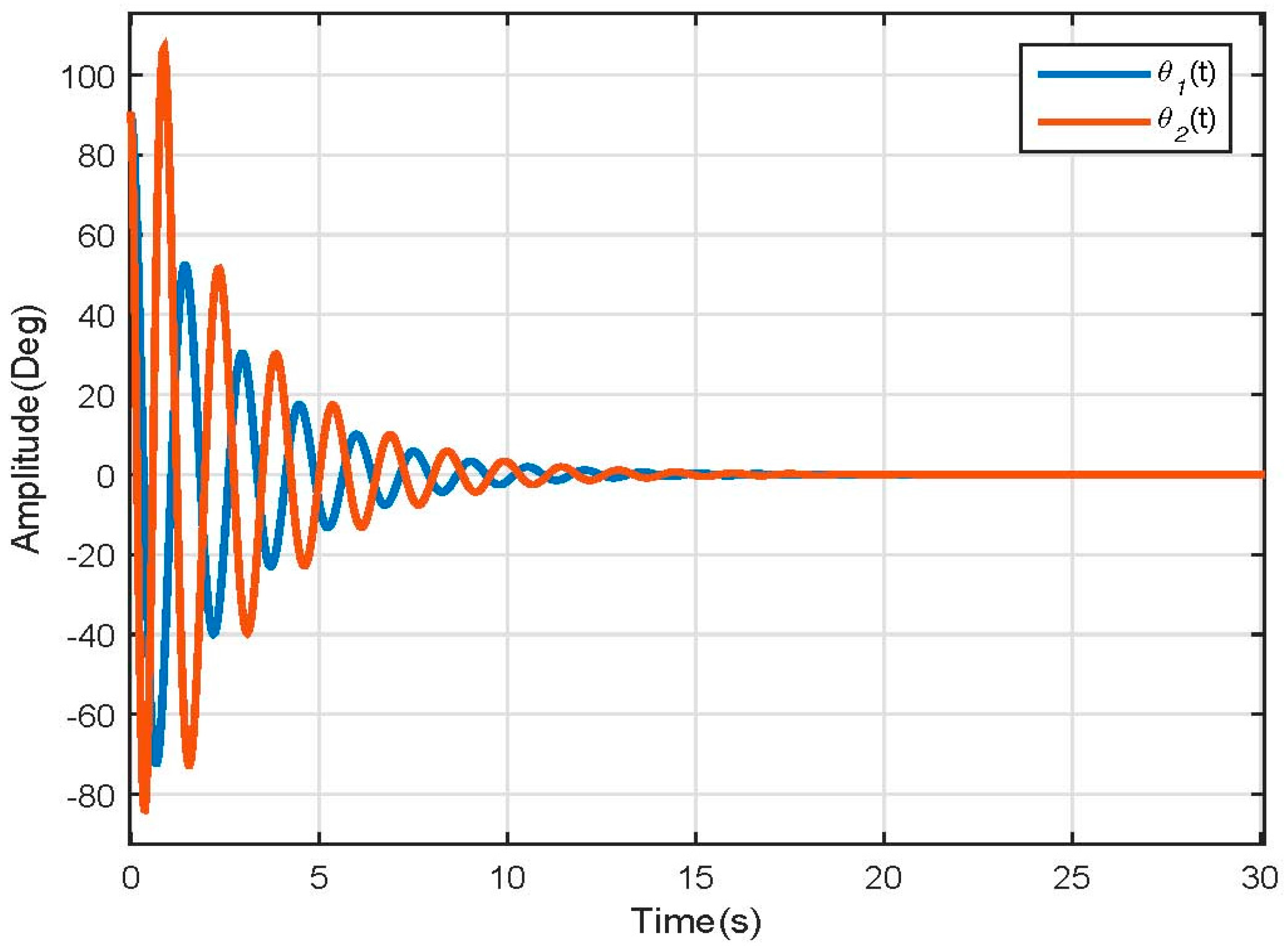
Simulink “ode15s” solver was selected to solve this ODE system, and as a nonlinear model reference uses horizontal axes as 0° degrees and the gravity vector (G(q)) is used, no initial conditions were needed. The simulation block diagram is illustrated in Figure 4 and the dynamic behavior of the model is shown in Figure 5.
The model behavior was as expected; the first link falls and moves describing a damped sine wave, which loses energy due to friction causing it to stabilize in −90°, and the second link movement is induced by the movement of the first link—as its angle is referenced to the first link, it stabilizes on line with it, which is why it reaches 0°. The model speed response is illustrated in Figure 6.
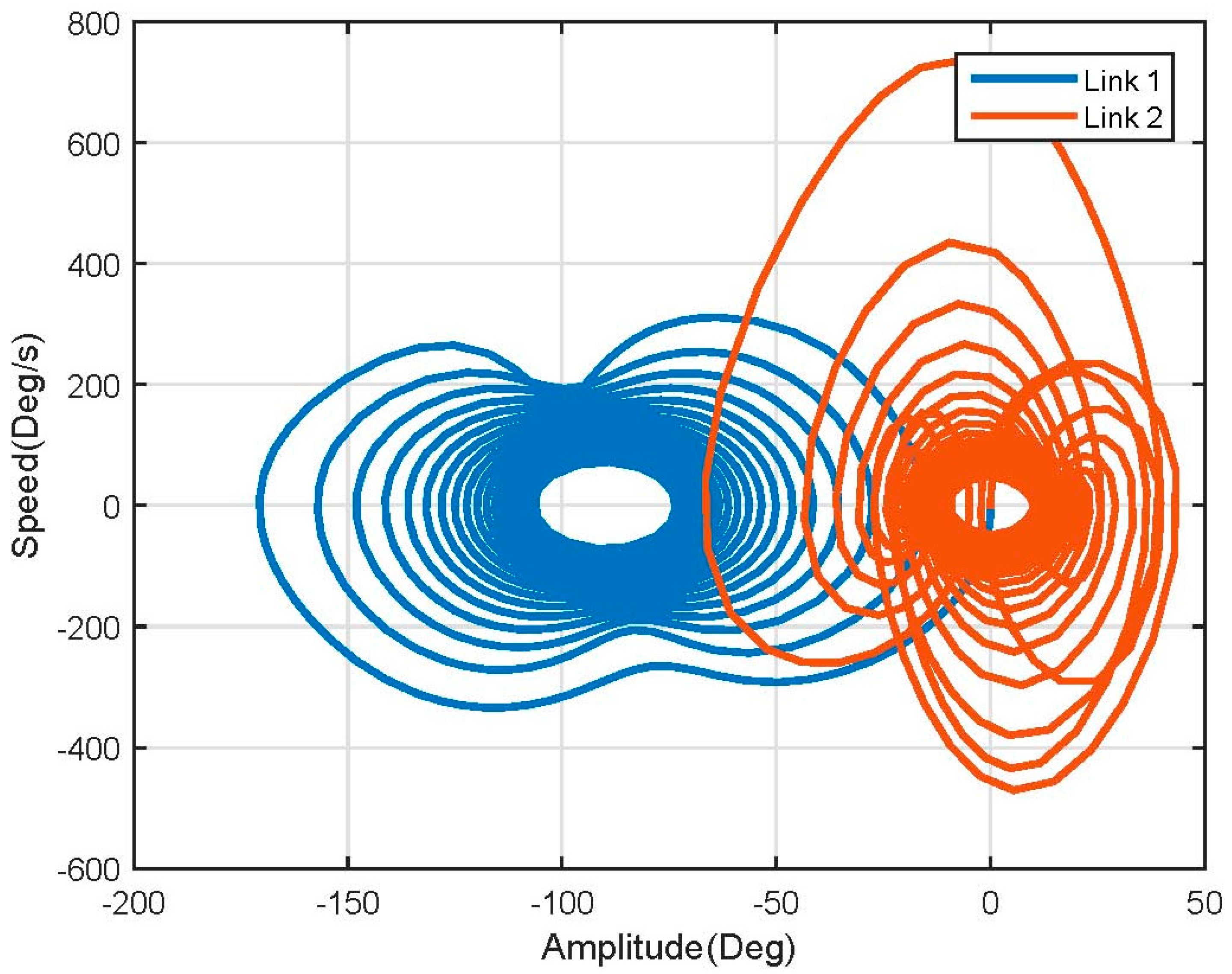
Using Figure 7, it is easy to see that the nonlinear system has two equilibrium points at (90, 0) and (0, 0); this is what allowed us to define and apply the linearization method mentioned before.
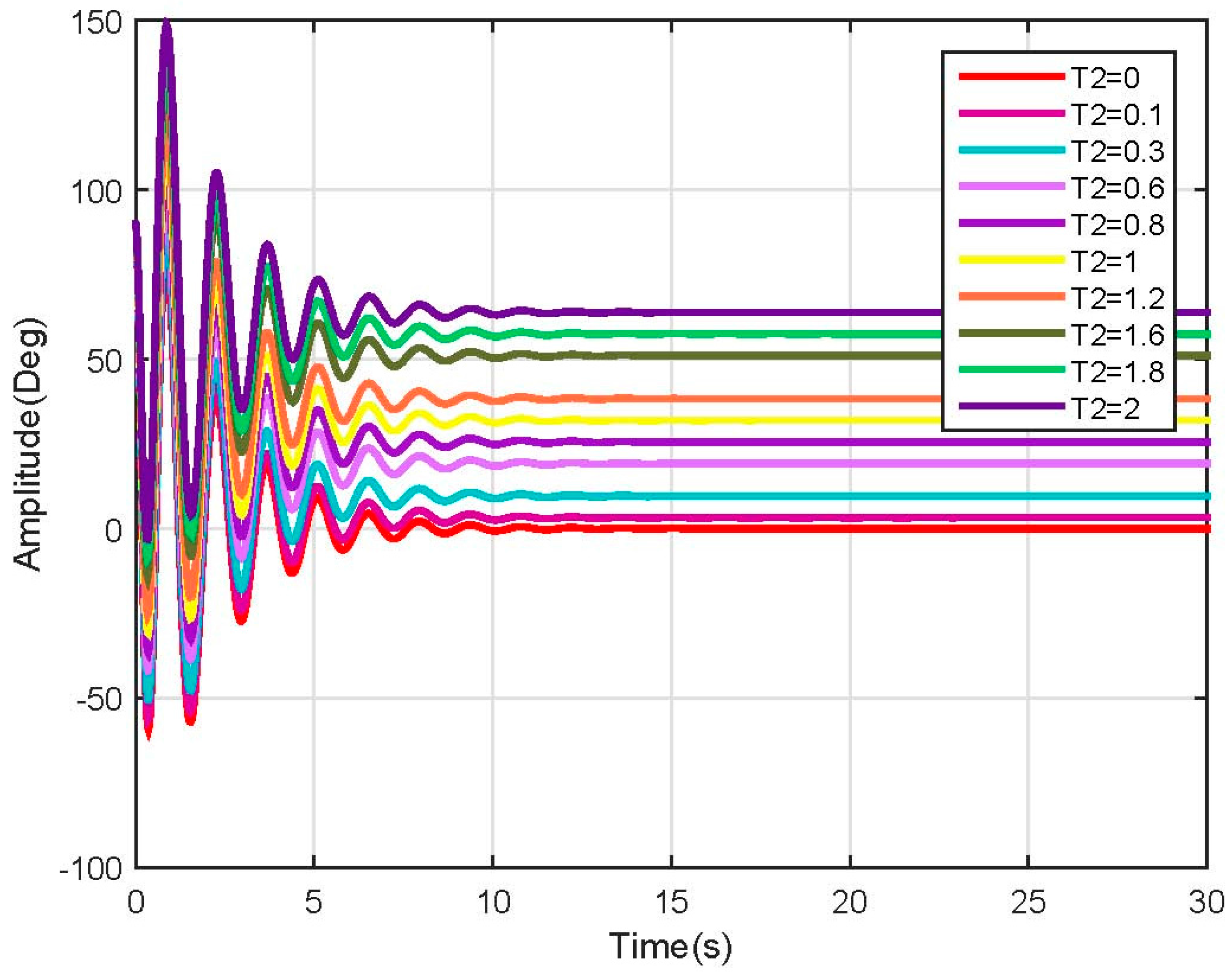
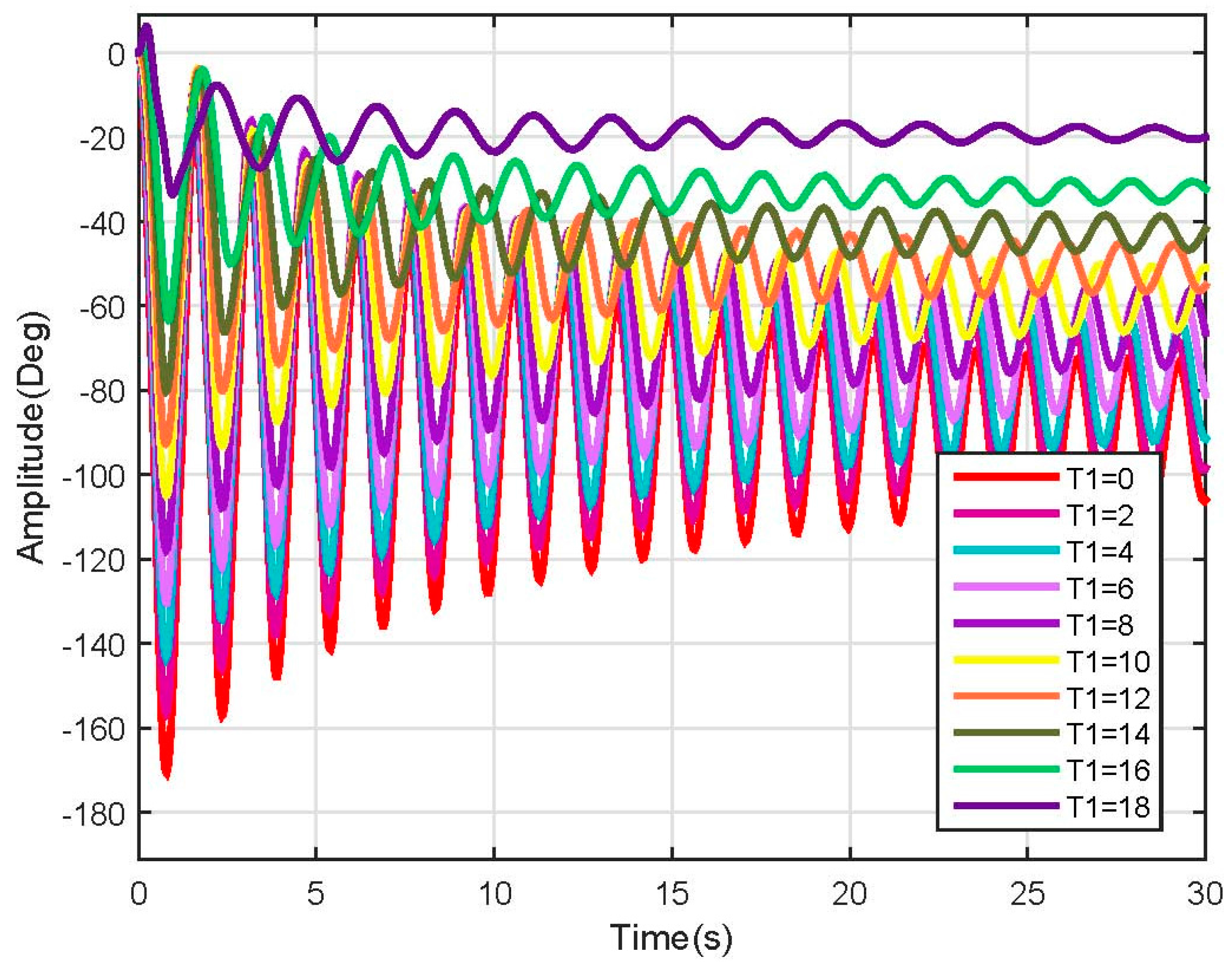
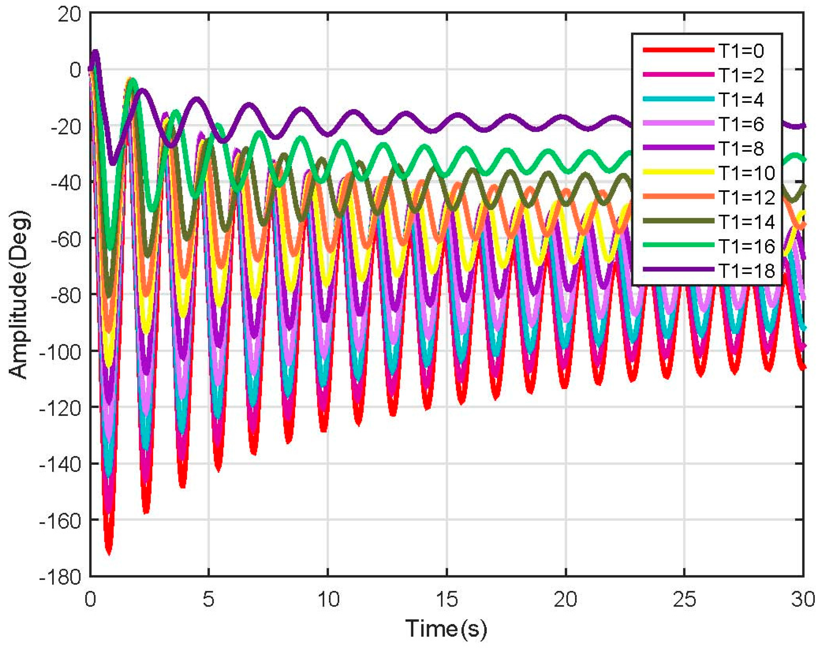
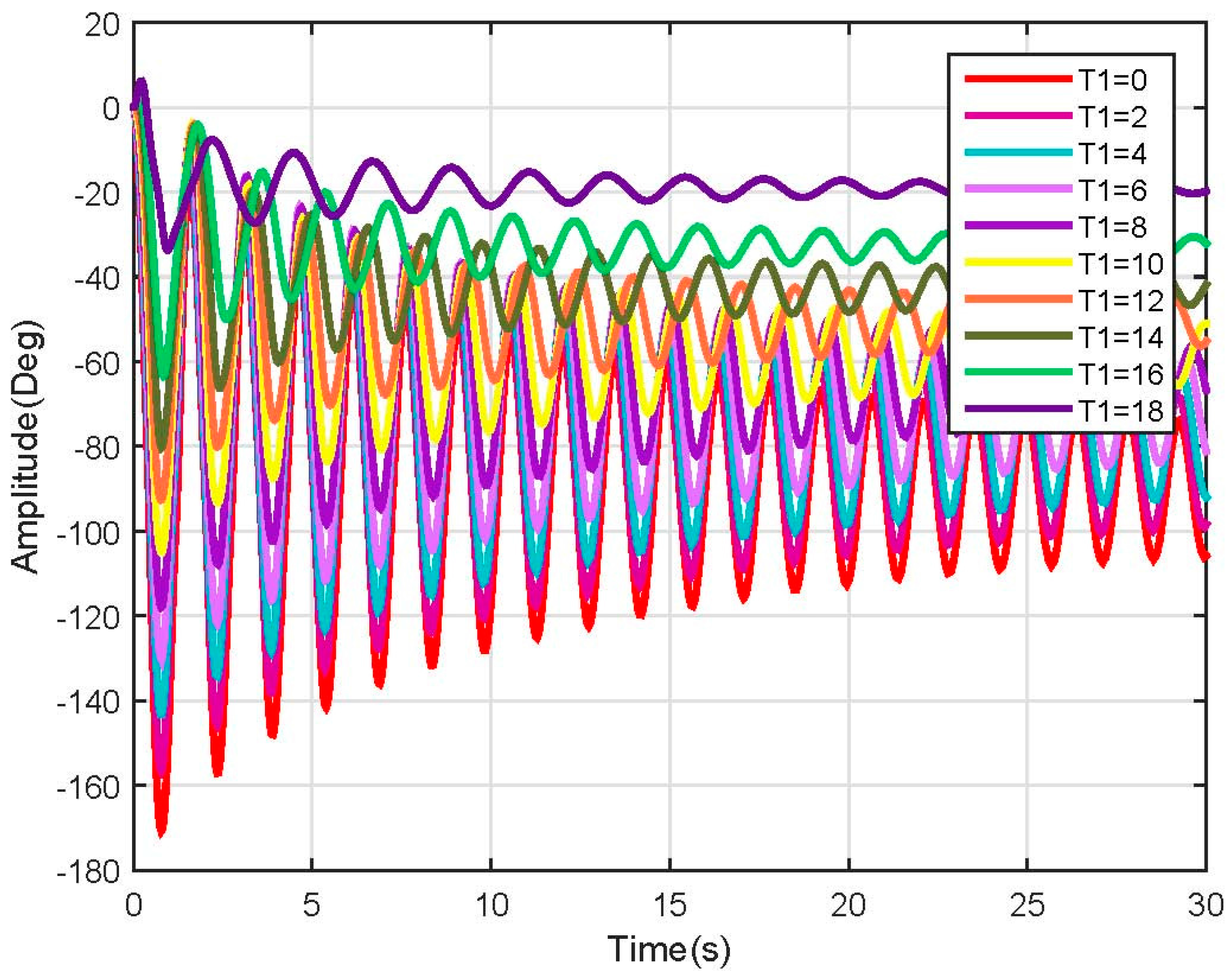
As the purpose of the proposed model is to be controlled, to check if the input variable of the system affects its stabilizing point for a possible position control, different torque values were applied to each link. Tests were done by applying torques to the first link in between 0 and 18 Nm while the applied torque to the second link was 0 Nm; for the second link, due to its low mass, torques between 0 and 2.5 Nm were applied while the applied torque to the first link was 0 Nm. Results are shown in Figure 8 and Figure 9.
For the first link, the test torque vector is defined as Equation (31); each element in the vector corresponds to an applied torque at each joint:
After applying this vector to the system, is clear that this input modifies the model steady state value, which is as expected for control purposes. Furthermore, it also affects the oscillation behavior of the system, making it slower and decreasing its amplitude (see Figure 8).
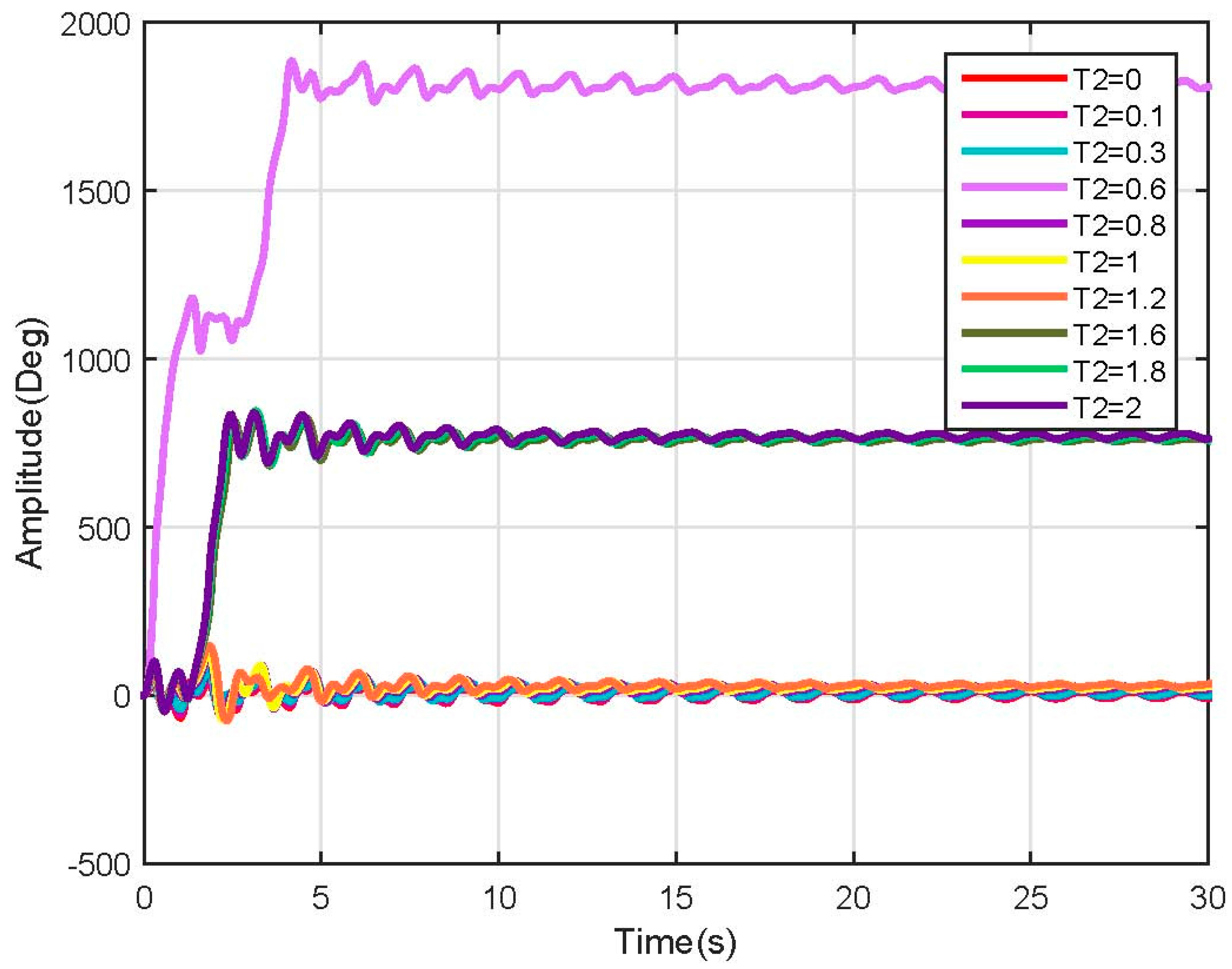
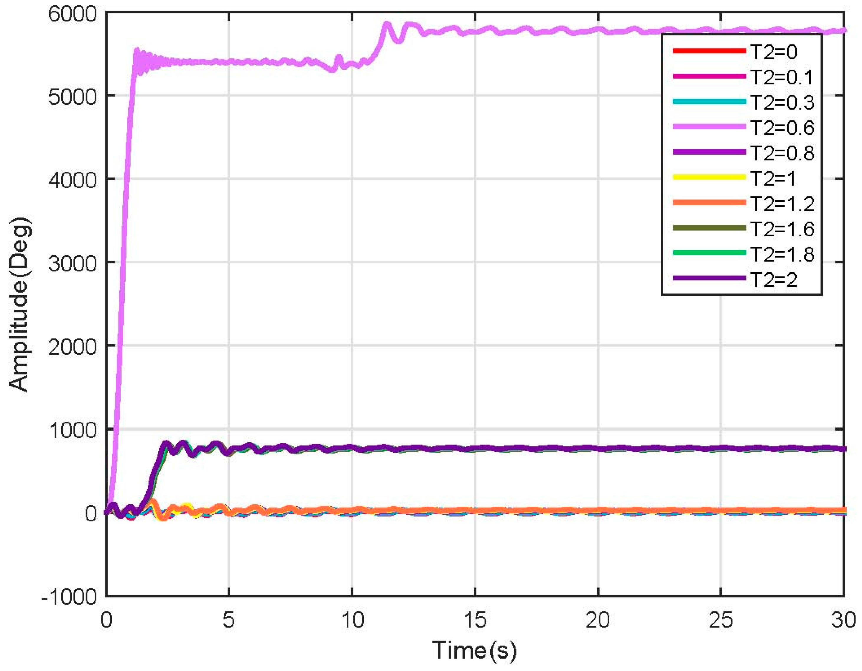
For the second link, the test torque vector is defined as:
Making some tests and applying different torque values to the second link, some instability points were encountered for input (). The model response for the second link is shown in Figure 9, due to its nonlinearities, it is possible to observe that different answers are obtained with different behaviors, but after 1.2 Nm the system becomes completely unstable (see Figure 9).
To check the behavior of the model when user characteristics vary, several tests were performed following the simulation scheme used before; a few of those tests are shown below. For this purpose, we refer to them as test 2 and test 3; test 2 was conducted by simulating a person of 65 Kg, 1.70 m tall, and test 3 simulated a person of 50 Kg, 1.50 m tall (See Figure 10, Figure 11, Figure 12 and Figure 13).
Test 2:
Figure 10.
Link 1, test 2 position response (Non-linear).

Figure 11.
Link 2, test 2 position response (Non-linear).

Test 3:
Figure 12.
Link 1, test 3 position response (Non-linear).

Figure 13.
Link 2, test 3 position response (Non-linear).

In the above-mentioned tests, many more nonlinearities were encountered when varying the user characteristics, which could be mitigated by using robust nonlinear controllers. Besides the nonlinearities, the system behavior was as expected and followed the results shown before.
3.3. Linear Model Simulation
Calculating all parameters and applying them to Equation (25), it is possible to obtain the following state-space representation of the linear approximation of the model:
Matlab-Simulink was used to obtain the system time response; due to the linear approximation method used, made around the equilibrium point (Equation 24), the system reference changed. Thus, the system 0° degrees are located at the negative vertical axes so initial conditions were needed, which were taken as . Results are shown in Figure 14.
The linear model differs from the nonlinear model response, but behaves as expected following the dynamics of a double pendulum stabilizing at 0° degrees. This because the linear model is merely an approximation made to work with the nonlinearities present in the original model. This model is affected in a higher way for the friction factor than the dynamical one; therefore, it loses energy faster and reaches the steady state faster. The model speed response is illustrated in Figure 15.
With this linear approximation, the phase diagram softens and converges into the steady state value more smoothly than the nonlinear one (see Figure 16).
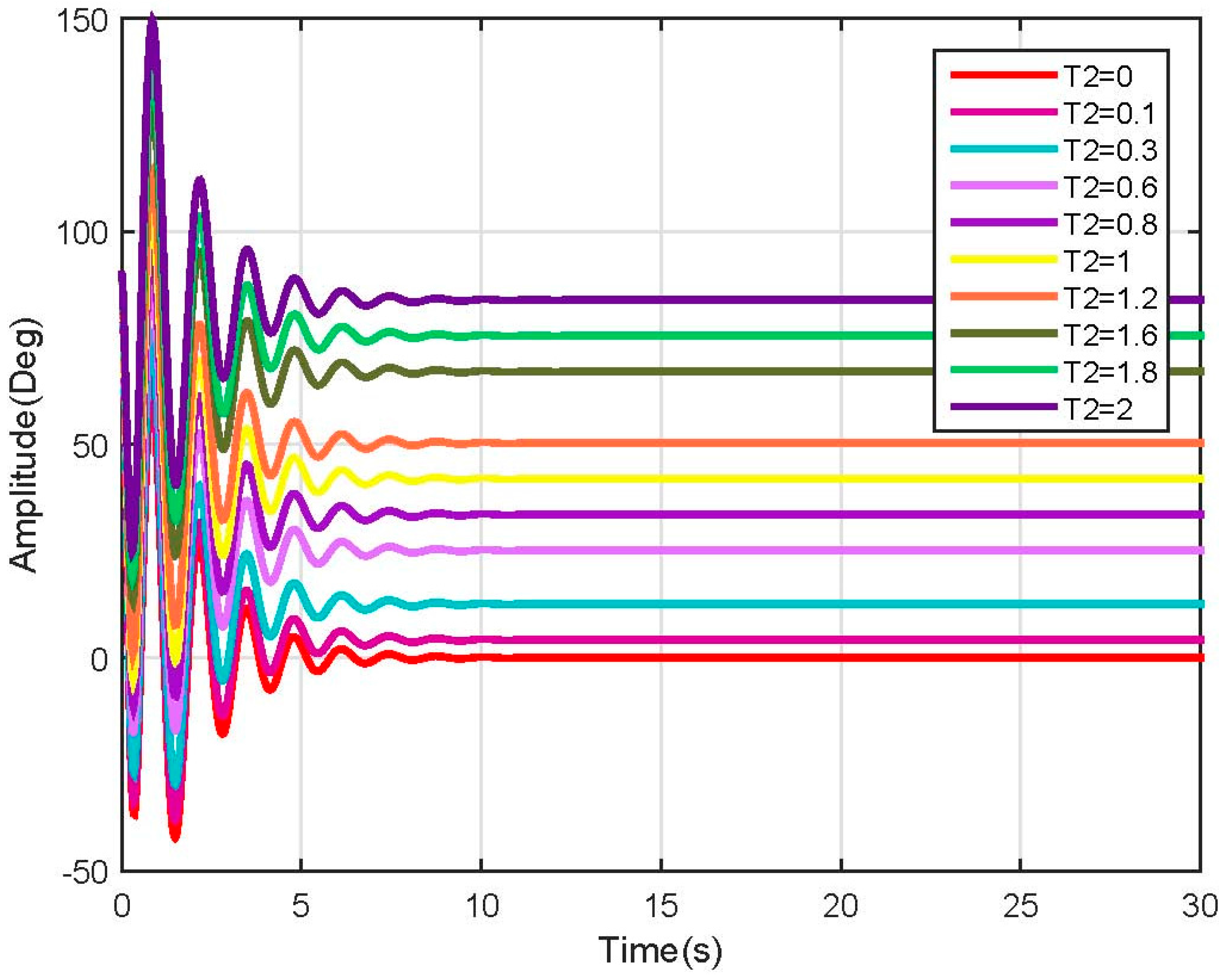
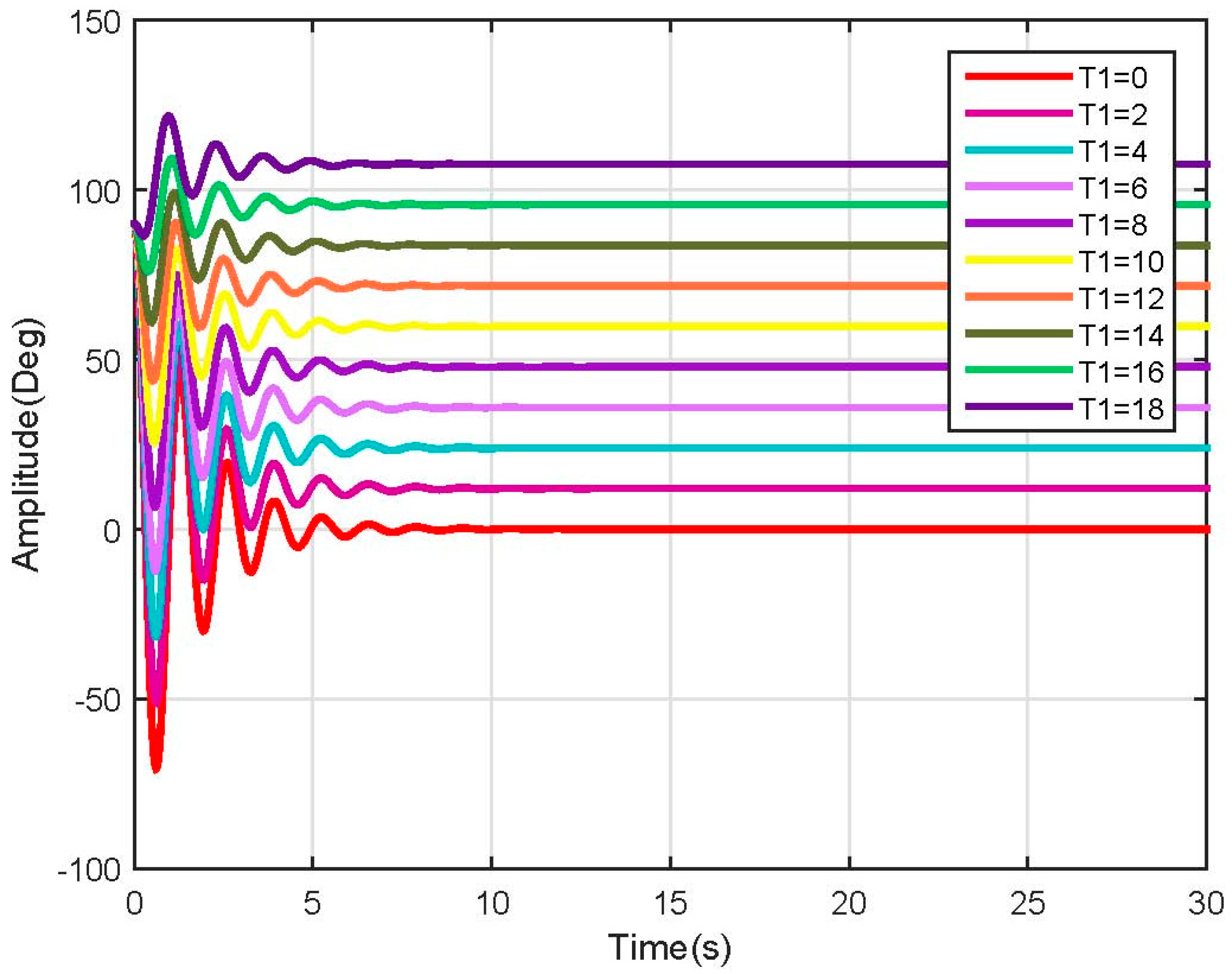
To check if the input variable of the system affects its stabilizing point, the same vectors of Equations (31) and (32) were applied to the linear model, the results of which are shown in Figure 17 and Figure 18.
For both links, each input produces a significant change in the steady state of the model. It also reveals that the nonlinearity which produced the uncontrolled increase in the response of the system was eliminated, making the system proper for control design and tuning.
Test 2:
Figure 19.
Link 1, test 2 position response (Linear).
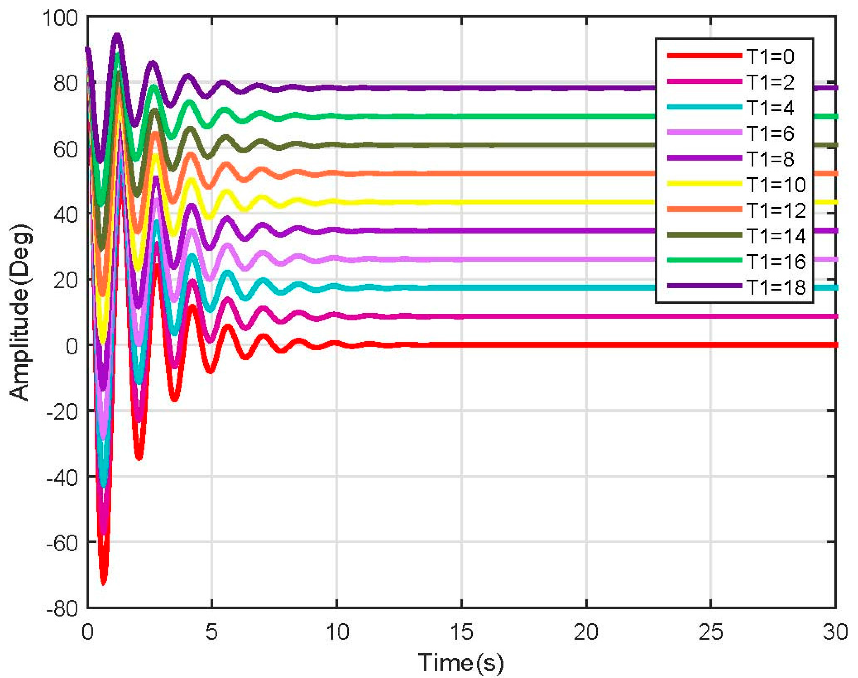
Figure 20.
Link 2, test 2 position response (Linear).
Test 3:
Figure 21.
Link 1, test 3 position response (Linear).

Figure 22.
Link 2, test 3 position response (Linear).
As expected, the linearized model behavior stabilizes at a different rate according to the mass and length of each segment of the leg. This speed change requires a robust speed control in order to avoid injuring a person with different characteristics when using the same device; it also could be configurable to enhance the therapy.
4. Observability and Controllability Analysis
The linear model is planned to be used to design and tune linear control strategies, which is why it must be analyzed to ensure that it is controllable and/or observable. Defining the controllability matrix (Co) and observability matrix (O) as:
where n is the range of A matrix. Using the linear state-space of Equation (33), which is in the form:
it is easy to define that n = 4, so our analysis will be defined as:
replacing the matrices of Equation (33) into Equations (34) and (35) will result in a controllability matrix of dimensions (4 × 8) and an observability matrix of dimensions (8 × 4), as the model is a multi-input multi-output (MIMO) system with two inputs and two outputs. To obtain the controllability matrix for each input-output pair, it is necessary to take columns (1–7) of Co to build the controllability matrix for the first pair () and to take columns (2–8) to build the controllability matrix for the second pair (); in the case of observability, is the same process but selecting rows. The controllability and observability matrices will look like:
Nonsingular matrices indicate that the system is fully observable and controllable.
5. Exoskeleton Design Proposal
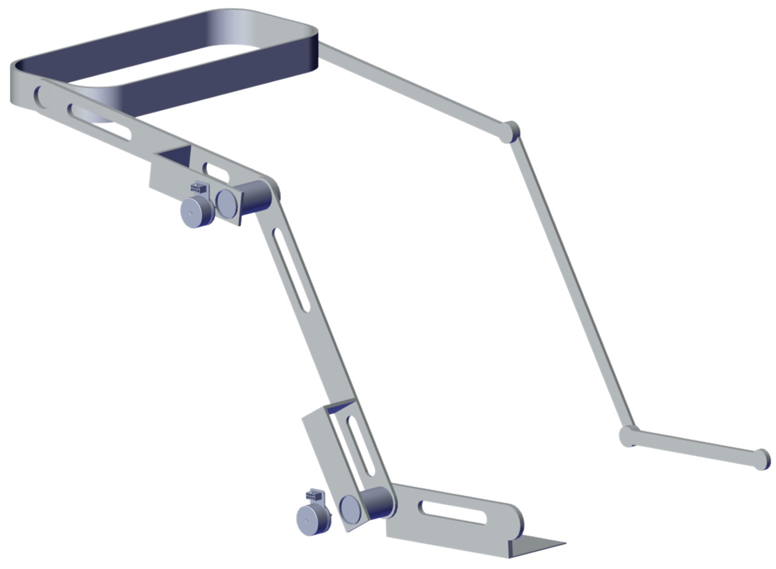
The model previously described is oriented to describe a simple exoskeleton with 2 DOF. Figure 23 and Figure 24 show the general idea for the implementation; the exoskeleton consists of active and passive elements which are attached to the legs in a non-invasive way. The main idea is that the device can be wearable and adapted to the features of individual patients.
The structure is intended to work as Master-Slave, where one leg controls the other one. This enables the user to use the non-injured leg to perform rehabilitation exercises that can be replicated in the injured one. The employed actuators are planned to be brushless DC motors coupled to a reduction gear (see Figure 25 and Figure 26).
6. Conclusions
The contribution of this paper focuses on extending the exoskeleton line of research by proposing a new way of modeling such that the followed objective is to develop a dynamic model using a combination of different models which mathematically describe the human body. The proposed model is a combination of three models, which, when united, can describe the physical behavior of the exoskeleton frame coupled to the human leg. This model has the advantage that it can be calculated for any kind of person given their its mass and height, converting it into a flexible alternative for calculating the exoskeleton dynamics very quickly and adapting them easily for a child’s or young adult’s body. As a secondary goal, the paper focuses on showing that the model can be controlled in different ways to satisfy the different characteristics of each possible rehabilitation therapy for which the exoskeleton could be used. As the resulting model is a highly nonlinear model, it was linearized and tested using simulation environments to ensure that it works as expected and its able to design and test control strategies. The linear representation results were fully controllable and observable, which fulfills the secondary objective proposed. Since this work was focused in the mathematical model description, and its validation was performed by software simulation, it is necessary to perform a validation with the physical device. As future work, tests with the physical device will be conducted and tests with human patients will then be considered so as to define a medical protocol to evaluate the device under the supervision of physical therapists. This model is also planned to be extended to three links, to be used to describe all leg movements in the sagittal plane. Also, control strategies including force feedback and/or joint virtual torque control with gravity compensation will be tested with the real equipment.
Author Contributions
C.V., D.T. and M. Anaya conceived and designed the experiments; C.V. and D. T. proposed the definition of the generalized model; C. V., D.T. and M.A. wrote the paper.
Conflicts of Interest
The authors declare no conflict of interest.
References
- Cao, H.; Ling, Z.; Zhu, J.; Wang, Y.; Wang, W. Design Frame of a Leg Exoskeleton for Load-Carrying Augmentation. In Proceedings of the 2009 IEEE International Conference on Robotics and Biomimetics (ROBIO), Guilin, China, 19–23 December 2009. [Google Scholar]
- Jin, X.; Agrawal, S.K. Exploring Laparoscopic Surgery Training with Cable-Driven ARm EXoskeleton (CAREX-M). In Proceedings of the 2015 IEEE International Conference on Rehabilitation Robotics (ICORR), Singapore, 11–14 August 2015. [Google Scholar]
- Misgeld, B.; Schauer, T.; Simanski, O.; Hessinger, M.; Müller, R.; Werthschützky, R.; Pott, P.P. Tool Position Control of an Upper Limb Exoskeleton for Robot-Assisted Surgery. IFAC-PapersOnLine 2015, 48, 195–200. [Google Scholar]
- Banala, S.K.; Agrawal, S.K.; Scholz, J.P. Active Leg Exoskeleton (ALEX) for Gait Rehabilitation of Motor-Impaired Patients. In Proceedings of the 2007 IEEE 10th International Conference on Rehabilitation Robotics (ICORR 2007), Noordwijk, The Netherlands, 13–15 June 2007. [Google Scholar]
- Crema, A.; Mancuso, M.; Frisoli, A.; Salsedo, F.; Raschella, F.; Micera, S. A Hybrid NMES-Exoskeleton for Real Objects Interaction. In Proceedings of the 2015 7th International IEEE/EMBS Conference on Neural Engineering (NER), Montpellier, France, 22–24 April 2015. [Google Scholar]
- Kim, H.; Miller, L.M.; Fedulow, I.; Simkins, M.; Abrams, G.M.; Byl, N.; Rosen, J. Kinematic Data Analysis for Post-Stroke Patients Following Bilateral versus Unilateral Rehabilitation with an Upper Limb Wearable Robotic System. IEEE Trans. Neural Syst. Rehabil. Eng. 2013, 21, 153–164. [Google Scholar] [CrossRef] [PubMed]
- Lee, H.; Kim, J.; Kim, T. A Robot Teaching Framework for a Redundant Dual Arm Manipulator with Teleoperation from Exoskeleton Motion Data. In Proceedings of the 2014 IEEE-RAS International Conference on Humanoid Robots, Madrid, Spain, 18–20 November 2014. [Google Scholar]
- Safavi, S.; Ghafari, A.S.; Meghdari, A. Design of an Optimum Torque Actuator for Augmenting Lower Extremity Exoskeletons in Biomechanical Framework. In Proceedings of the 2011 IEEE International Conference on Robotics and Biomimetics (ROBIO), Karon Beach, Phuket, Thailand, 7–11 December 2011. [Google Scholar]
- Surachai, P. Design and simulation of leg-exoskeleton suit for rehabilitation. Glob. J. Med. Res. 2012, 12, 1–8. [Google Scholar]
- Pan, M.; Zhang, D.; Gao, Z. Novel Design of a Three Degrees of Freedom Hip Exoskeleton Based on Biomimetic Parallel Structure. In Proceedings of the 2011 IEEE International Conference on Computer Science and Automation Engineering (CSAE), Shanghai, China, 10–12 June 2011. [Google Scholar]
- Velandia, C.; Celedón, H.; Tibaduiza, D.A.; Torres-Pinzón, C.; Vitola, J. Design and Control of an Exoskeleton in Rehabilitation Tasks for Lower Limb. In Proceedings of the 2016 XXI Symposium on Signal Processing, Images and Artificial Vision (STSIVA), Bucaramanga, Colombia, 31 August–2 September 2016. [Google Scholar]
- Ferrati, F.; Bortoletto, R.; Pagello, E. Virtual Modelling of a Real Exoskeleton Constrained to a Human Musculoskeletal Model. In Proceedings of the Second International Conference Biomimetic and Biohybrid Systems, Living Machines 2013, London, UK, 29 July–2 August 2013; Springer: Berlin/Heidelberg, Germany, 2013. [Google Scholar]
- Lu, R.; Li, Z.; Su, C.-Y.; Xue, A. Development and Learning Control of a Human limb with a Rehabilitation Exoskeleton. IEEE Trans. Ind. Electron. 2014, 61, 3776–3785. [Google Scholar] [CrossRef]
- Xiuxia, Y.; Yi, Z.; Zhicai, X.; Zhiyong, Y. Total Cource Locomotion Control of Assist Walking Exoskeleton Leg. In Proceedings of the 2011 30th Chinese Control Conference (CCC), Yantai, China, 22–24 July 2011. [Google Scholar]
- Singla, A.; Dhand, S.; Virk, G.S. Mathematical modelling of a hand crank generator for powering lower-limb exoskeletons. Pespect. Sci. 2016, 8, 561–563. [Google Scholar] [CrossRef]
- Cardenas, C.C.V. Modelado, Control Y Monitoreo de un Exoesqueleto Pistir Procesos de Rehabilitacion en Miembro Inferior; Universidad Santo Tomás: Bogotá, Colombia, 2016. [Google Scholar]
- Hanavan, E.P., Jr. A mathematical model of the human body. AMRL TR 1964, 1–149. [Google Scholar]
- Drillis, R.; Contini, C. Body Segment Parameters Artificial Limbs; National Academy of Sciences: Washington, DC, USA, 1964; Volume 8, pp. 44–67. [Google Scholar]
- Winter, D.A. Biomechanics and Motor Control of Human Movement, 4th ed.; John Wiley and Sons, Inc.: Hoboken, NJ, USA, 2009. [Google Scholar]
- Goldstein, H.; Poole, C.; Safko, J. Classical Mechanics, 3rd ed.; Addison Wesley: Indianapolis, IN, USA, 2001. [Google Scholar]
- Young, H.D.; Freedman, R.A. Fisica Universitaria, 12th ed.; Pearson Educación: México City, México, 2009. [Google Scholar]
- Ogata, K. Ingenieria de Control Moderna; Pearson Educación: New York, NY, USA, 2009. [Google Scholar]
Figure 1.
Truncated cone kinematic analysis.
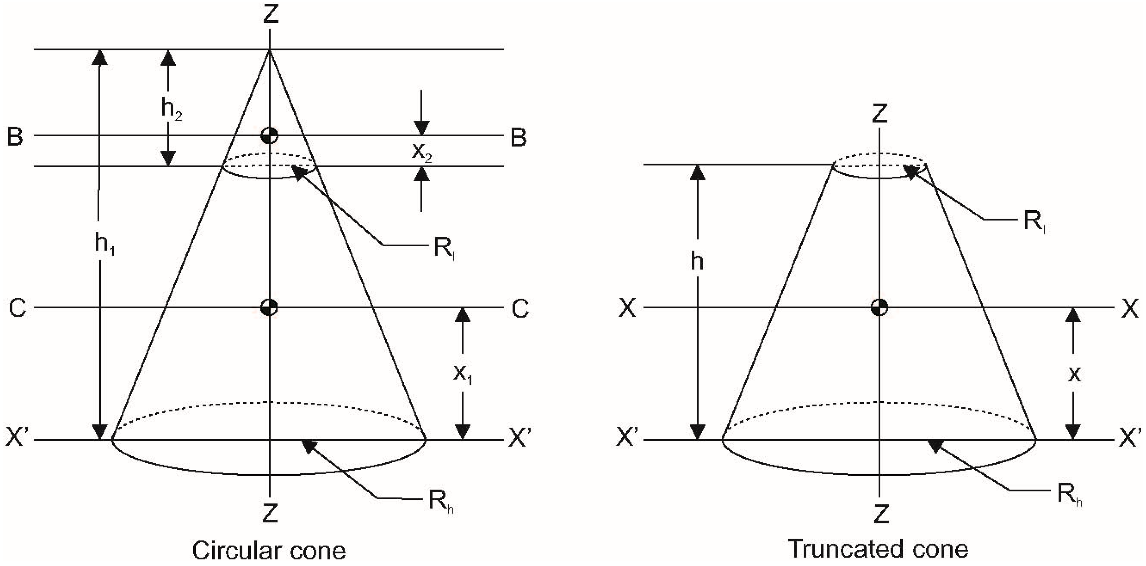
Figure 2.
Body segment length according to D&C model.

Figure 3.
Leg double pendulum representation reference frame.
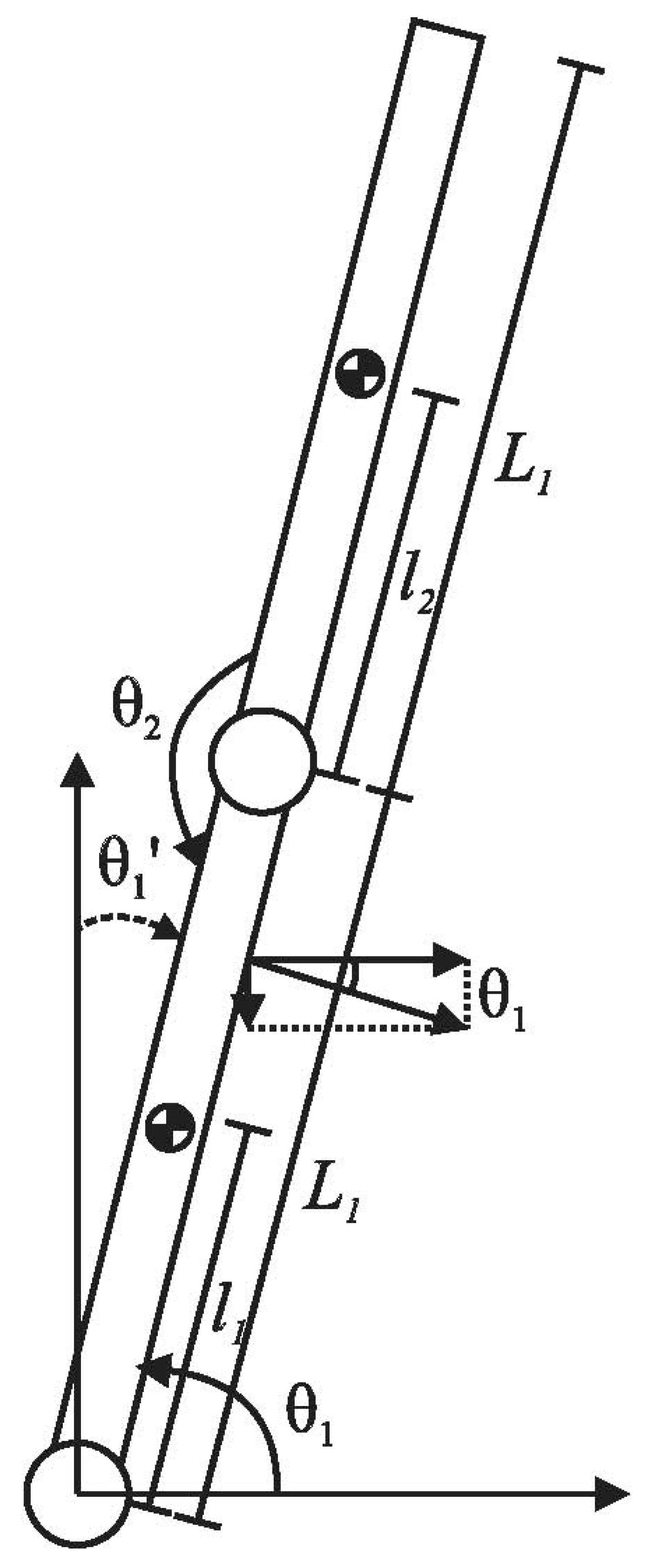
Figure 4.
Non-linear model simulation scheme.

Figure 5.
Non-linear model positions response.
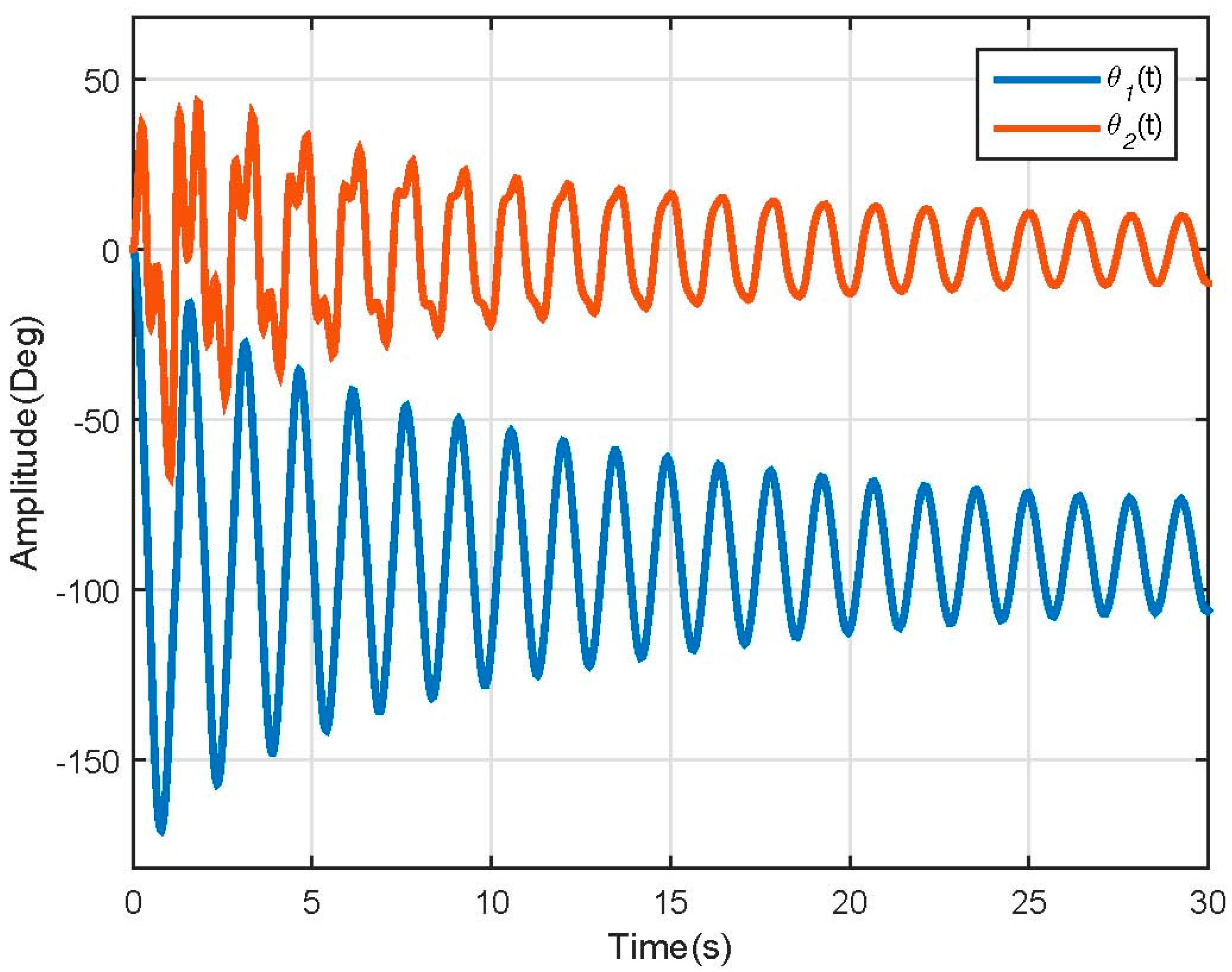
Figure 6.
Non-linear model speed response.
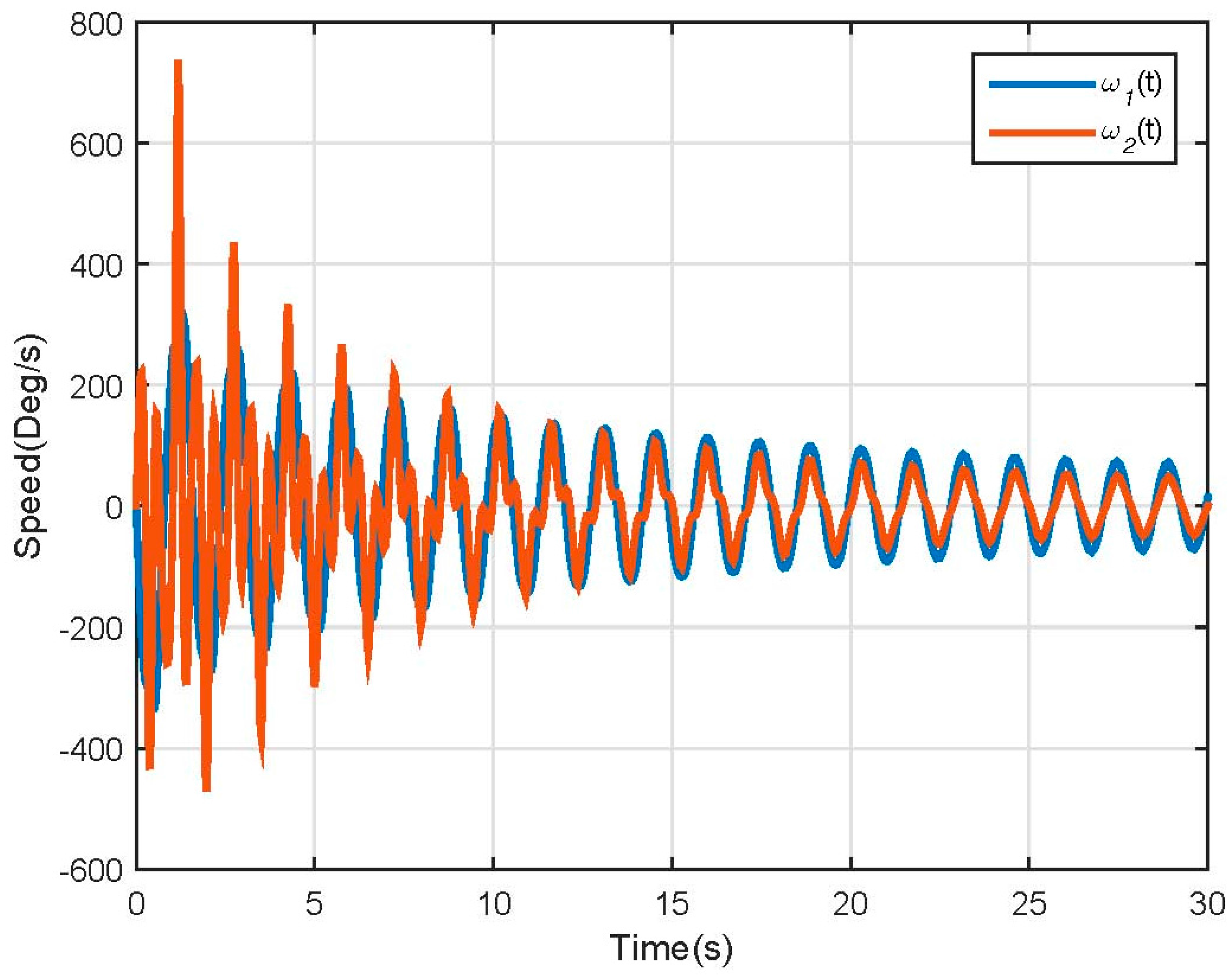
Figure 7.
Non-linear model phase plane.

Figure 8.
Link 1 position response (Non-linear).

Figure 9.
Link 2 position response (Non-linear).
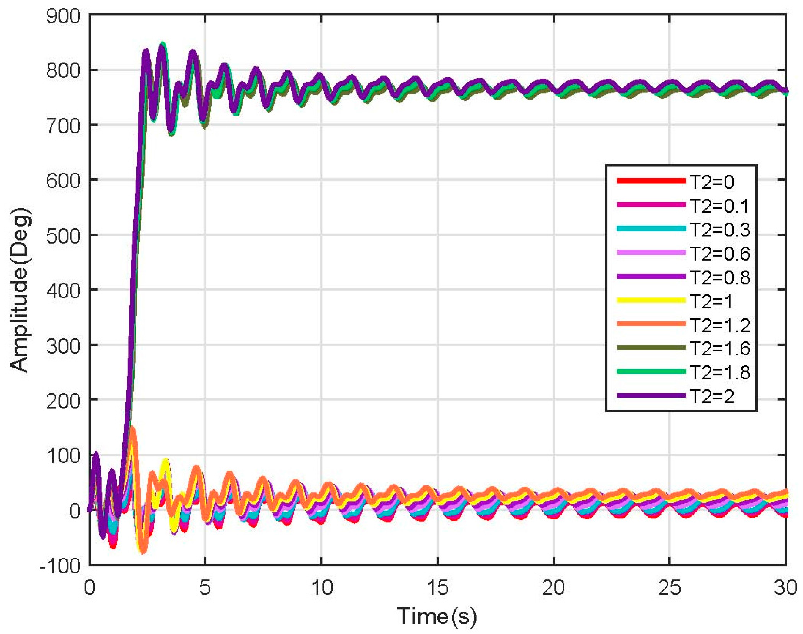
Figure 14.
Linear Model Position response.

Figure 15.
Linear Model Speed response.
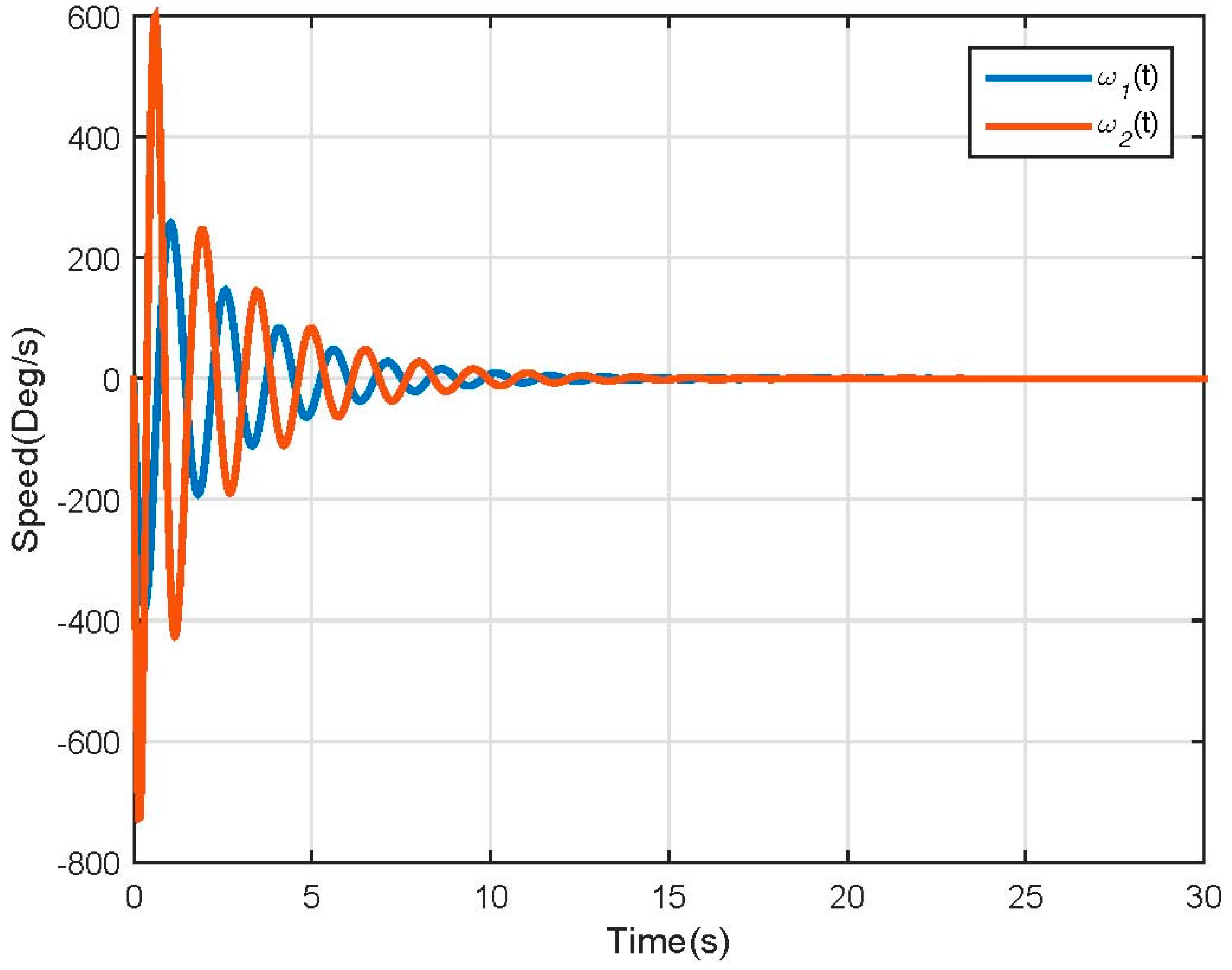
Figure 16.
Linear model phase plane.
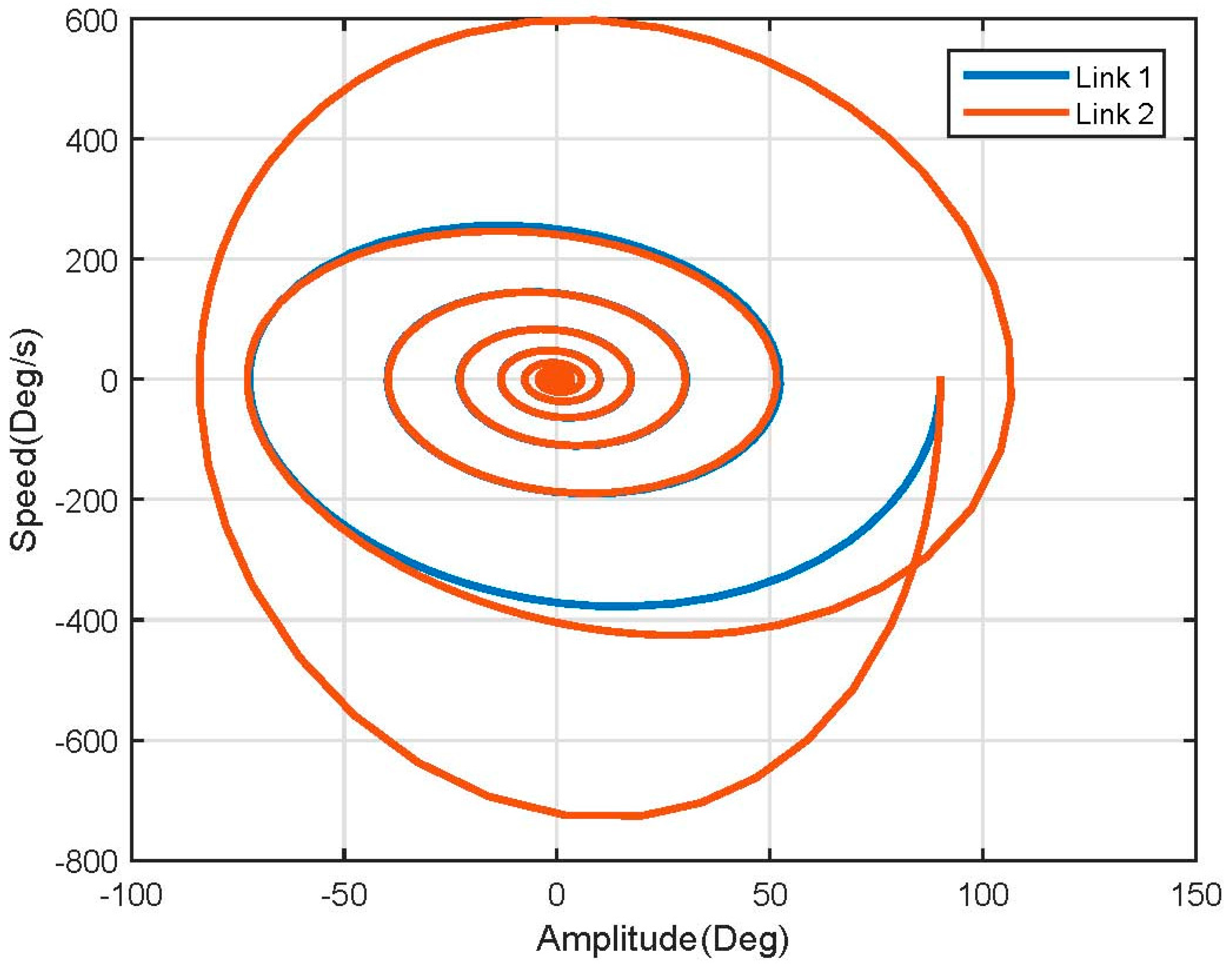
Figure 17.
Link 1 position response (Linear).
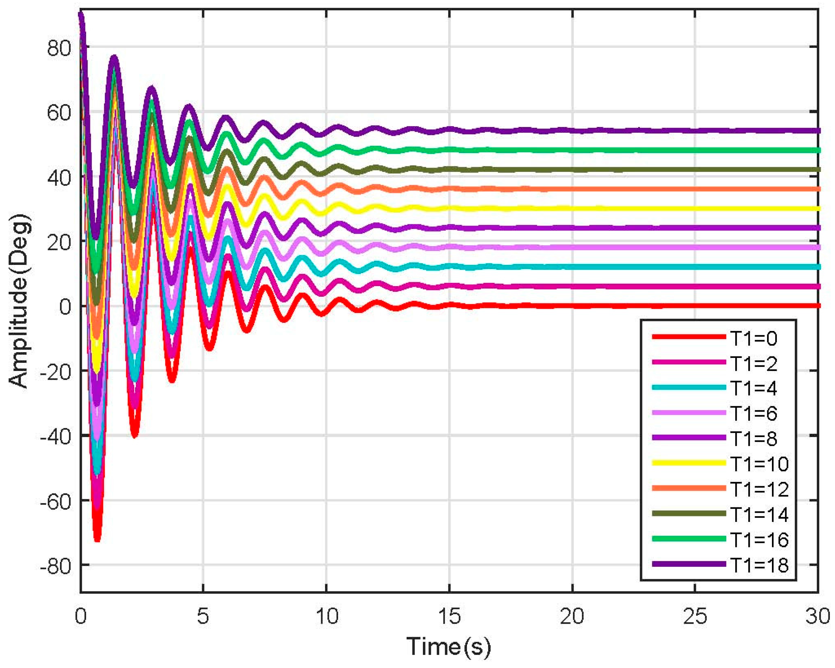
Figure 18.
Link 2 position response (Linear).
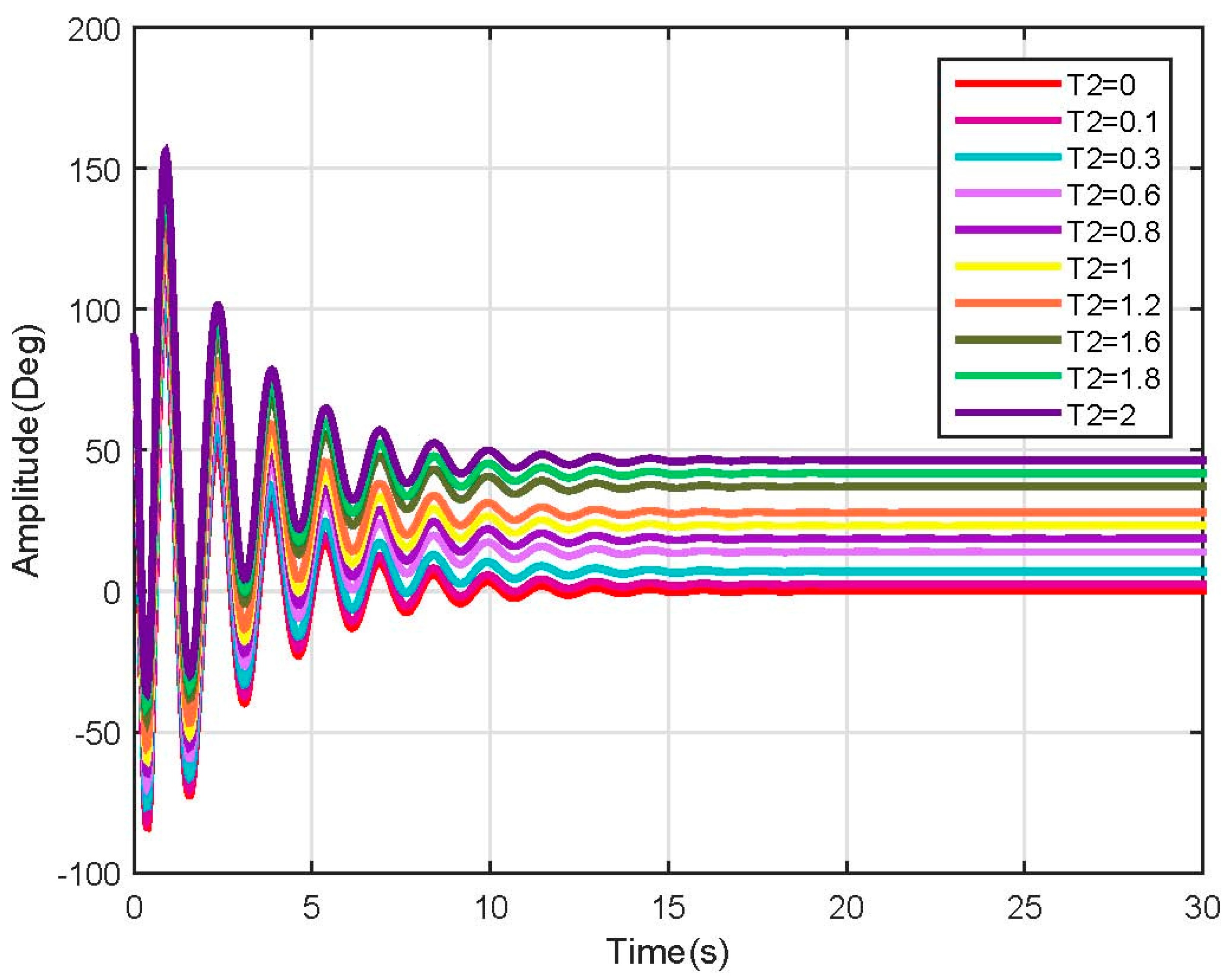
Figure 23.
Exoskeleton proposed design (Right view).

Figure 24.
Exoskeleton design proposal (Left view).
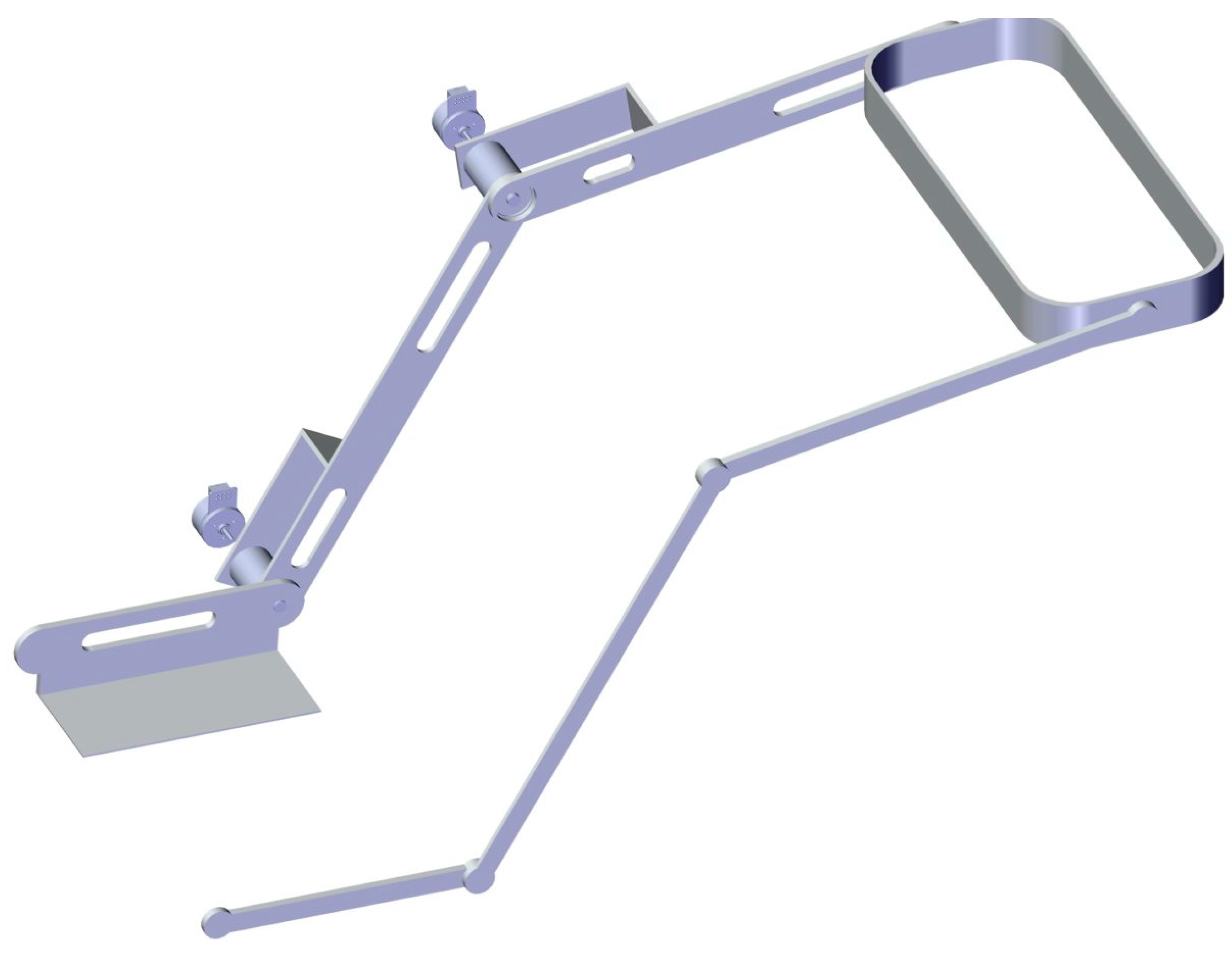
Figure 25.
Motor coupled to joint 1 (Knee).
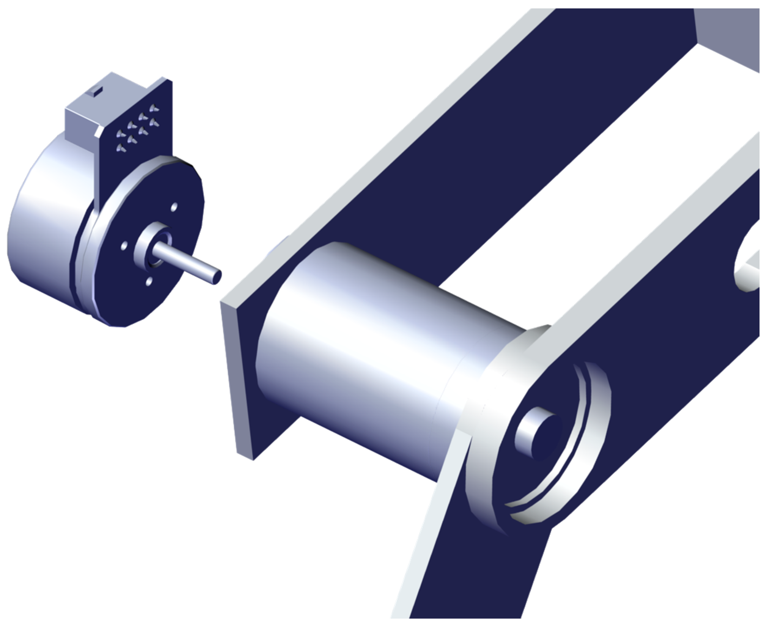
Figure 26.
Motor coupled to joint 2 (Ankle).


Table 1.
Generalized Hanavan model of the human leg.
| Limb Section | Parameters |
|---|---|
| Thigh | |
| Leg | |
| Foot |
where are the corresponding lower radii, are the higher radii, is the limb length, and is the height of the person (all in meters); is the density of the body in , is the segment mass, and is the person mass in [Kg].
© 2017 by the authors. Licensee MDPI, Basel, Switzerland. This article is an open access article distributed under the terms and conditions of the Creative Commons Attribution (CC BY) license (http://creativecommons.org/licenses/by/4.0/).
Share and Cite
MDPI and ACS Style
Velandia, C.C.; Tibaduiza, D.A.; Vejar, M.A. Proposal of Novel Model for a 2 DOF Exoskeleton for Lower-Limb Rehabilitation. Robotics 2017, 6, 20. https://doi.org/10.3390/robotics6030020
AMA Style
Velandia CC, Tibaduiza DA, Vejar MA. Proposal of Novel Model for a 2 DOF Exoskeleton for Lower-Limb Rehabilitation. Robotics. 2017; 6(3):20. https://doi.org/10.3390/robotics6030020
Chicago/Turabian StyleVelandia, Cristian C., Diego A. Tibaduiza, and Maribel Anaya Vejar. 2017. "Proposal of Novel Model for a 2 DOF Exoskeleton for Lower-Limb Rehabilitation" Robotics 6, no. 3: 20. https://doi.org/10.3390/robotics6030020
Note that from the first issue of 2016, this journal uses article numbers instead of page numbers. See further details here.