Design of a Mobile Robot for Air Ducts Exploration


Department of Electrical, Computer and Biomedical Engineering, University of Pavia, via Ferrata, 5-27100 Pavia, Italy
*
Author to whom correspondence should be addressed.
Robotics 2017, 6(4), 26; https://doi.org/10.3390/robotics6040026
Submission received: 3 July 2017
/
Revised: 25 September 2017
/
Accepted: 9 October 2017
/
Published: 11 October 2017
Abstract
:This work presents the solutions adopted for the design and the implementation of an autonomous wheeled robot developed for the exploration and mapping of air ventilation ducts. The hardware is based on commercial off-the-shelf devices, including sensors, motors, processing devices and interfaces. The mechanical chassis was designed from scratch to meet a trade-off between small size and available volume to host the components. The software stack is based on the Robot Operating System (ROS). Special attention was dedicated to the design of the mobility strategy, which must take into account some constraints and issues that are specific to the considered application, such as the relatively small size of ducts, the need to detect and avoid possible holes on the floor of the duct and other unusual obstacles and the unavailability of external reference frameworks for localization. The main contribution of this paper lies in the design, implementation and experimentation of the overall system.
1. Introduction
The use of autonomous mobile robots is spreading in many application domains due to their flexibility, mature off-the-shelf hardware and reusable software components and the general dropping of costs. Exploration of unknown, dangerous or inaccessible environments is among the most investigated and appealing application for autonomous robots. While mobile robots can adopt different approaches, technologies and techniques (see [1] for indications regarding a formal ontology to classify mobile robots), in particular to move on different terrains and surfaces, wheeled robots are among the most popular.
The application discussed in this paper refers to the exploration and mapping of air ventilation ducts by means of an autonomous wheeled mobile robot. The goal is to let the robot move autonomously through the ducts to collect information useful to realize a map of the duct, since rather often, such a map is not available or does not reflect the actual organization of the duct. The construction of the map is outsourced to the ROS navigation stack and is done in real time as the robot traverses the duct environment. A major application goal is to acquire video footage of the environment during the motion, which can be examined offline to detect obstructions and pollution, allowing the optimal planning of maintenance and cleaning operations. It is worth noting that the video is currently used for offline inspection after the robot completes the exploration task. On the other hand, the inclusion of a camera opens the door to the correction of errors in localization and mapping due to drifts in the robot wheels and subsequent errors in the encoder measurements with photogrammetric techniques [2].
This paper presents the design and implementation of a novel robot, discussing how the ROS navigation stack is leveraged to perform the exploration of the environment. The implemented motion strategy is based on discrete local steps (in the form of iterations) to incrementally explore the global space. The path planning is done by setting intermediate goal points using a method based on the centroid of free points in the operation space. This allows one to leverage the legacy navigation stack provided by ROS to move from one goal point to the next one. The exhaustive exploration of ducts is achieved by explicitly managing possible multiple branches in the tunnels. The exploration task is made challenging by the harsh duct environment, which is populated by several types of peculiar obstacles such as traps on the floor and thin suspended horizontal bars, as well as the lack of a global reference frame.
Since openings are often present in the floor of ducts where the robot is moving, trapdoor detection has a key role for the robot’s safety. The devised trapdoor detection approach is presented.
The proposed design and implementation have been evaluated by both simulations and experimental measurements. The effectiveness of the navigation method is shown by means of simulations on a realistic environment, while an evaluation of the overall processing capability requirements has been assessed on the implementation of the software stack on the adopted computational devices.
Article Organization
Relevant related works are reported in Section 2. The presentation of the project addresses the hardware platform and the software stack, presented in Section 4 and Section 5, respectively. Section 6 discusses the overall trajectory planning and navigation approach, while Section 7 focuses on the algorithm developed specifically for this use case. Experimental results and evaluations are reported in Section 8, and concluding remarks are stated in Section 9.
2. Related Work
Autonomous robot navigation has been an important area of research in the past few decades [3,4], and mobile robots play a significant role in today’s world, ranging from military to consumer applications. The research on autonomous mobile robots developed to navigate in special indoor environments spans from general exploration tasks [5] to special applications such as fire fighting in tunnels [6] or archaeological exploration [7].
In [8], the authors describe an autonomous robotics platform for the exploration of caves and mines. While some localization challenges are common to our addressed scenario, several aspects are peculiar to their specific application environment. The research in [9] presents the construction aspects of an autonomous caterpillar vehicle developed for exploring tunnels in dangerous conditions, i.e., where poisonous gases or other threats are present.
In [10], there is an analysis of the challenges related to robot operations in subterranean and harsh scenarios. The identified challenges include autonomous navigation, localization, mapping and communication. Sensors and mapping techniques play a key role in the development of an efficient robotic exploration application in constrained environment. The case for this work requires a robot to autonomously navigate within ventilation ducts without the use of a Global Positioning System (GPS) as a global reference frame since GPS signals are inaccessible. While [11] analyzes recent advances in both domains, [12] presents a localization approach based on a strap-down Inertial Measurement Unit (IMU). In terms of navigation challenges, [13] provides a method to detect the walls in a corridor to enable an efficient navigation of a mobile robot, and [14] focuses on the mapping of large-scale underground environments. The present work focuses instead on ventilation ducts, which typically have a relatively small scale.
Autonomous navigation of robots in GPS-denied environments with ventilation ducts is a currently explored area of research. In the recent past, mobile robots have been controlled using cables as with Remotely Operated Vehicles (ROV), using umbilical cords [15]. These cables supply power and serve as channels for telemetry. The main bottleneck with tethered robots is that the cable length limits the operational range of the robot. The advantages of tethering sometimes outweigh the inherent limitation of bounded coverage, as seen in [16]. Similar approaches use line following algorithms where the robot is equipped with an array of infrared sensors that center the robot’s motion with respect to a line drawn on the floor of the environment [17]. This method requires an existing line to be drawn across the entire exploration space, limiting the flexibility of the approach.
3. Robot Model
The 3D rendering of the robot is shown in Figure 1a,b. Some considerations about the solutions adopted for the mechanical frame, with special attention to obstacle detection and robot safety issues, are reported. However, the core of this work is dedicated to the selection and integration of electronic hardware components and to the development of the onboard software stack, which is based on the Robot Operating System (ROS) [18].
The main project goal is the small size (the prototype is cm), since the robot must be able to move in relatively small ducts. The battery life is not critical; a target value is around one hour, which can be achieved with standard batteries without major issues on power-awareness in the robot’s electronics or mobility strategy. Traveling speed is also non-critical. The robot peak velocity can be as low as 5–10 cm/s. As a target design goal, the length of the path to explore ranges between 20–30 and 250–300 m.
The robot is equipped with different sensors that allow it to interact properly with the unknown ventilation ducts and achieve the overall exploration goal. The hardware setup includes a laser scanner, two infrared sensors for specific obstacle detection, a strap-down Inertial Measurement Unit (IMU) and two wheel encoders.
The entire logic related to the movement of the robot has been outsourced to the ROS navigation stack, which is described later in Section 6. The robot is a differential drive robot, where each wheel is powered by an independent DC motor, while quadrature encoders provide angular displacement measurements (more details in Section 4). The robot is able to maneuver in response to commands provided by the navigation stack. In particular, the robot can easily rotate over its center of mass to make a u-turn, while it can move backward provided the right set of commands is given to the wheel motors by the navigation stack.
Robot Communication
The robot is intended to explore the duct environment autonomously. It is thus not tethered. It was initially supposed to maintain a wireless communication between the robot and a base station, so that the robot could transmit information via ROS’ networking framework and robot joint position and mapping progress could be visualized on the control station using rviz, an ROS package that provides robot visualization capabilities. However, upon the discovery that wireless signals perform poorly in the ducts, which are typically made of metallic materials, this requirement was suppressed. To ensure that the robot can be easily recovered in case of errors or system exceptions that would bring the robot to a halt, the robot is fitted with buzzers that sound periodically. The robot can then be easily recovered by a human following the sound of the buzzers or the light from the LEDs to locate the robot in the duct in case of emergency. We here note that a preliminary recovery is attempted by the robot (described in Section 6.1.5), whose failure leads to the need for a manual recovery.
4. Hardware Setup
The hardware setup is composed by several devices, sensors and actuators, controlled by a Single Board Computer (SBC). The SBC used in the actual implementation is a Raspberry Pi 2. Figure 2 shows a scheme of the devices connected to the SBC and the communication interfaces supporting each connection.
The main components are the following:
- A Hokuyo laser scanner (Hokuyo urg-04lx-ug01): It is connected via a Y-cable Universal Serial Bus (USB) connector to the Single Board Computer (SBC).
- A quadrature encoder board: The board uses dedicated hardware to read the signals from the encoders installed on one left and right wheel; the communication with the quadrature encoder is via the Serial Peripheral Interface (SPI) bus.
- Two incremental encoders connected to the quadrature encoder.
- Two micro-switches are mounted on the front sweeping arm. Connected to the SBC through General Purpose Input/Output pins (GPIO), they are sampled to detect a possible front collision of the vehicle. The two switches act as a logical OR, such that at least one of them needs to be pressed to detect a collision.
- An Inertial Measurement Unit (IMU), which communicates with the SBC via the I2C bus.
- A hole detector sensor: It is an Infrared proximity sensor (IR) mounted beneath the front edge of the sweeping branch. It is sampled to detect the presence of holes placed under the sensor. It is connected to the SBC via I2C.
- A PiCamera is used for video capture. It communicates with the dedicated Camera Serial Interface (CSI) available on the Raspberry Pi board.
- A custom Light-Emitting Diode (LED) control Printed Circuit Board (PCB) is connected via a General-Purpose Input/Output (GPIO) pin that generates a software PWM (created with a driver called pigpio).
- A motor control PCB: Connected via two GPIOs, it produces two independent Pulse-Width Modulation (PWM) signals, independent of the SBC processing. This dedicated hardware uses much less computing power with respect to to the PWM implemented via the software driver, which has a processor utilization of around .
- A USB memory drive to save the camera footage and make it easily copyable to a computer.
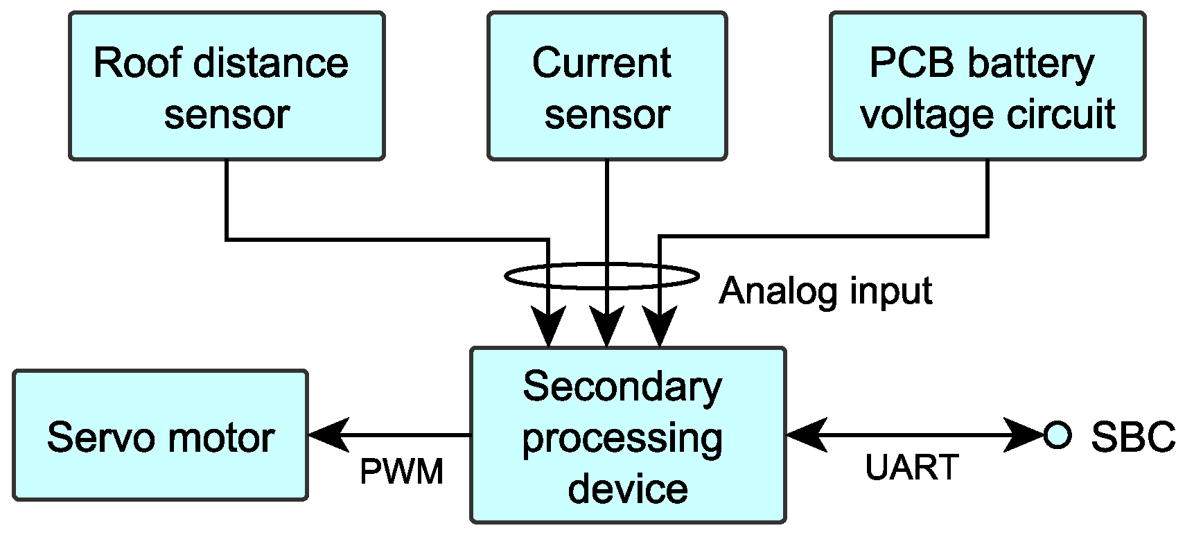
Since the adopted SBC (i.e., Raspberry Pi) lacks analog interfaces, there is a micro-controller-based board (Arduino Trinket Pro) that controls the servo motor connected to the robot’s sweeping arm by means of a PWM signal and that reads the signals of the analog sensors. Figure 3 shows a block schema describing how the Trinket Pro (indicated as the secondary processing device) is connected to the SBC and other analog interfaces.
Obstacle Detection
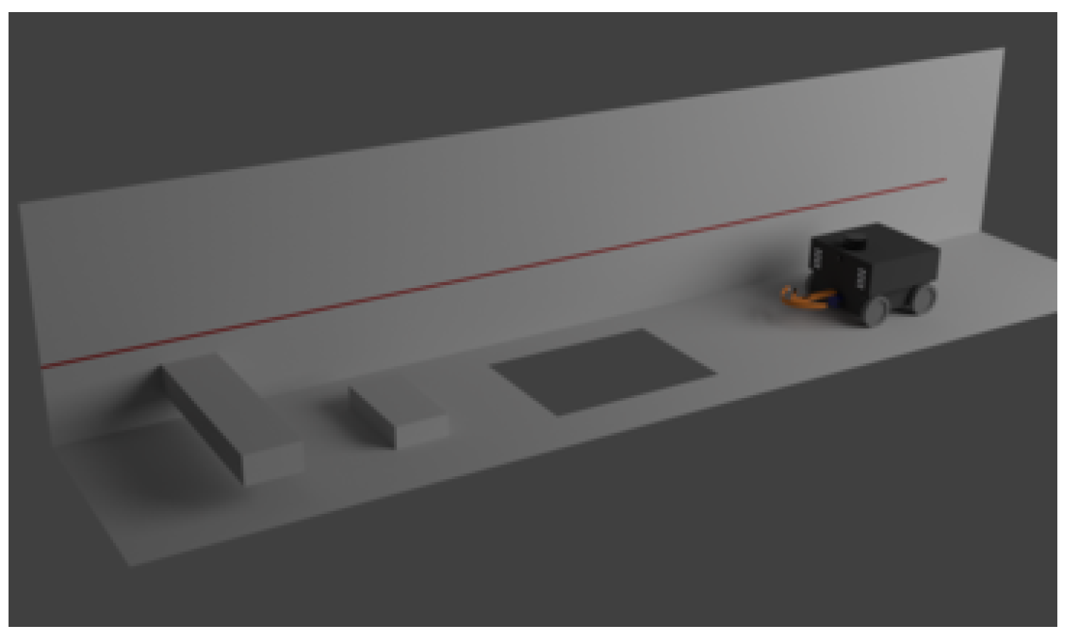
While the laser sensor offers a great source of data for localization, Figure 4 shows how the environment where the robot moves can make it face obstacles that the laser sensor cannot detect. Indeed, if the obstacle does not lay in the sensing plane of the laser scanner, it will not be detected.
In addition to the walls that are detected by the laser sensor itself, the obstacles the robot can face are trapdoors or, in general, holes in the floor, bumps, short obstacles and horizontally-suspended ones. Figure 4 shows an example of these possibilities.
A possible solution could be to employ a rotating laser scanner with the sensing plane not parallel to the floor plane, or to use more than one scanner. Although these solutions are widely considered for similar situations, the simple nature of the environment and the finite number of obstacle types the robot can face led to the use of simpler and much less expensive sensors.
The trapdoor sensor, the micro-switches and the roof distance sensor are used to detect holes, bumps and suspended obstacles, respectively. These sensors are mounted on an arm connected to the main body by a servo motor. The arm is able to sweep over the whole width in front of the vehicle. This approach allows one to detect obstacles before they collide with the front side of the robot; trapdoors are detected before the front wheels fall into them. Since during its sweeping, the arm may collide with an obstacle, the contact sensor located on the front edge of the arm, and implemented using the micro-switch, allows detecting possible collisions of the edge. The adopted solutions allow a complete detection of possible obstacles and holes that may appear in front of the robot during its motion. The early detection of an impeding object allows the robot to promptly stop its motion.
Once an obstacle or trapdoor is detected and the robot is stopped, the sweeping arm could also be used to map the impeding object, so that the robot can eventually determine its size and shape and figure out whether the robot can navigate around it.
5. Software Stack
The software stack is built on top of the Robot Operating System (ROS). An ROS application is made of different processes, called nodes, which communicate by exchanging messages (topics). In the implemented application, the values obtained from sensor sampling are translated into ROS topics to simplify the access from nodes implementing the robot behavior. Similarly, control signals are first sent as ROS topics and then translated in hardware signals by specific nodes. This section explains and analyzes the most interesting processes, which are grouped according to the corresponding specific task.
5.1. Hardware Interfaces
There are several different interfaces between the SBC and the actual hardware. The data provided by the laser scanner are read by the hokuyo_node and passed via the /map topic to the slam_gmapping node, which in turn localizes the robot using SLAM with respect to a global reference frame.
Acceleration and angular velocity are read by imu_reader and transferred to the SBC via I2C. The data are filtered by imu_filter, before being published on the /imu topic. Data from the encoders are received by the robot_odom node from the quadrature_encoder node, which in turn exploits the spi_driver to communicate with the quadrature encoder hardware device.
The robot_bumper node, using the gpio_driver, monitors the status of the switch and publishes on topic /collision in case a collision is detected; this information is used to stop the robot. In the same way, the ir_short node uses I2C_driver for reading the trapdoor IR sensor. A topic is published to stop the robot when a trapdoor is sensed. ir_long is the node that receives the raw data of the ceiling distance sensor. It then publishes the actual distance from the ceiling through the linearization node.
led_controller allows turning the LEDs on and off. It operates on the LED status by means of a PWM signal created using the pwm_driver_rasp library. The motors_controller node receives linear and angular velocities from the navigation stack and translates them into PWM signals that are sent to the motor controller bridge. The servo_motor node calculates the servo motor angle and publishes it in order for the Trinket Pro to actually control the servo motor by means of a PWM signal. While the PWM signal is carried by the Trinket Pro in order to lower the amount of load on the Raspberry, the latter calculates the servo position. The position is needed by the system in order to know the position of the sweep branch relatively to the robot body frame.
The current_sensor nodes is responsible for publishing the battery voltage topic, the amount of consumed current and battery power information. The calculations for these data are done by the secondary processing device. This node takes the data via ros_serial from it and publishes them on the system topics.
Interfacing New Hardware
The current robot setup can be extended by adding new hardware in order to fit the robot with more capabilities. In terms of hardware/software setup, to allow communication between the new hardware and the existing robot setup, it is sufficient to write an ROS node that communicates with the driver of the new hardware. The new node will be a subscriber that reads data from existing topics and takes action accordingly (e.g., for new hardware that is an actuator), or a publisher that publishes data supplied by the new hardware, in the case of new hardware that is a sensor, which can then be consumed by parts of the setup that need these data. From the mechanical viewpoint, however, new hardware can only be added if it fits into a chassis that is already optimized to contain the necessary components and properly dimensioned to allow the robot to enter relatively small ducts.
5.2. Localization and Mapping
The localization and mapping parts of the setup are essential to the completion of the exploration and mapping objective of the robot. The logic for the localization of the robot has been outsourced to ROS’s robot_localization node, which provides nonlinear state estimation through sensor fusion of the available sensors. It uses an extended Kalman filter as described in [19], in our case combining IMU samples, laser scans and odometry information. The odometry due to the non-uniform friction in the ventilation ducts suffers from slippage propagated from the encoder measurements; the IMU suffers from noise and drift; while the laser scanner strives to make accurate ranging measurements when the robot is traveling along a lengthy stretch of tube. Fusing all the sensor information together with the Extended Kalman Filter (EKF), the error from one source is compensated by integrating from the others. Using the static transformations published by robot_tf, the robot_localization node maintains a coherent geometry, e.g., the position of the laser scanner with respect to the robot body frame.
Once these data are combined, the robot_localization node publishes the position of the robot with respect to a global /odom reference frame. Using SLAM, the tf transformation that renders the two global reference frames—/odom and /map—coherent can also be published. This allows letting the robot move using one reference frame, while maintaining coherent knowledge of the space around the robot with respect to the two frames. Figure 5 shows the setup of the localization stack for the robot. Drivers and hardware devices are depicted with rectangles in dashed-lines, ROS nodes with rectangles in continuous lines and ROS messages with ellipses.
The SLAM operation is performed by the slam_gmapping node, which is fed by ranging information from the Hokuyo laser scanner and odometry information from the sensors data that robot_localization combines. As the robot moves in the duct environment, a 2D occupancy grid map is generated by slam_gmapping, which can later be exported in a suitable image format after the exploration is complete. Since the map creation and storage are handled by ROS, partial maps of the already performed exploration are available in case of emergencies where the robot stops or shuts down arbitrarily. To read raw laser scans, the hokuyo node performs periodic reads from the Hokuyo laser scanner and publishes ranging information to the hokuyo topic, which is consumed by slam_gmapping. The latter in turn generates the map and publishes the /map topic. Figure 6 shows the components of the mapping framework and how they are connected. The odometry topic depicted in Figure 5 is also fed into the slam_gmapping node to be integrated with other sensory information.
6. Trajectory Planning and Navigation
The global exploration task is formulated as a sequence of successive local problems. The robot is required to move in small steps.
ROS uses information from costmaps to provide the localization data required by its trajectory planners. A costmap is an occupancy grid corresponding to a physical area in the environment. The grid consists of cells that have costs indicating the status of a sub-area in the environment, which can either be occupied, free or unknown. Cells are marked as occupied or cleared as free using information from the robot’s sensors. Sensors are seen as topic publishers providing the relevant data to the navigation stack. In each local step, the following actions occur (in the given order):
- goal pose is computed;
- the computed pose is sent to the ROS navigation stack;
- the ROS base_local_planner (a node in the navigation stack) computes a path to reach the goal;
- ROS move_base (another node in the navigation stack) sends the motion control sequence for following the path and responds with success (or failure) at the end;
- if the path following operation succeeds, the robot computes the next goal pose;
- this process is repeated until the duct space has been completely explored or some higher priority condition is triggered, such as the low battery indication.
Our setup uses three costmaps: a local and a global costmap for local and global trajectory planning and a custom costmap for the goal pose estimation. The robot’s global movement is discretized into steps whose intervals are bounded by the maximum displacement of a goal from the current location of the robot within an instance of the custom costmap.
6.1. High Level Robot’s Behavior
Ventilation ducts include different topological features, namely: freeway, branch/crossroad, hole/trapdoor and dead-end, as depicted in Figure 7.
The robot behavior is dictated by a Finite State Machine (FSM) that captures all known possible scenarios within a ventilation duct. Figure 8 shows the organization of the FSM. The set of states composing the FSM, their meaning and their relationships are explained in the following.
6.1.1. State : Snooze
The Snooze state is an abstraction that models the intermittent stops between two consecutive instances of the Navigate state. The time spent in an instance of this state is equivalent to the time taken by the duct navigation node to refresh the custom costmap and compute a new goal pose for the ROS navigation stack.
6.1.2. State : Navigate
The Navigate state is the most crucial state in the FSM. It defines the interaction between the navigation algorithms described in Section 7 and the ROS navigation stack. Empirically, the robot spends about 90% of its exploration time in this state, switching back and forth between Navigate and Snooze states. In this state, the robot attempts to reach the target goal computed by the navigation algorithm using the custom costmap. In the execution of this state, a few exceptions could be encountered as indicated in Figure 8:
- The robot is stuck since the base_local_planner drove the robot too close to an adjacent wall while approaching a bend; the robot is unable to move further given the constraints of its inflation radius or when the robot has reached a dead-end. The actions taken to face this condition are described in Recovery.
- The robot detects a trapdoor opening/hole in which case the state changes to Hole Area.
When the exploration is deemed complete according to a set criteria described in Section 7, the state changes to Return. Thanks to the inflation radius set around the robot footprint by the navigation stack in the costmap, the robot does not proceed into spaces narrower than its width. In fact, when the inflation radius intersects with a wall of such spaces on entry, the wall is deemed an obstacle.
6.1.3. State : Hole Area
On reaching this state, the robot runs a procedure that marks as dangerous the cells in the local and global costmaps corresponding to portions of the hole that are reachable by the sweeping arm. Although it is desirable to devise a procedure that would allow the robot to evade the hole (i.e., circumnavigating it) and continue the exploration, this requirement was suppressed upon the knowledge that most holes in a ventilation duct network span the entire width of the duct itself, making it impossible for the robot to circumnavigate it. Hence, the robot only maps the hole area (seen by the IR sensor on the robot’s sweeping arm) as occupied/dangerous, considers the associated duct section as a dead-end and turns around to continue to the next goal in the exploration stack (see Section 7). Alternatively, it switches to the Return state if the exploration stack is empty.
6.1.4. State : Return
In this state, the robot returns to the its global start position at the end of the exploration task. This is an oversimplification of the Navigate state, as no goal is computed, and the navigation algorithm simply gives base_local_planner a goal equivalent to the starting pose. The successful execution and transition of this state into the final Snooze state depends greatly on the accuracy of our localization. If the drift in odometry readings for example is too large, the robot might end up in a position that is several tens of centimeters away from the original starting position. In such cases, as stated in Section 3, the robot can be located in the duct using the sound from the buzzer and/or the light from the LEDs and recovered manually. On the other hand, when the return-home task begins, the robot exploration is already deemed complete. Therefore, it would not be required to have an accurate map or to perform any mapping at all during the robot’s return to home.
6.1.5. State : Recovery
As discussed regarding the Navigation state, the Recovery state handles both cases where the robot is stuck or a dead-end has been reached.
When the robot is stuck, rotate_recovery, a ROS package that provides a simple recovery behavior that rotates the robot (if local obstacles permit) in an attempt to clear and free neighboring cells in the navigation stack’s costmaps, is invoked by the Navigation stack.
The recovery action for a dead-end is to backtrack the robot by a few centimeters, perform an in place rotation of , after which the robot proceeds to the next goal position in the exploration stack (discussed in Section 7). Before the robot is backtracked, the sweeping arm is retracted close to the robot to create more allowance for the rotation and clear the sweeping arm and chassis from any collisions while rotating. A dead-end is flagged either by a collision on any of the micro-switches or most often after computing the relative displacement between successive goal positions in the custom costmap; once the displacements are seen to converge towards zero, it implies that the custom costmap is not being updated with new free cells while the old ones are being depleted as the robot moves further away from them. The Recovery state is reachable from the Navigate and Return states.
7. Navigation Algorithm
The approach developed for the autonomous navigation of the mobile robot in the ventilation ducts is called Map Edge.
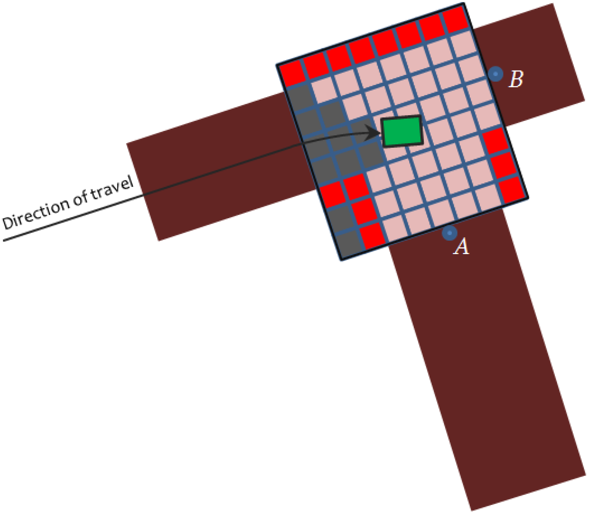
The Map Edge approach initializes the custom costmap, scans the entire perimeter of the map moving anticlockwise from the origin: up, left, down, and right, in this order. The points marked as free on this perimeter are collected. These points are clustered by checking for point-wise discontinuities along the x and y coordinates of the cells; each discontinuity marks the boundaries of a potential branch. The coordinates of the cells in each cluster are averaged, to select a goal point for each branch. In the event more than one branch is detected after clustering (implying the robot is at a crossroad), the algorithm needs to memorize the branching points that have yet to be visited by the robot. From Figure 9, if the robot takes branch A first, it has to memorize branch B, and in the case where more branches are detected while a branch is currently being explored, all unvisited branches are altogether cached in the exploration stack. When branches are detected/scanned at a crossroad, the edges of the immediate costmap are scanned in an anticlockwise fashion (see Algorithm 1). Openings in the edge (i.e., detected branches) are added to the exploration stack in the order in which they are detected. The branch that is first visited after the detection task is complete is the one at the top of the stack (i.e., the branch that was lastly added), which is usually the leftmost branch at the crossroad with respect to the robot; scanning was done in an anti-clockwise fashion.
The depth first algorithm is used for revisiting nested branches. Algorithm 1 provides the mathematical details of the algorithm.
| Algorithm 1 Map Edge navigation algorithm. | |
| Input: costmap-boundary, global-stack | |
| Output: | |
| 1. | |
| 2. | |
| 3. for all do | ▹ scan/iterate in anticlockwise |
| 4. if free space then | |
| 5. | |
| 6. end if | |
| 7. end for | |
| 8. if then | |
| 9. for all do | |
| 10. | |
| 11. while and are neighbors do | |
| 12. | |
| 13. end while | |
| 14. | |
| 15. | |
| 16. end for | |
| 17. | |
| 18. | |
| 19. else | ▹ Dead end reached |
| 20. if then | |
| 21. | |
| 22. else | |
| 23. | ▹ Exploration complete |
| 24. end if | |
| 25. end if | |
| 26. return goal | |
From Algorithm 1, it can be observed that two stacks are managed:
- Branches detected from any iteration of the algorithm are pushed into the local stack. This is not emptied until the start of the next iteration before which the costmap is reset.
- Updates from the local stack are appended to the global stack. Hence, the global stack caches all the branching points, which are yet to be explored. As soon as a branch has been completely explored, its corresponding branching point is popped off, and the next branching point in the stack becomes the new goal pose.
When not at a crossroad, every new iteration assumes that the robot is traveling through the same branch. For this reason, no caching is performed. The area of the costmap is set to fall within the range of the laser scan while the width is set to be larger than the maximum width of the duct at any point (see Figure 9). This is to ensure that crossroads in the duct environment have all their branches detected so as to be included in the exploration stack maintained by the algorithm. If the custom costmap area is too small, the robot will have a blind-spot for branching points. The only constraint to this could be the range of the laser scanner, which is however usually sufficiently large. Figure 9 shows the robot marking the centroids of two branches as the next potential goal positions.
8. Experimental Evaluation
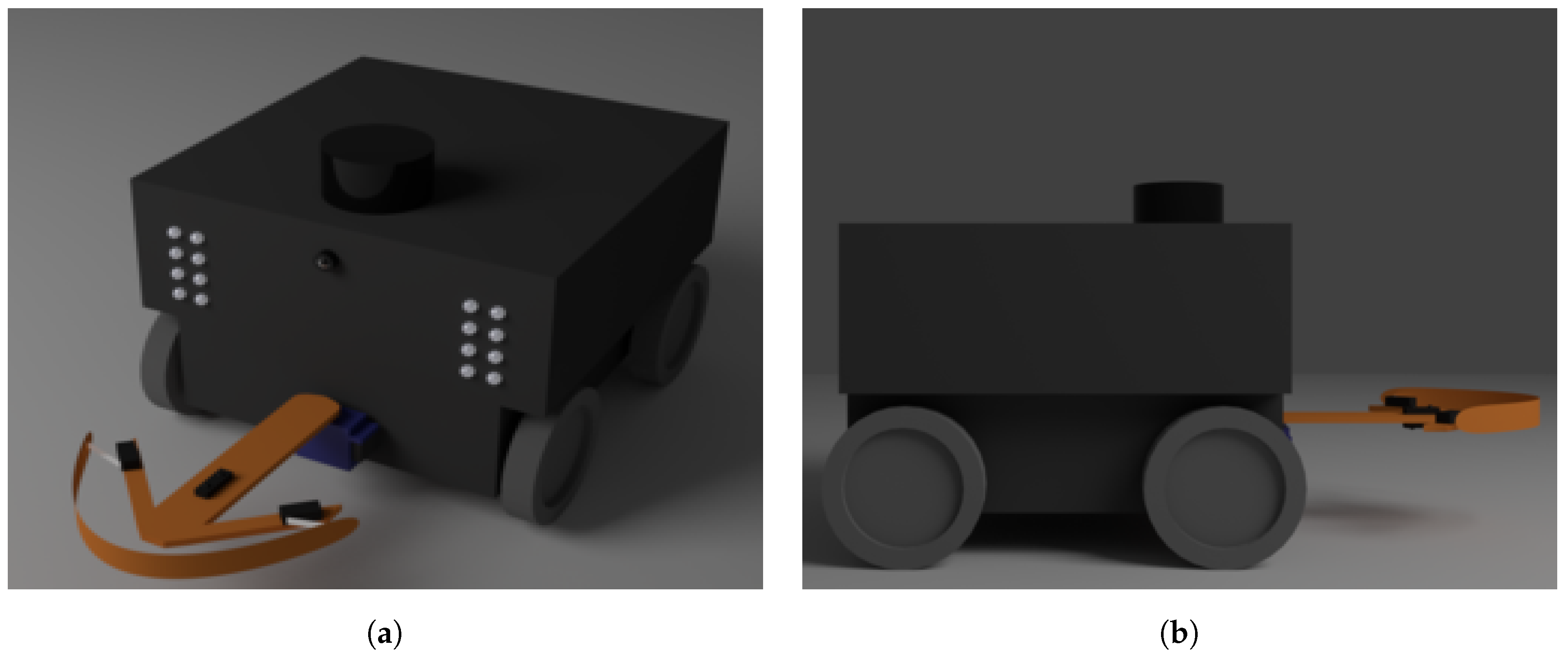
This section reports some experimental assessments made on the developed platform. An image of the physical robot is shown in Figure 10.
One main concern in this application is the complexity of the software application, which is evident from the number of ROS nodes and functionalities that have been implemented. For this reason, special attention was paid to profiling the computational load due to these nodes on the actual SBC. The problem is related to the tradeoff between a low power-consuming SBC and its relatively limited processing capability. Table 1 shows the list of nodes running on the SBC and their processor usage. ros_launch and ros_master, which are not considered as ROS nodes, are added to the table to help better understand how the processor allocates resources for default ROS processes alongside other nodes in a typical setup.
As can be noticed, most of the computation refers to the sensor fusion, while another heavy process is due to the IMU data reading and filtering. Almost all the other activities have a negligible impact on the processor utilization.
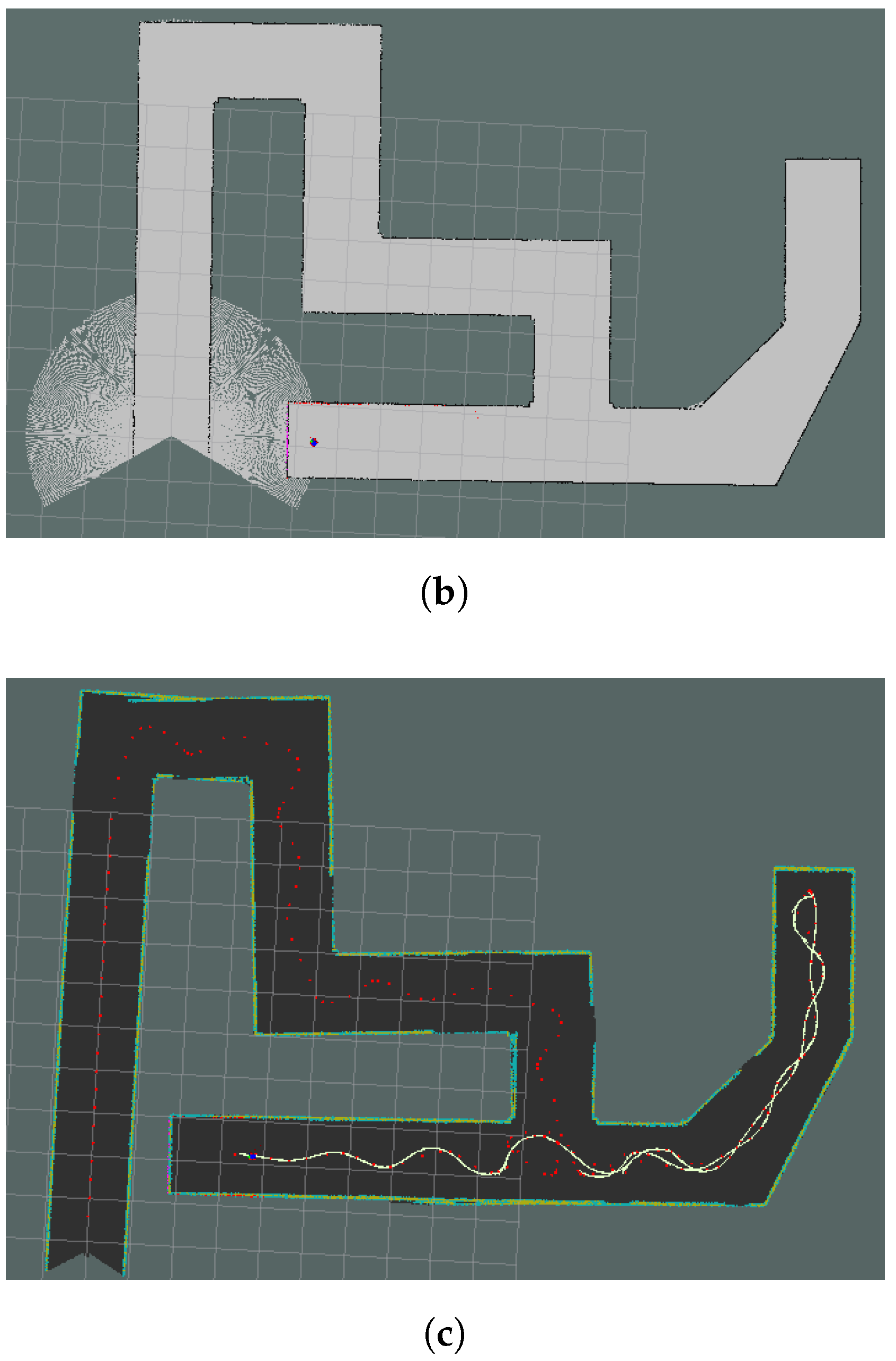
Several tests were also carried out on the suitability and the effectiveness of the navigation algorithm. Two examples of the execution of the exploration task are reported. Figure 11 shows the behavior in a relatively simple environment, without obstacles and branches. Afterwards, a more advanced duct environment is considered, having typical features of a real ventilation duct such as the crossroad and dead-end shown in Figure 12a. The simulation environments were created in the Gazebo simulator, while the maps were taken from the ROS RVIZ (Robot Visualization tool). Holes were not included in the environment since the default action after detecting a hole is to terminate the pursuit of the current goal point, push the goal point off the stack and then pursue the topmost (or next) available goal position in the stack. Mapping results for two duct environments are shown in Figure 11 and Figure 12. The red markers are goal points selected by the navigation algorithm in use. The lines trailing the robot were traced from these markers, and they indicate the robot path. In both cases, the robot succeeds in fully exploring the environment, building a reliable map of the unknown area.
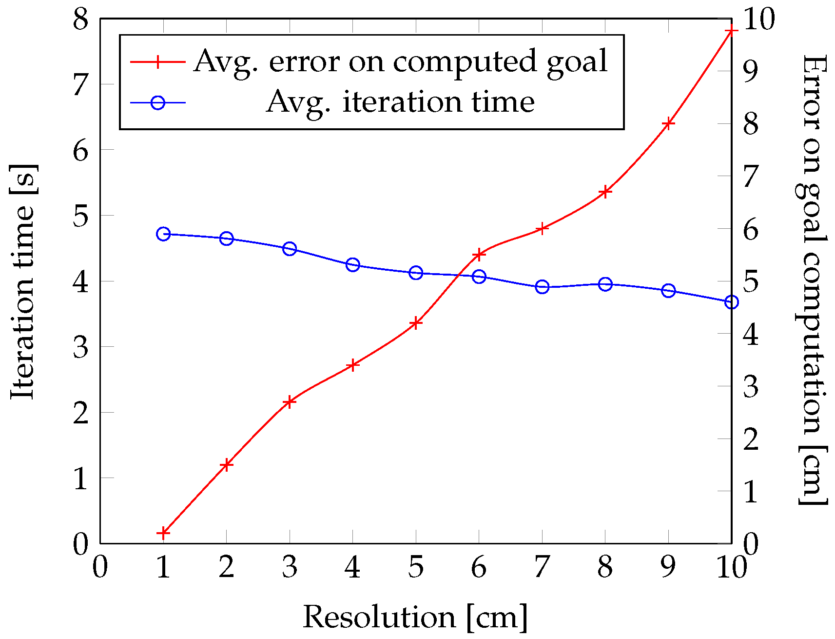
Since the value of the costmap resolution is not fixed and should be selected by the user, to ease the selection of a suitable costmap resolution, more experimental results are provided in Figure 13 showing two graphs. The first graph in blue shows the average iteration/exploration time (i.e., time for goal computation plus robot transit time to reach the goal) against costmap resolution. The second graph in red shows the average error on reaching the computed goal against costmap resolution.
The graphs were plotted by averaging 20 runs of the robot exploration in the environment in Figure 11c, increasing the resolution from 10 cm to 1 cm in steps of one. From the graphs, the increase in error as the resolution of the costmap reduces is noticeable, while the slightly increased average exploration time for higher resolutions is also noticeable. Therefore, a good compromise between average time to complete an exploration and the accuracy of the robot movement/transitions will mean selecting a costmap resolution of about 5 cm.
9. Conclusions
This paper presented the design and the implementation of an autonomous wheeled robot meant for the exploration of air ventilation ducts. The presentation included the hardware and the software stack, with discussions on the adopted methods. Part of the focus was on the navigation, obstacle detection and avoidance approaches, which have some peculiarities related to the specific working environment. The adopted navigation approach, hardware or software architectures can be extended for more complicated environments or, alternatively, simplified for environments that are relatively less complicated. The setup emphasizes the use of off-the-shelf devices to ease the replicability of the entire setup. The modeling of the robot, the environment and the navigation algorithm were equally done with free and open source software, consistent with the aforementioned objective of replicability. The implemented solutions were validated both by simulation and with processor load measurements on the developed robot.
A drawback of this work is the unavailability of a global localization reference, as such errors in localization keep increasing. Approaches to reduce the growth rate of the error can be considered as the integration of the video capture into the localization system. Another drawback is that the accuracy of the system as reported in this work does not include practical experiments. On the other hand, despite these limitations, this work proposes a relatively inexpensive and easy to deploy solution for autonomous robot exploration of ventilation ducts and similar spaces. The simulations also provides a setup for rapidly prototyping our solution in other similar environments.
Acknowledgments
This work was partly funded by Alisea s.r.l.
Author Contributions
Moses A. Koledoye conceived of the navigation algorithm. Massimo Carvani designed the hardware and software architectures. Daniele De Martini designed the robot model. Moses A. Koledoye and Massimo Carvani performed the experiments. All authors contributed to the paper.
Conflicts of Interest
The authors declare no conflict of interest.
Abbreviations
The following abbreviations are used in this manuscript:
| CSI | Camera Serial Interface |
| FSM | Finite State Machine |
| GPIO | General Purpose Input/Output |
| GPS | Global Positioning System |
| I2C | Inter-Integrated Circuit |
| IMU | Inertial Measurement Unit |
| IR | Infrared |
| PCB | Printed Circuit Board |
| PWM | Pulse Width Modulation |
| ROS | Robot Operating System |
| ROV | Remotely-Operated Vehicle |
| SBC | Single Board Computer |
| SLAM | Simultaneous Localization And Mapping |
| UART | Universal Asynchronous Receiver/Transmitter |
References
- Bayat, B.; Bermejo-Alonso, J.; Carbonera, J.; Facchinetti, T.; Fiorini, S.; Goncalves, P.; Jorge, V.A.; Habib, M.; Khamis, A.; Melo, K.; et al. Requirements for building an ontology for autonomous robots. Ind. Robot Int. J. 2016, 43, 469–480. [Google Scholar] [CrossRef]
- Pierce, S.; Dobie, G.; MacLeod, C.N.; Summan, R.; Baumanis, K.; Macdonald, M.; Punzo, G. Visual asset inspection using precision UAV techniques. In Proceedings of the 11th European Conference on Non-Destructive Testing, Prague, Czech, 6–10 October 2014. [Google Scholar]
- Bourbakis, N. Design of an autonomous navigation system. IEEE Control Syst. Mag. 1988, 8, 25–28. [Google Scholar] [CrossRef]
- Wallgrün, J.O.; Oliver, J. Hierarchical Voronoi Graphs: Spatial Representation and Reasoning for Mobile Robots; Springer: Berlin, Germany, 2010; pp. 14–15. [Google Scholar]
- Loupos, K.; Amditis, A.; Stentoumis, C.; Chrobocinski, P.; Victores, J.; Wietek, M.; Panetsos, P.; Roncaglia, A.; Camarinopoulos, S.; Kalidromitis, V.; et al. Robotic intelligent vision and control for tunnel inspection and evaluation—The ROBINSPECT EC project. In Proceedings of the IEEE International Symposium on Robotic and Sensors Environments (ROSE), Timisoara, Romania, 16–18 October 2014; pp. 72–77. [Google Scholar]
- Celentano, L.; Siciliano, B.; Villani, L. A robotic system for fire fighting in tunnels. In Proceedings of the IEEE International Safety, Security and Rescue Rototics, Workshop, Kobe, Japan, 6–9 June 2005; pp. 253–258. [Google Scholar]
- Wang, J.; Zhu, X.; Tie, F.; Zhao, T.; Xu, X. Design of a modular robotic system for archaeological exploration. In Proceedings of the IEEE International Conference on Robotics and Automation (ICRA’09), Kobc, Japan, 12–17 May 2009; pp. 1435–1440. [Google Scholar]
- Bakambu, J.N.; Polotski, V. Autonomous system for navigation and surveying in underground mines. J. Field Robot. 2007, 24, 829–847. [Google Scholar] [CrossRef]
- Zhuang, F.; Zupan, C.; Chao, Z.; Yanzheng, Z. A cable-tunnel inspecting robot for dangerous environment. Int. J. Adv. Robotic Syst. 2008, 5. [Google Scholar] [CrossRef]
- Murphy, R.R.; Kravitz, J.; Stover, S.L.; Shoureshi, R. Mobile robots in mine rescue and recovery. IEEE Robot. Autom. Mag. 2009, 16, 91–103. [Google Scholar] [CrossRef]
- Leingartner, M.; Maurer, J.; Ferrein, A.; Steinbauer, G. Evaluation of Sensors and Mapping Approaches for Disasters in Tunnels. J. Field Robot. 2016, 33, 1037–1057. [Google Scholar] [CrossRef]
- Xiong, C.; Han, D. An integrated localization system for robots in underground environments. Ind. Robot Int. J. 2009, 36, 221–229. [Google Scholar] [CrossRef]
- Larsson, J.; Broxvall, M.; Saffiotti, A. Laser-based corridor detection for reactive navigation. Ind. Robot Int. J. 2008, 35, 69–79. [Google Scholar] [CrossRef]
- Zlot, R.; Bosse, M. Efficient Large-scale Three-dimensional Mobile Mapping for Underground Mines. J. Field Robot. 2014, 31, 758–779. [Google Scholar] [CrossRef]
- Whitcomb, L. Underwater robotics: Out of the research laboratory and into the field. In Proceedings of the IEEE International Conference on Robotics and Automation (ICRA’00), San Francisco, CA, USA, 24–28 April 2000; Volume 1, pp. 709–716. [Google Scholar]
- Kim, S.; Bhattacharya, S.; Kumar, V. Path planning for a tethered mobile robot. In Proceedings of the IEEE International Conference on Robotics and Automation (ICRA’14), Hong Kong, China, 31 May–7 June 2014; pp. 1132–1139. [Google Scholar]
- Colak, I.; Yildirim, D. Evolving a Line Following Robot to use in shopping centers for entertainment. In Proceedings of the 35th Annual Conference of IEEE Industrial Electronics (IECON’09), Porto, Portugal, 3–5 November 2009; pp. 3803–3807. [Google Scholar]
- Quigley, M.; Conley, K.; Gerkey, B.P.; Faust, J.; Foote, T.; Leibs, J.; Wheeler, R.; Ng, A.Y. ROS: An open-source Robot Operating System. In Proceedings of the ICRA Workshop on Open Source Software, Kobe, Japan, 12–17 May 2009. [Google Scholar]
- Moore, T.; Stouch, D. A Generalized Extended Kalman Filter Implementation for the Robot Operating System. In Proceedings of the 13th International Conference on Intelligent Autonomous Systems (IAS’13), Padova, Italy, 15–18 July 2014. [Google Scholar]
Figure 1.
The 3D rendering of the robot.: (a) front view; (b) side view.

Figure 2.
Block diagram showing the hardware components of the robotics platform, including sensors, actuators and the adopted interfaces.
Figure 2.
Block diagram showing the hardware components of the robotics platform, including sensors, actuators and the adopted interfaces.
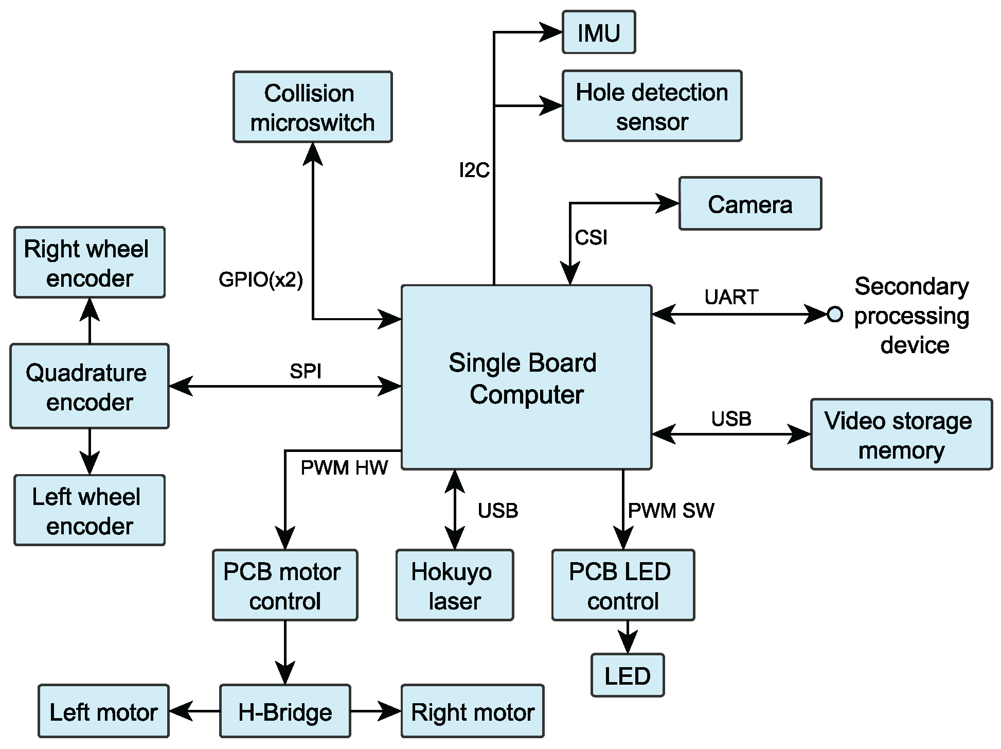
Figure 3.
Block diagram showing the components handled by means of an analog interface.

Figure 4.
Example of an environment with obstacles. From left to right: horizontally-suspended obstacle, short obstacle and a trapdoor.
Figure 4.
Example of an environment with obstacles. From left to right: horizontally-suspended obstacle, short obstacle and a trapdoor.

Figure 5.
Components of the robot localization stack.

Figure 6.
Components of the mapping stack.

Figure 7.
The layouts that can compose a typical air ventilation duct. The walls and roof of the duct are not shown.
Figure 7.
The layouts that can compose a typical air ventilation duct. The walls and roof of the duct are not shown.
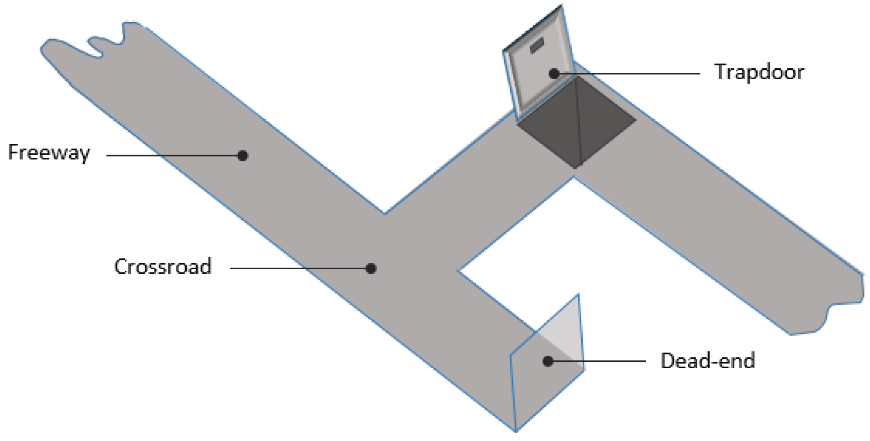
Figure 8.
Finite state machine describing the high level behavior of the robot during the navigation. The states are: Snooze, Navigate, Hole Area, Return, Recovery.
Figure 8.
Finite state machine describing the high level behavior of the robot during the navigation. The states are: Snooze, Navigate, Hole Area, Return, Recovery.
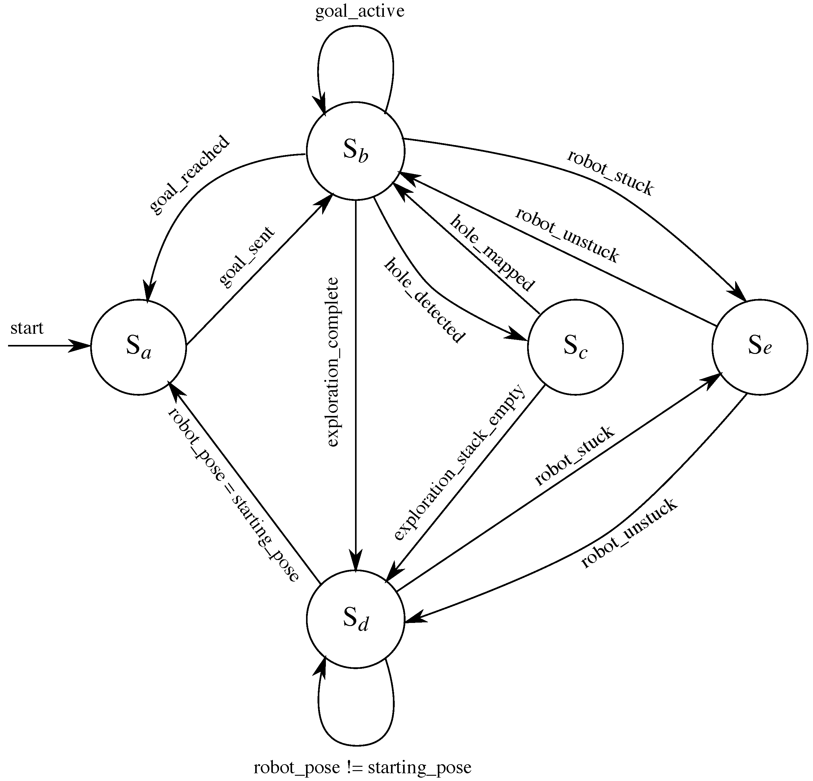
Figure 9.
Navigating a crossroad with the map edgealgorithm.

Figure 10.
Front and side view of the developed robot: (a) robot front view; (b) robot side view.
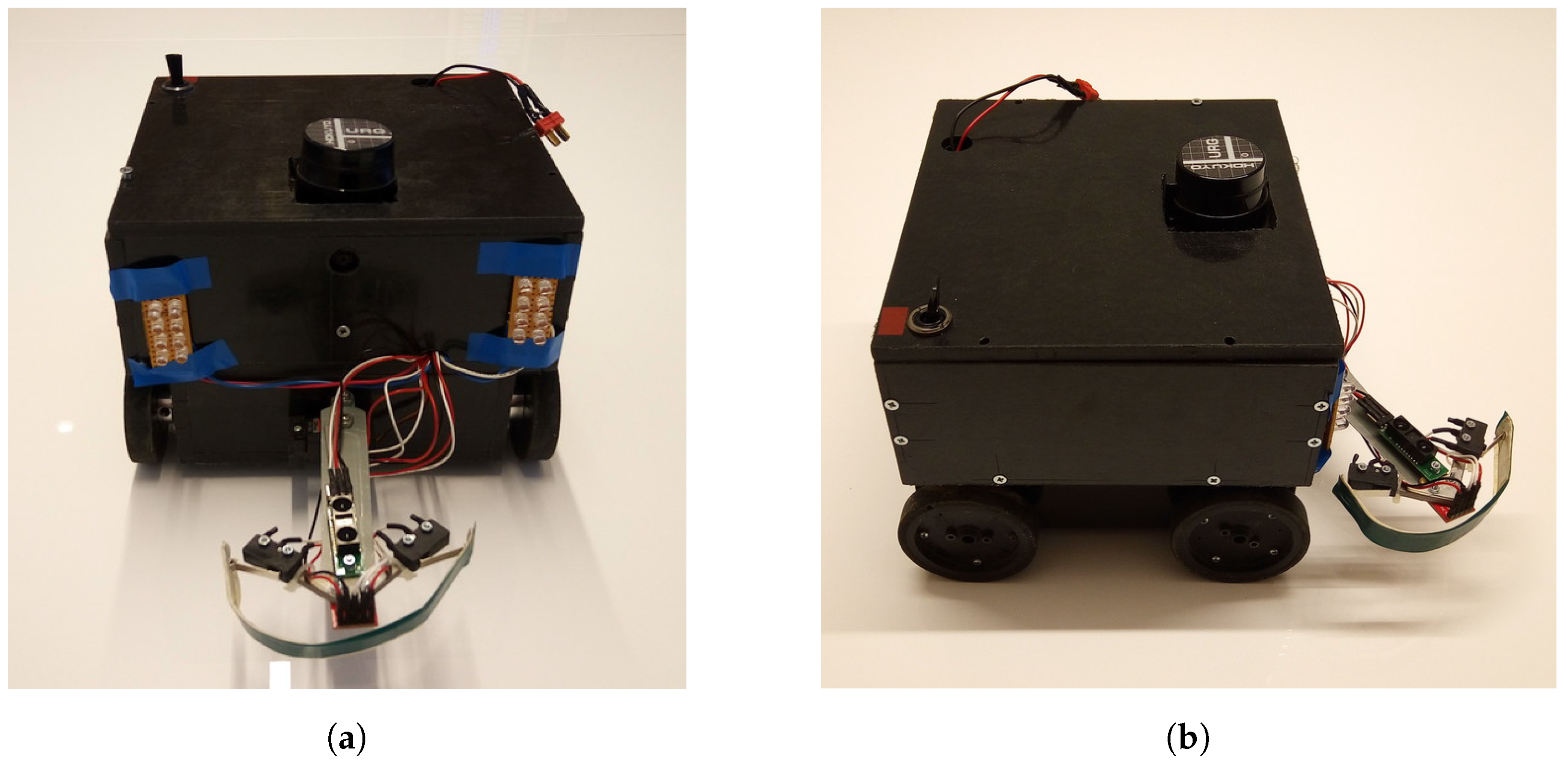
Figure 11.
Exploration and mapping of a simple duct. Both maps—SLAM map and costmap—were generated concurrently: (a) simple duct environment with walls depicted by transparent red barriers; (b) map generated using SLAM by the slam_gmapping node; (c) global costmap generated by the ROS navigation stack.
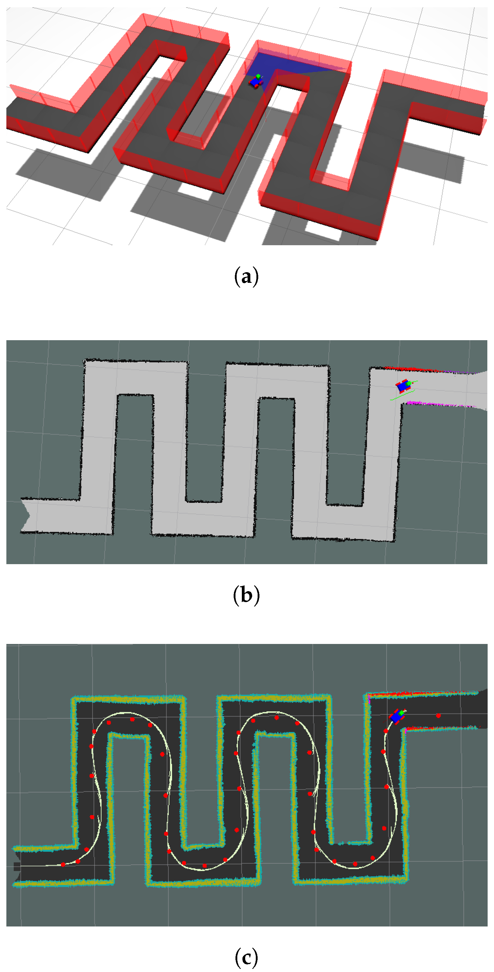
Figure 12.
Exploration and mapping of a duct with dead-ends and branches. Both maps—SLAM map and costmap—were generated concurrently: (a) advanced duct environment with a crossroad and two dead-ends; (b) map generated by the slam_gmapping node; (c) global costmap generated by the navigation stack.
Figure 12.
Exploration and mapping of a duct with dead-ends and branches. Both maps—SLAM map and costmap—were generated concurrently: (a) advanced duct environment with a crossroad and two dead-ends; (b) map generated by the slam_gmapping node; (c) global costmap generated by the navigation stack.
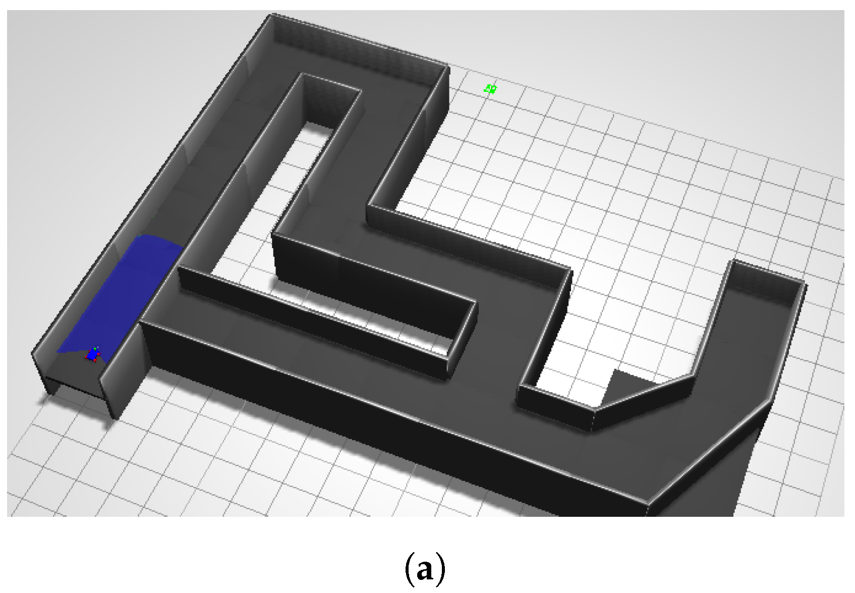

Figure 13.
Errors on goal computation and exploration time dependence on resolution.


Table 1.
ROS nodes and their minimum, maximum and mean processor usage.
| Node Name | CPU Usage (%) | ||
|---|---|---|---|
| Min | Max | Mean | |
| roslaunch | 0.3 | 75.1 | 1.04 |
| rosmaster | 0 | 39.1 | 0.43 |
| rosout | 0 | 5.6 | 1.5 |
| hokuyo_node | 1.3 | 3.3 | 1.98 |
| robot_odom | 0 | 8.6 | 1.69 |
| robot_bumper | 0 | 2.6 | 0.22 |
| robot_tf | 0 | 3.6 | 1.15 |
| twist_mux | 0 | 6.6 | 0.37 |
| logic_node | 1.3 | 7.9 | 1.67 |
| current_sensor | 0 | 4.6 | 0.33 |
| robot_shining | 0.3 | 3.6 | 1.24 |
| ekf_localization | 7.3 | 57.8 | 45.86 |
| move_base | 2.3 | 50.3 | 11.57 |
| servo_motor | 2.6 | 6.5 | 4.65 |
| led_controller | 0 | 2.6 | 0.22 |
| motors_controller | 0 | 23.7 | 0.6 |
| imu_reader | 3.9 | 31.5 | 27.23 |
| ir_short | 4.6 | 7.2 | 6.04 |
| ir_long | 0 | 4.6 | 0.43 |
| ir_2d_nav_node | 4.9 | 26 | 5.85 |
© 2017 by the authors. Licensee MDPI, Basel, Switzerland. This article is an open access article distributed under the terms and conditions of the Creative Commons Attribution (CC BY) license (http://creativecommons.org/licenses/by/4.0/).
Share and Cite
MDPI and ACS Style
Koledoye, M.A.; De Martini, D.; Carvani, M.; Facchinetti, T. Design of a Mobile Robot for Air Ducts Exploration. Robotics 2017, 6, 26. https://doi.org/10.3390/robotics6040026
AMA Style
Koledoye MA, De Martini D, Carvani M, Facchinetti T. Design of a Mobile Robot for Air Ducts Exploration. Robotics. 2017; 6(4):26. https://doi.org/10.3390/robotics6040026
Chicago/Turabian StyleKoledoye, Moses A., Daniele De Martini, Massimo Carvani, and Tullio Facchinetti. 2017. "Design of a Mobile Robot for Air Ducts Exploration" Robotics 6, no. 4: 26. https://doi.org/10.3390/robotics6040026
Note that from the first issue of 2016, this journal uses article numbers instead of page numbers. See further details here.