Teaching Joint-Level Robot Programming with a New Robotics Software Tool

Department of Software Engineering, Florida Gulf Coast University, Fort Myers, FL 33965, USA
*
Author to whom correspondence should be addressed.
Robotics 2017, 6(4), 41; https://doi.org/10.3390/robotics6040041
Submission received: 1 November 2017
/
Revised: 4 December 2017
/
Accepted: 11 December 2017
/
Published: 18 December 2017
Abstract
:With the rising popularity of robotics in our modern world there is an increase in the number of engineering programs that offer the basic Introduction to Robotics course. This common introductory robotics course generally covers the fundamental theory of robotics including robot kinematics, dynamics, differential movements, trajectory planning and basic computer vision algorithms commonly used in the field of robotics. Joint programming, the task of writing a program that directly controls the robot’s joint motors, is an activity that involves robot kinematics, dynamics, and trajectory planning. In this paper, we introduce a new educational robotics tool developed for teaching joint programming. The tool allows the student to write a program in a modified C language that controls the movement of the arm by controlling the velocity of each joint motor. This is a very important activity in the robotics course and leads the student to gain knowledge of how to build a robotic arm controller. Sample assignments are presented for different levels of difficulty.
1. Introduction
Introduction to Robotics is a common introductory robotics course generally covering the fundamental theory of robotics including robot kinematics, dynamics, differential movements, trajectory planning and basic computer vision algorithms commonly used in the field of robotics. Joint programming is a fundamental part of this course and involves a deep understanding of robotics theory including robot kinematics, dynamics, and trajectory planning.
Joint programming is the task of writing a program to directly control the robot’s joint motors as opposed to simply telling the robot’s controller where to move the arm. Ultimately all robotic movements are performed by controlling the input power source to each joint motor.
Trajectory planning activities are a vital part of joint programming and involve navigating the arm considering the impacts of its momentum. The trajectory plan must consider the instantaneous velocity and acceleration limits of each joint motor in order to produce coordinated movements. Traditionally, universities tend to use real industrial robotic arms for this course. However, today, commercially available arms come with a controller that performs this joint programming, which, in fact, constitutes an obstacle in teaching. Students will need to bypass the arm’s included controller to gain direct access to the joint motors in order to perform and learn any joint programming. This is not desirable or possible as the controller includes many safety features that, if overridden, void all warrantees and expose the educational institution to any liability resulting from accidents associated with the controller not being actively in control of the arm. It is unlikely any educational institution will allow such an activity.
On the other hand, small light weight toy arms are sometimes used for this purpose, however, due to their light weight, they cannot accumulate any significant momentum when moving. When their joint motors are turned on or off, they reach their new speed almost instantly with no need to consider acceleration delays. Therefore, they do not possess the dynamic characteristics of an industrial arm. In addition, these toy arms do not allow one to move the joint motors at variable speeds. Without considering momentum and variable speed control, trajectory planning becomes unnecessary as the joint motors are simply turned on at the beginning of the path and off when it arrives at its destination angle. Unfortunately, without the need for trajectory planning, joint programming becomes trivial. Thus, there is unquestionable need for an educational software tool that provides an opportunity to perform joint programming using a virtual arm with user specified dynamics.
An alternative approach, which we pursue, would involve a virtual setting, where all the constraints described above can be modeled. The software tool presented here provides an opportunity to perform joint programming using a virtual arm with user specified dynamics. That is, to properly control the arm, the student will need to consider momentum and acceleration limits to control the speed of the arm rather than just turning on and off the joint motors. This requires the student to implement proper trajectory plans as they learned in the course.
This tool is specifically designed to support teaching and learning essential concepts in an introductory robotics course. The introduction to robotics textbook by Nikku [1] was used to guild the development of this tool. The topics the tool supports are based on the topics covered in this textbook and include forward and inverse kinematics, the Denavit and Hartenberg (DH) parameter and frame placement convention, trajectory planning, robot vision, and joint-level programming.
This paper presents the newly added joint programming capabilities available in the tool. Work needed to develop such capabilities involves creating an interpreter using a newly developed language that is based on the C programming language with MATLAB matrix syntax and capabilities. An LR(1) parser generated using the Yet Another Compiler Compiler (YACC) tool, parses the input source code and produces a parse tree which is then traversed in the process of executing the input program which then has ties to the virtual arm’s joint motors.
Our previous work on various parts of this tool, presented in several publications [1,2,3,4], involved offering a way for the student to perform robotics activities without the need of an actual robotic arm. There exist a number of general purpose robotic simulators both free and commercially available [5,6,7,8]. These tools are used for professional robotics research and related work as well as for educational purposes. The problem with using these general tools for teaching an introductory robotics course is that, first, there is a relatively steep learning curve needed to get sufficiently familiar with the tool before the student can use them for learning robotics. Our tool is specifically designed to allow a student who has never used the tool before to input the specifications of the robotic arm and get to the point where the student can move the links of the robot and adjust the viewing position in less than 5 min.
Second, actual robots are programmed using an included environment that uses a custom scripting language that performs all the inverse kinematics, trajectory planning, and joint programming required for the robot. While this is how real robots are programmed, it does not lend itself to learning introductory robotics since the logic in these preexisting software components is precisely what the student needs to learn how to create. This tool differs from these existing robotic simulation tools in that it is specifically designed to teach this specific course and therefore has a much smoother learning curve and does not do the work itself but rather supports the student while they do the work.
Peter Corke [9,10] has developed a library of MATLAB functions and has made it freely available. This library is very popular but requires the student to write programs in MATLAB. There is no integrated development environment (IDE) associated with the library, so the level of programming is more extensive, and the investment of time needed to learn MATLAB, create the complete program and setup the virtual arm is much greater than using the tool presented here. This level of programming is not always feasible especially at institutions that do not have a software intensive program (for example, the Systems Engineering Program at Texas A&M International University, previous institution of the first author) or in programs where this course is offered only as an elective. As an elective that is not part of a robotics concentration, students are less likely to invest the time needed to appreciate the library from Peter Corke.
Another characteristic of Corke’s toolbox is that the philosophy of learning is different than the philosophy used to design the tool presented here. This is shown in [11], which describes how Corke’s MATLAB toolbox can be used to allow the student to perform basic robotics activities. For example, they use the fkine() function to have the tool compute the forward kinematic equations of the arm provided. The jtraj() and ctraj() functions compute the joint and Cartesian space trajectory path. Our philosophy, however, is that a tool that performs these activities for the student is not as effective as a tool that supports the student in performing these activities. For example, our tool does not perform either of these functions but rather provides a programming platform where the student can program the arm, thus, requiring them to successfully perform the inverse kinematics and compute the trajectory plan. The end result is that the student must perform these activities, such as derive the inverse kinematic equations and compute a trajectory plan and use it in programming the arm. The tool only provides the programming platform that includes the virtual arm. It does provide MATLAB functionality to support the student. For example, it can compute the inverse of a matrix needed in computing polynomial trajectories.
In fact, tools that preform the learning activities themselves rather than support the student in performing them are very common. For example, ref. [12] describes a simulator for mobile robots, where the tool performs the motion planning. The user only enters some parameters that impact the way the tool performs these activities. The authors do claim the tool is to be used by the instructor in class and not to support the student directly. In another example, ref. [13] presents a package of three tools, one of which, Inverse Kinematics Computations (IKC), computes numerical solutions to the inverse kinematic equations. The same tool allows the use of a virtual arm by providing it with a set of DH parameters much the same way it is done in the tool presented here. It also includes a symbolic processor for multiplying the individual transformation matrices to derive a set of forward kinematic equations.
All of these tools are useful for students that will take many robotics courses and will eventually need to work with very complex arms where these activities may be too difficult to do without such tools, however, in an introductory robotics course, the present authors believe it is better to provide a simple arm where the students can perform these activities themselves.
There is another group of software tools that are more aimed at supporting the student to learn. In [14], the authors present a tool that renders the arm given its D-H parameters. It is a web-based tool that one needs to interface via a TCP/IP socket connection. Once the arm is rendered the user can move the eye and see the 3D arm from different views. The presented tool also accepts its arm model by allowing the user to enter its D-H parameters and renders the kinematically correct arm using 3D graphics, see [1]. It also allows the user to move the eye and view the arm from different angles. In [15] they present a tool that supports learning concepts related to forward and inverse kinematic equations and specifically deals with joint and Cartesian workspaces. The tool produces a reachability plot in a 3D Cartesian workspace by varying the theta angles. The presented tool supports learning forward and inverse kinematic equations by rendering the arm and allowing the user to move the virtual arm’s joints individually using sliders. In [16] the authors present a tool that supports learning forward and inverse kinematic equations using quaternion algebra. Quaternion numbers are like complex numbers but work in four dimensions. The presented tool does not support the use of quaternion algebra and this topic is not found in [1] either. Their tool does have some animated movement they refer to as trajectory planning but the user is not at all involved in the design of the trajectories only to specify the type of movement the tool is to use. The tool is not designed to support learning trajectory planning but rather is used as a way to support quaternion algebraic equations. In contrast to the presented tool, all of these tools support forward and inverse kinematic equations and the relationship between Cartesian and joint workspaces. They do not provide any support for learning joint-level programming or even trajectory planning. From the software point of view, all of the fundamental mathematical concepts including forward and inverse kinematic equations, transformation matrices, and the math involved in path planning are to support the ultimate goal of joint-level programming yet there is no known tool that directly supports this activity. Consider learning how to program using the Java programming language and not having access to a Java compiler. Many institutions use real robotic arms for this course however, using an actual industrial robotic arm will not allow student to execute joint-level programs either since, for safety reasons as explained earlier in this paper, their manufacturers do not allow direct access to its joint motors.
In this paper, we introduce a new complex component of our tool, specifically designed for an introductory robotics course, which offers the ability to allow programming the virtual arm at the joint level. That is, the tool allows the student to write a program in a modified C language that controls the movement of the arm by directly controlling the velocity of each joint motor. With this tool, the course instructor can assign joint-level programming assignments since the tool can compile and run these programs. This is a very important activity in the course and leads the student to gain knowledge of how to build a robotic arm controller.
2. Materials and Methods
2.1. Educational Guidance for Tool Design
When designing the tool for educational use, the focus has to be on addressing the acquisition of knowledge by the students and having them acquire respective professional competencies. In engineering, the high-level guidelines are expressed in ABET [17] criteria (3a) through (3k), of which the following are suitable for the introductory robotics course:
- (3a) an ability to apply knowledge of mathematics, science and engineering
- (3b) an ability to design and conduct experiments, as well as to analyze and interpret data
- (3c) an ability to design a system, component or process
- (3e) an ability to identify, formulate and solve engineering problems
- (3k) an ability to use the techniques, skills and modern engineering tools necessary for engineering practice.
In addition, for practical purposes, the focus of this tool is for the students to achieve a high return on investment. This leads to a tool designed to allow for maximum acquisition of knowledge, with a minimum amount of overhead time to learn how to use the tool and to setup the environment. The software’s goal is to model any robotic arm that one can model using standard DH parameters. The virtual arm is created by simply entering the DH parameters for the arm along with the range and acceleration limits for each link. This includes 4 numbers per joint plus an additional three for the range and acceleration limits, if the default values are not desired.
Taking all this into account, the joint programming features of this tool are designed to support the students learning joint programming and related theory. The specific learning outcomes the joint programming feature of the tool helps address, mapped on the ABET criteria, are as follows. After completion of the course the student will be able to:
- Produce a smooth trajectory for the arm (Criterion (3k)).
- Effectively use inverse kinematic equations to determine the joint angles given Cartesian coordinates (Criterion (3a)).
- Produce a program to control the arm by directly controlling each joint’s velocity (Criterion (3c) and (3e)).
- Effectively produce a program to move the arm through several points to complete a complex path using trajectory planning, inverse kinematics equations, and joint programming (Criterion (3b)).
2.2. The Software Tool
2.2.1. The Software Architecture
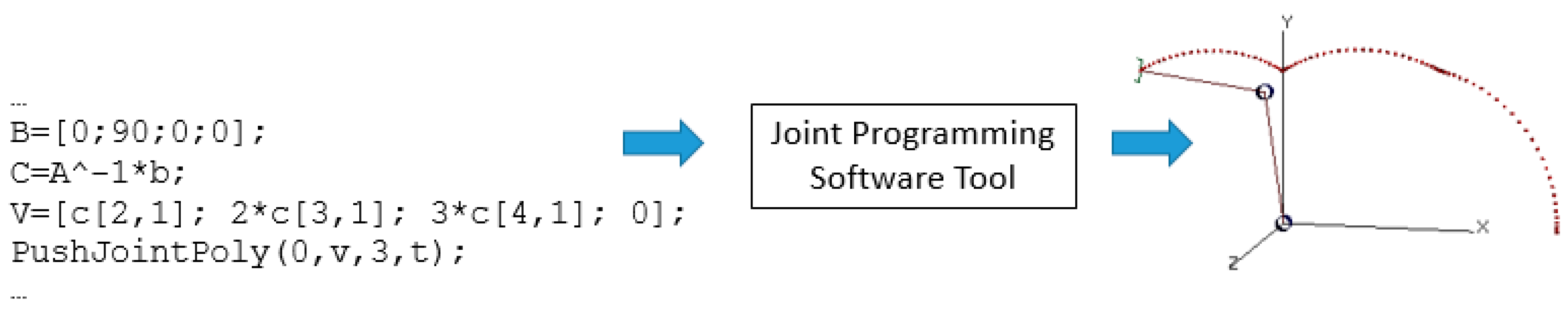
The presented part of the software tool is designed to allow the student to practice moving the arm by having their program control the instantaneous velocity of each joint. In Figure 1, the tool takes, as input, source code written by the student and produces a rendering of the virtual arm that moves in response to the execution of this source code. Joint programming means that the source code entered by the student can only move the arm by providing instantaneous desired velocities at each moment and for each joint.
Figure 2 shows how the user interacts with the tool. The user can enter a model of the arm by specifying the Denavit-Hartenberg parameters of the arm along with the range of movement and a maximum acceleration for each joint, see Figure 3. Once the model is entered the user can move the arm manually using the sliders and move the position of the eye in 3D, see Figure 4. This can be used to verify the model is correct and to position the arm in some initial position. For joint programming, the student can then enter their program using the C/MATLAB language designed specifically for this tool. Once the source code is complete the user can run the program and, if the code is bug free, can view the virtual arm move. The source code must include an instruction to start the simulation and to produce the movement plots if the user desires.
2.2.2. Implementation
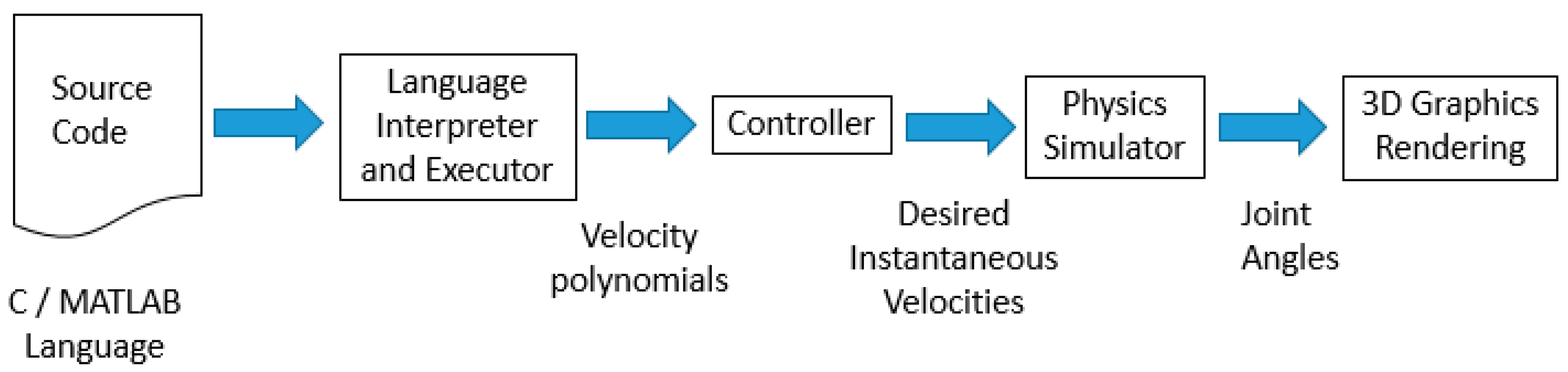
The user-entered program must provide each joint motor an instantaneous desired velocity for each time period during the duration of the movement. The system consists of a language interpreter/executor, controller, the simulation engine that models the physics of the arm, and the 3D rendering of the arm and its motion, see Figure 5. The components of the tool model the components in a commercial robotic arm which includes two components, the physical arm, modeled by the simulation engine and the 3D rendering components and the controller modeled by the controller component and the interpreter and executor executing the student supplied source code. The controller included in a commercial product performs all the joint-level programming internally.
In our tool, the controller accepts a velocity polynomial that it uses to compute the instantaneous desired velocity given the current time offset from the beginning of the trajectory. The simulation engine then uses these desired velocities along with the model of the arm to produce physically accurate arm movements. We will first discuss the left half of the system shown in Figure 5, the controlling side, which includes from the source code to the controller. After we will discuss the right half, the physical side, which includes the simulation engine and 3D rendering.
The controlling side of the tool shown in Figure 6, consists of a language parser that accepts source code written in the dedicated C/MATLAB language then produces a parse tree representing this code. The parse tree is a recursive structure in that every subtree is itself a parse tree. The executor then traverses this parse tree using a recursive algorithm executing the statements in real time. The program is never compiled since it is executed by the robotics tool and not directly by the computer. During execution, the student’s program calls interface functions that provide the controller with a list of speed polynomials for each joint. Each polynomial is valid for a specific time interval and therefore the controller can receive several polynomials per joint. The controller maintains a queue of polynomials for each joint. During execution of the parse tree, every time the simulation engine requests an instantaneous velocity for the current time, the controller computes it using the current polynomial. If the polynomial is no longer valid, it removes the next polynomial from the joint’s queue and continues with that one. Once there are no more polynomials for a given joint, the controller returns 0 as the desired velocity for that joint.
The parser was created using Yet Another Compiler Compiler (YACC), an old tool that is still the standard. YACC accepts a context free grammar expressed in Backus–Naur form, (BNF), as its input and generates a Look-Ahead-Left-Right, LALR(1) parser. This is a type of shift-reduce parser that performs a reduction once it has seen sufficient tokens to reduce using a production rule from the context free language. During this reduction, the parser calls the expression tree builder and passes it the tokens involve in the reduction. These tokens are removed from the top of the stack. The tree builder then creates a subtree using these tokens and passes the subtree back to the parser where it then pushes it onto the top of the stack. This recursive method will eventually lead to the stack only having the root of the parse tree which can then be removed and passed to the executor for real time execution.
The parse tree is not a legal tree in that is includes many linked lists as well. For example, the root of the tree is actually a linked list of functions with one of them named “void main(…)”. The body of a block, such as the body of a function, is also a linked list of statements. The code interpreter starts at the top of the tree, searches for the function called “main” and executes that function. It traverses the tree in the proper order dictated by the nodes of the tree until the program reaches the end of the body of function main(). At this time the interpreter stops execution. The arm may still be moving if the user program terminates before the arm reaches its destination.
At the other side of the tool, see Figure 7, the physical side, the simulation engine uses the instantaneous desired velocities to determine the arm’s movement based on the proper system dynamics. The virtual arm can only be moved by properly controlling its joint motors much the same way a physical arm is controlled.
The simulation engine is tied to a periodic interrupt that executes 10 times per second. During each interrupt cycle the engine request the controller for the next instantaneous desired velocity for each joint. The algorithm to compute the new position for a single joint follows below. Table 1 shows the symbols used in the equations used in the algorithm. The simulation engine executes this algorithm for each joint. It also checks to see that the movement did not trip a limit switch. If it did the simulation stops and a message pops on the screen over the arm rendering. The student must manually move the arm back to a valid position away from any limit switch before continuing any activities.
Step 1: Request the next desired velocity, , from the controller.
Step 2: determine the new acceleration that will reach the desired velocity.
Step 3: Limit the acceleration to its negative and positive maximums
if (a > MaxA)
a = MaxA
else if (a < −MaxA)
a = −MaxA
a = MaxA
else if (a < −MaxA)
a = −MaxA
Step 4: Save the current velocity.
Step 5: Compute new velocity.
Step 6: Compute new position.
Step 7: Render the arm in its new position.
The algorithm above executes 10 times per second for each joint. Once it executes, it updates a flag that tells the arm rendering component to render the arm in its new position. At 10 times per second, the arm appears to move following a smooth trajectory.
2.2.3. The Programming Language
The developed language is based on the standard C language but includes some matrix capabilities and syntax similar to that of MATLAB. The language does not include the complete C language but rather only a subset consisting of the most common structures. For example, it does not include the “switch” structure but does include the “if-else” structure. Table 2 shows the set of control structures, data types, and legal operators included in the language. The syntax follows the standard C language syntax and MATLAB syntax for the definition, multiplication, addition, subtraction and inversion of matrices. We chose to base the language in C rather than in MATLAB since C is a more general purpose language. In comparison the MATLAB, it is more likely that a student will already know how to program in C or will benefit from learning it. For example, in MATLAB variables do not need to be declared before being used. For a student that just learned several high-level languages such as Java, C, and C++, and is not yet comfortable with the syntax, this can lead to bad habits such as forgetting to declare variables.
The language supports functions using the C syntax but it does not implement pass-by-reference or even simulated-pass-by-reference as C does since pointer operators are not implemented either. However, functions can return all data types including matrices.
Example 1 shows the code based on the C language but consisting of MATLAB syntax for the matrix operations. Note data type “matrix” is a type native to this language not part of C or MATLAB. Example 2 shows a simple recursive function.
Example 1.
Consider the following system of equations.
Figure 8a shows the program that will solve the system of equations and display the solution. Note the program is written in the C language except for the matrix initializations, inversion and multiplications which are written using MATLAB syntax. The matrix type is an addition to the language as in MATLAB, variables are not declared as they are in C. Figure 8b shows the output of the program execution.
2.2.4. Program Interface Functions
In order to allow the user’s program to move the virtual arm, it needs to interface to the simulation engine by calling specific functions. To model an actual arm, we chose to have the program move the arm by controlling the instantaneous velocity of each joint motor. It was chosen to have the simulation engine receive a velocity polynomial for each motor as opposed to an acceleration or position polynomial.
In an actual physical arm, each joint motor needs a power setting to move. A typical electric motor is controlled by regulating its voltage source. To make interfacing simple, we assume the motors receive a velocity setting as their input. It is common for servomotors, a type of electric motor used in robotics, to expect a velocity setting as their input. When the velocity input changes, it uses the difference between the current and desired velocity coupled with its maximum acceleration limit to determine the change in velocity over time. This maximum acceleration is found in the arm’s model provided by the user. The PushJointPoly(.) function is used to provide the simulation engine with a velocity polynomial. Polynomials are represented as a column vector of coefficients. Example if we have
then we represent the polynomial with
The tool has a periodic interrupt service that executes 10 times per second. During this interrupt, it evaluates every joint polynomial to determine each motor’s desired velocity for the next period and gives this velocity to the module that models the physics of the arm. The velocity will change over time within the constraints set by the maximum accelerations. Once every joint has received its polynomial, the user program must tell the simulator when to stop simulating by calling the StopTimerAt (.) following. Finally, the user program must start the simulation by starting the timer interrupt service. This is done by calling the StartTimer (.) function.
2.2.5. The Simulation
The simulation engine moves the arm based on the velocity each joint has. A parodic interrupt that occurs ten times per second advances the movement of each joint. It first determines if the velocity needs to be changed then it uses this velocity and the joint’s current position to determine the joints new position. The velocity changes when the desired velocity is different than the current velocity. Considering the maximum acceleration, it determines how much the velocity can change in a tenth of a second and only changes the velocity by that amount. It performs this routine for each joint. Once all the joints have been moved, the arm is erased and rendered again in its new position. The rendering of the arm grabs the current position for each joint and using the forward kinematic equations, it determines the precise location of every link in the arm. The tool computes the forward kinematic equations using the D-H parameters in the arm’s model.
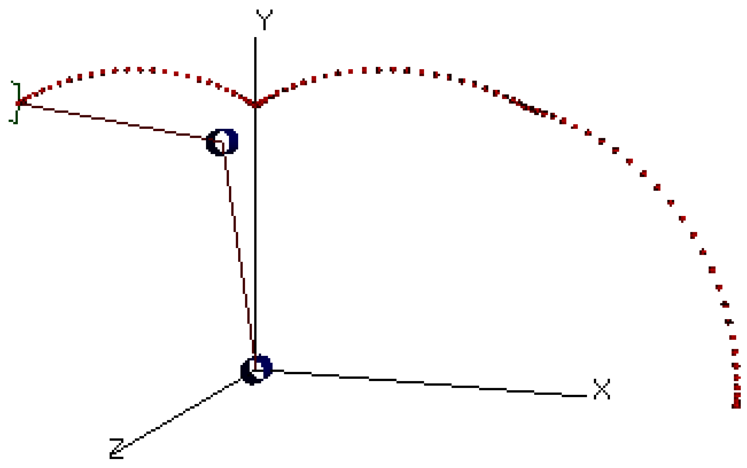
To record the movements of the arm, a trace feature was added. The user can turn on this feature and as the arm moves, it draws dots at the current location of the hand. Since the dots are drawn at even time intervals, the spacing between the dots provide information to the hand’s velocity. A faster moving hand results in the dots spaced apart with greater distance.
The simulation also produces plots for the position, velocity, and acceleration of each joint. The plots are displayed in the tool and MATLAB “m” files with this data are generated as well. This allows the user to plot the data using MATLAB which has a richer set of plotting capabilities. The plots allow the student to produce a static image of the movement so that they can turn it in for grading or include it in a report.
2.3. Student Assignment Problems
The following is a list of assignments the students can perform using this tool’s joint programming features along with their solutions. It is presented to show the type of assignments that can be given using this tool. The level of complexity of the assignment depends of the student’s programming skills, the time the students wishes to devote to the assignment, and the complexity of the task itself.
2.3.1. Example Assignment 1: A Simple Trajectory
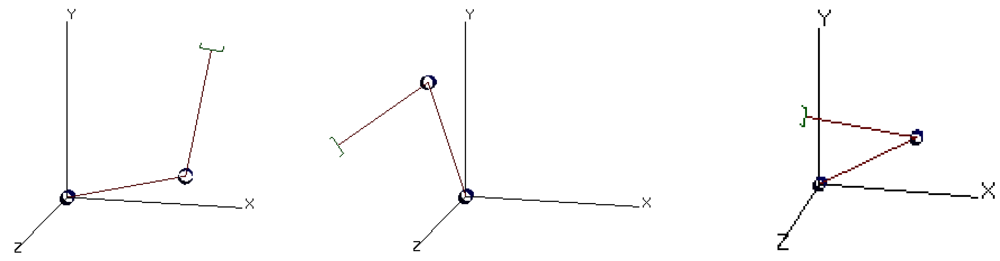
Using the two link planar arm shown in Figure 10, we want to create a trajectory to move the arm from the position shown in Figure 11a to the position shown in Figure 11b in 3 s. The arm is to start and stop with no velocity. Note the arm’s start position is at angles 0° and 180° for joints 1 and 2 respectively and its end position is at angles 90° and 0°. Use a polynomial trajectory for each joint. Use best practices in programming and make your program easily modifiable to solve similar problems with different start and end angles and duration.
Solution:
Step 1: Define the problem mathematically. We want joint 1 to go from 0 to 90° and joint 2 from 180 to 0° in 3 s. In addition, we want the acceleration to be 0 initially and at the end of the trajectory as well. We use the function to represent the joint angle function for joint j at time t that outputs angle, , in degrees. We define the constraints as shown in Table 3. The task is to find and so that we can supply their derivatives to the joint motors to move the arm as desired.
Step 2: Determine the order of the polynomial. Each joint is controlled independently and therefore we need a polynomial for each of the two joints. Since we have 4 constraints per joint, we can use to use a 3rd order polynomial for the position.
Since some constraints are on the velocity of , we can differentiate to get
Step 3: Setup the system of equations. We have the following system of equations:
Putting into matrix form we have:
or
where
Step 3: Solve the system and compute the constants. We need to find . At this time the student may use a matrix software such as MATLAB to compute the coefficients of the polynomials and then enter them into the program which will send them to the joint motors. However, since the programming language includes MATLAB type matrix capabilities, the student can have their program solve the system of equations and take the polynomials directly from the result.
Step 4: Write the program to move the arm. Each joint motor needs a velocity function, , so the student needs to differentiate which can easily be done by simply shifting the elements in the vector and multiplying them by increasing constants. For example, if represents , then represents . The following line of code differentiates the polynomial. The vector v is the derivative of vector c.
v = [c[2,1]; 2*c[3,1]; 3*c[4,1]; 0];
The complete program shown in the tool’s programming windows is shown Figure 12. When the program executes, the virtual arm moves in real time. The student will be able to see this movement. However, to record this movement, the trace feature was turn on before running the program. Figure 13 shows the output trace. Note a dot is displayed at the location of the hand at even time intervals. As the arm moves faster the dots are displayed farther apart from each other. The density of the dots gives information to the speed of the hand. The tool also produces a plot of the position, velocity and acceleration of the hand as it moves. Figure 14a,b shows the plot for the two joints. The data for the plot start when the timer starts and ends when the timer ends so it only includes the time specified in the program. The timer starts when the StartTimer ( ) function executes and ends when the movement polynomial queue get empty. In addition, the tool produces a MATLAB “m” file with the same data to allow the student to use MATLAB’s more advanced plotting features.
2.3.2. Example Assignment 2: A Multi-Trajectory Path
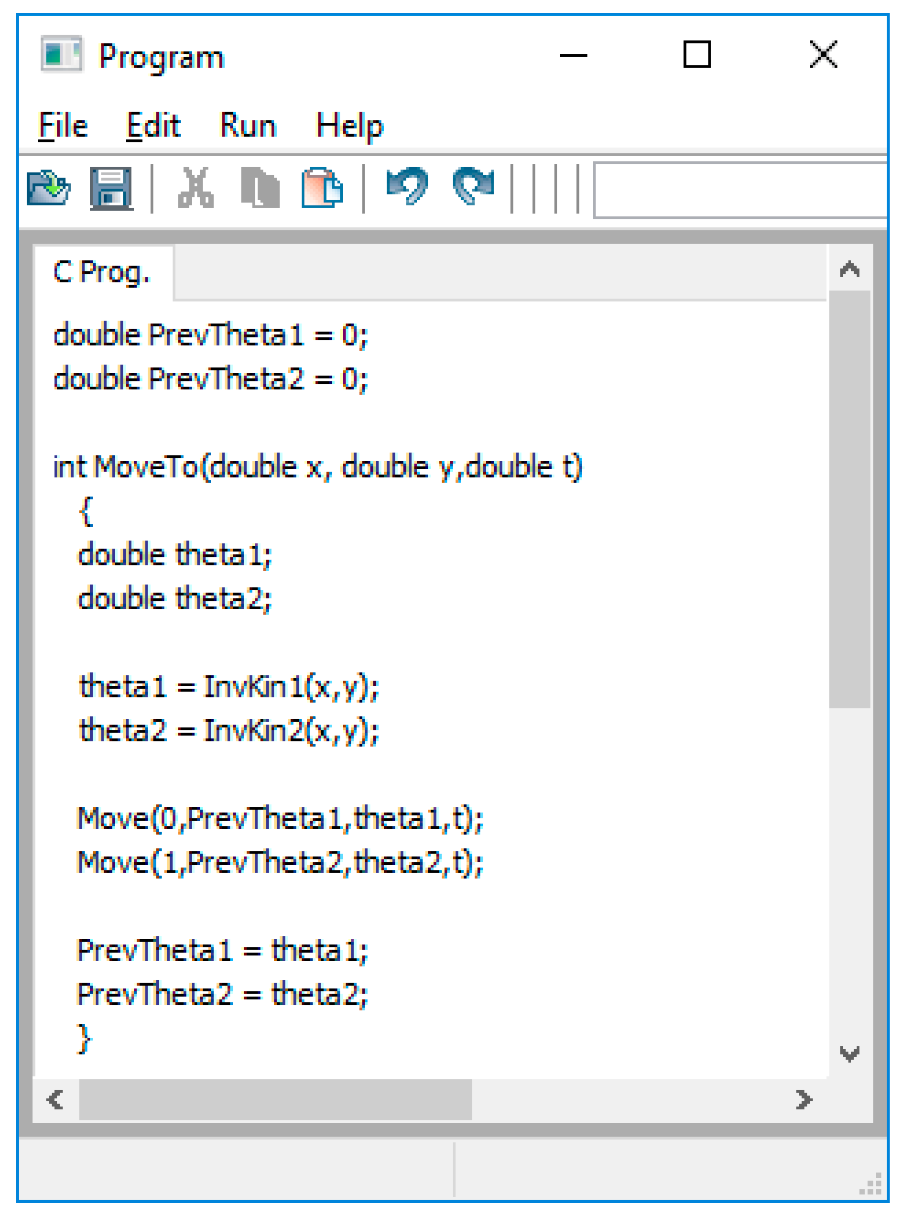
In this example the student has to create several functions as follows. The first is to compute the velocity vector given the initial and final theta and the duration, assuming the initial and final velocity is 0. Next, the student is to create a function that determines the joint angles given the x and y coordinates using the inverse kinematics equations for the arm, and finally they are to create a function that given the next x–y coordinate to move to, it instructs the arm to move to that location. This function must remember the location that it is at. Note this assignment requires the student to determine a set of inverse kinematic equations for the arm.
Computing the inverse kinematic equations is an important topic in this course. Without a tool, the student will only be able to find a set of inverse kinematic equations and perhaps turn it in as homework. With the joint programming capability of the tool, they can implement the inverse kinematic equations they calculated and test it with the arm.
Solution:
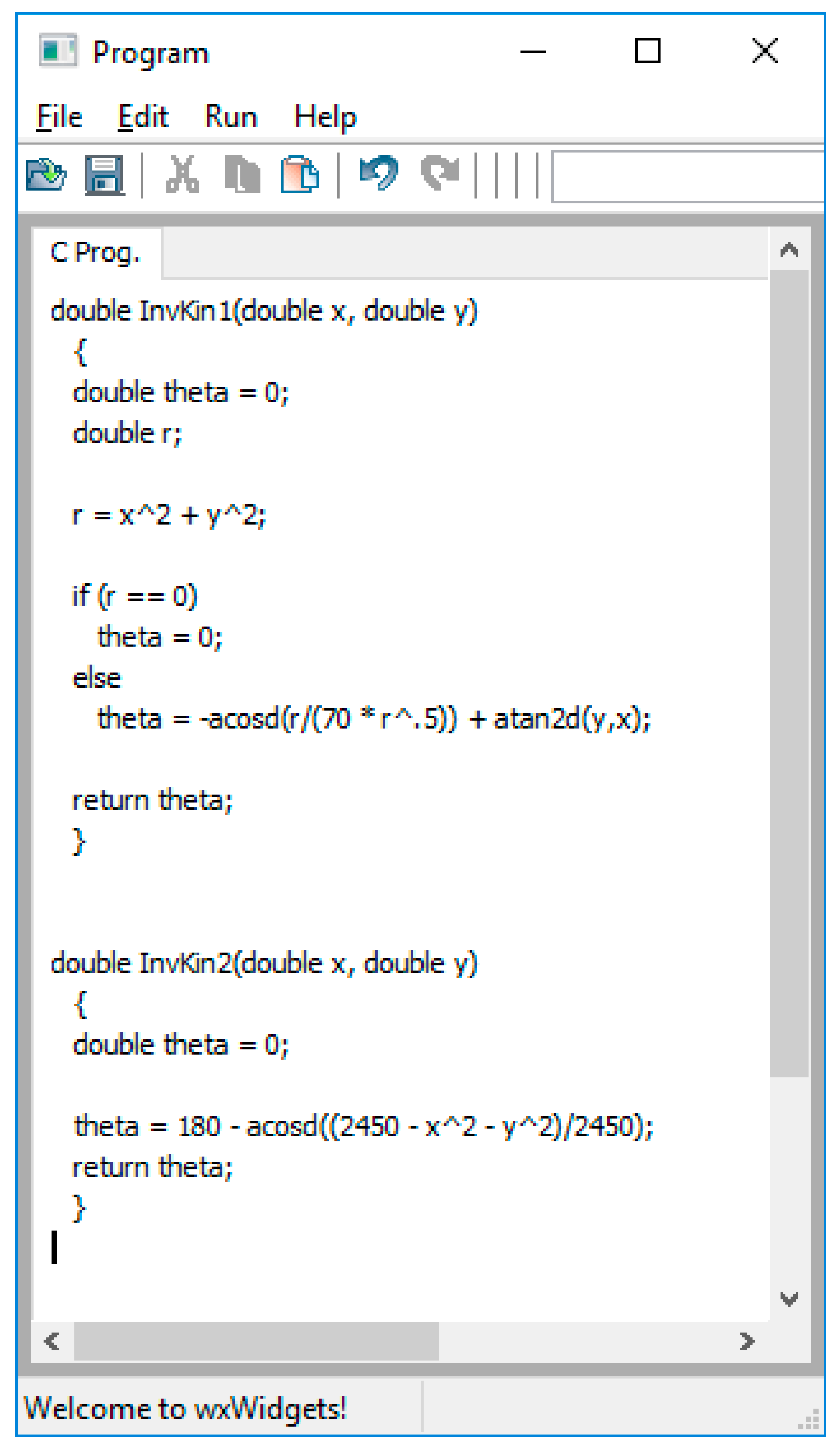
For this arm the inverse kinematic equations are shown below. The link length constants and are 35 each.
The function to compute the velocity vector given the initial and final velocity and the duration is shown in Figure 15. The function to compute the inverse kinematic equations for both theta 1 and theta 2 is shown in Figure 16, and the function that moves the arm given the desired Cartesian coordinates is shown in Figure 17.
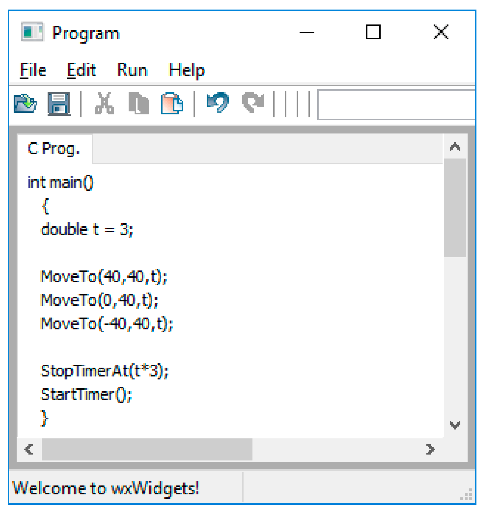
The functions are to be called to move to three different points. In this example solution the arm is programmed to move to point (40, 40) then to (0, 40) and finally to (−40, 40). The main program is shown in Figure 18 and the output trace is shown in Figure 19.
Please notice that the number of lines of code is relatively small and yet the exercise covers three areas of robotics theory, path planning, inverse kinematics, and joint programming. In addition, it allows the student to learn how all this theory is put together to produce a complete robot control program.
3. Results
The tool was used to support “Special Topics: Introduction to Robotics” in the spring semester of 2017. The students used the tool throughout the semester to help them with their homework. For the final project the students were given the D-H parameters to an arm that can hold a pen and write on a sheet of paper. The pen draws when the tip is close to the paper. The assignment was to have the students control the arm to draw the first letter of their name across the top of the paper. They could only control the arm by directly controlling each joint motor’s velocity.
The students were given a survey at the end of the semester to evaluate the use of the tool for this assignment. The survey asked students to rank each question by indicating one of the following scales, Strongly Agree, Agree, Neutral, Disagree, or Strongly Disagree. The questions asked about the three main areas of robotics theory and how all this theory plays a role in the control of a robot.
The class had 38 students registered. Thirty-one of them completed the survey. A weighted average was computed for each of the 14 questions using the scale in Table 4. This includes converting each response to a scale using Table 4 then computing an average.
For example: suppose 3 students responded to a question with the responses being “strongly agree”, “agree”, and “disagree”. Then the average will be which lies between neutral and agree.
The results are shown in Table 5 below.
The average of all the 14 averages is 3.01 which indicates that the students tend to agree with the statements in the survey. The survey also revealed that the tool can improve its ease of use. Specifically related to joint-level programming, the compiler can improve its feedback when a user’s program does not run properly. The error messages produced now are not clear and will be improved.
This course was also taught during the spring of 2016 and the tool was used but did not support joint-level programming at that time. Exam number 2 in both semesters primarily covers trajectory planning. While neither semester had a question asking the student to write a joint-level program, both had an equal amount of questions asking to produce trajectory plans. To write a working joint-level program, the student must master trajectory planning since that is the main part of the joint program. In 2016 the average on Test 2 was 83.2 while in 2017 it was 89.3. The authors believe these Test 2 grades and the survey results indicate the tool was effective in helping the students learn the material in the course and specifically the joint-level programming material.
4. Discussion
Joint-level programming ties together several critical parts of robotic theory including forward and inverse kinematics, transformation matrices, and the math involved in trajectory planning to produce the ultimate result of being able to control the arm directly by continuously giving a power setting to each joint motor as it moves. To produce a program that successfully controls the arm at the joint level, the student must find the forward and inverse kinematic equations and produce the trajectory planning in addition to the actual production of the source code. Joint programming is the best way to learn these components because they tie all these parts together and show the student how they work together and why each is needed. For a student to master joint-level programming, the tool must accept their source code and compile and run it providing feedback on its execution. Otherwise it is like learning how to program without the use of a compiler.
Two example assignments were presented along with their solutions. It should be noted that while neither assignment involves extensive programming, the learning is very rich. The student must master all the components mentioned above to produce a working program. The survey results show that the students rated the tool’s ability to help them learn the relevant material at a mix between strongly agree and agree. The grade comparison between two semesters where one used the tool to support joint-level programming and the other did not, show that the students’ performance using the tool was better by about 6% on the corresponding exam.
5. Conclusions
The presented tool provides a resource where students can program the movement of the arm by controlling the joint motors directly. It is also an activity that ties together many of the fundamental mathematical concepts covered in the Introduction to Robotics course. To support such activities, the software tool contains a virtual arm, a simulation engine modeling the physics of the arm, and a compiler that compiles and runs the students’ programs providing feedback using the movements of the virtual arm.
A future extension will tie in the robotic vision component of the tool. The tool’s virtual environment will have a camera looking down at the robot’s workspace. The user will be allowed to place obstacles in the workspace. Then the arm can be programed to see, identify the object, locate the object’s position and orientation, and finally control the arm to grab and pick up the object. An interface function will be added to the joint-level programming language to input an image from the camera into the program where the student can then call the appropriate vision functions to perform the required movements.
As an extension, the camera may be attached to the arm and the image captured will move as the arm moves. The student can use this image to navigate the arm using visual feedback, a topic beyond the scope of an introductory robotics course.
However, before these future enhancements are added, the graphical user interface in the IDE needs to be improved and the tool needs to be made easier to use. Each time the tool is used in the course, feedback information is gathered from the students as to the characteristics they liked and disliked the most as well as any suggestions for improvements. During the 2017 semester that the tool’s joint-level programming part was first used, the tool went through extensive changes as we tried to fix and add features in real time. As with most software, it is an iterative process that never ends.
Acknowledgments
This research was supported by the Department of Software Engineering at Florida Gulf Coast University. Funds from this source was used to cover the publication cost.
Author Contributions
F.G. conceived the tool and was the primary architect and programmer developing the software tool. He used the tool in his Introduction to Robotics class and wrote parts of the paper. J.Z. made significant contributions to the paper and designed the student survey and the assessment methods used in the assessment of the tool.
Conflicts of Interest
The authors declare no conflict of interest.
References
- Niku, S. Introduction to Robotics: Analysis, Control, Applications, 2nd ed.; Wiley: New York, NY, USA, 2011; ISBN 978-0-470-60446-5. [Google Scholar]
- Gonzalez, F.; Zalewski, J.; Pinzon, G. An Educational Tool to Support Introductory Robotics Courses. In Proceedings of the 122nd ASEE Annual Conference, Seattle, WA, USA, 14–17 June 2015. Paper No. 13128. [Google Scholar]
- Gonzalez, F.; Zalewski, J. A New Robotics Educational System for Teaching Advanced Engineering Concepts to K-12 students. Comput. Educ. J. 2016, 26, 61–73. [Google Scholar]
- Gonzalez, F.; Zalewski, J. An Educational Tool to Support Learning Robot Vision. Trans. Tech. STEM Educ. 2016, 1, 60–82. [Google Scholar]
- GAZEBO Robot Simulation Software. Available online: http://www.gazebosim.org (accessed on 11 February 2016).
- Robologix Logic Design Inc. Available online: http://www.robologix.com (accessed on 23 October 2016).
- Webots 7 by Cyberbotics Professional Mobile Robot Simulator. Available online: http://www.cyberbotics.com (accessed on 16 December 2017).
- Robotics Developer Studio. Available online: http://msdn.microsoft.com/en-us/library/bb648760.aspx (accessed on 10 December 2016).
- Peter Corke MATLAB Tool Box for Robotics. Available online: http://www.petercorke.com/RVC/top/toolboxes/ (accessed on 15 September 2016).
- Corke, P. MATLAB toolboxes: Robotics and vision for students and teachers. IEEE Robot. Autom. Mag. 2007, 14. [Google Scholar] [CrossRef] [Green Version]
- Tijani, I.B. Teaching Fundamental Concepts in Robotics Technology using MATLAB Toolboxes. In Proceedings of the 2016 Global Engineering Education Conference (EDUCON), Abu Dhabi, United Arab Emirates, 10–13 April 2016. [Google Scholar]
- Gonzalez, R.; Mahulea, C.; Kloetzer, M. A MATLAB-based Interactive Simulator for Mobile Robotics. In Proceedings of the 2015 IEEE International Conference on Automation Science and Engineering (SACE), Gothenburg, Sweden, 24–28 August 2015. [Google Scholar]
- Manseur, R. Software—Aided Robotics Education and Design. In Proceedings of the 2016 Global Engineering Education Conference (EDUCON), Abu Dhabi, United Arab Emirates, 10–13 2016. [Google Scholar]
- Robinette, M.F.; Manseur, R. ROBOT-DRAW, an Internet-Based Visualization Tool for Robotics Education. IEEE Trans. Educ. 2001, 44, 29–34. [Google Scholar] [CrossRef]
- Mateo Sanguino, T.J.; Andujar Marquez, J.M. Simulation Tool for Teaching and Learning 3D Kinematics Workspaces of Serial Robotic Arms with up to 5-DOF. Comput. Appl. Eng. Educ. 2010, 20, 750–761. [Google Scholar] [CrossRef]
- Cakir, M.; Butun, E. An Educational Tool for 6-DOF Industrial Robots with Quaternion Algebra. Comput. Appl. Eng. Educ. 2007, 15, 143–154. [Google Scholar] [CrossRef]
- ABET Engineering Accreditation Commission, Criteria for Accrediting Engineering Programs; 2016–2017 Accreditation Cycle; ABET: Baltimore, MD, USA, 16 October 2015.
Figure 1.
Overview of the system.

Figure 2.
Use case diagram for joint programming component.
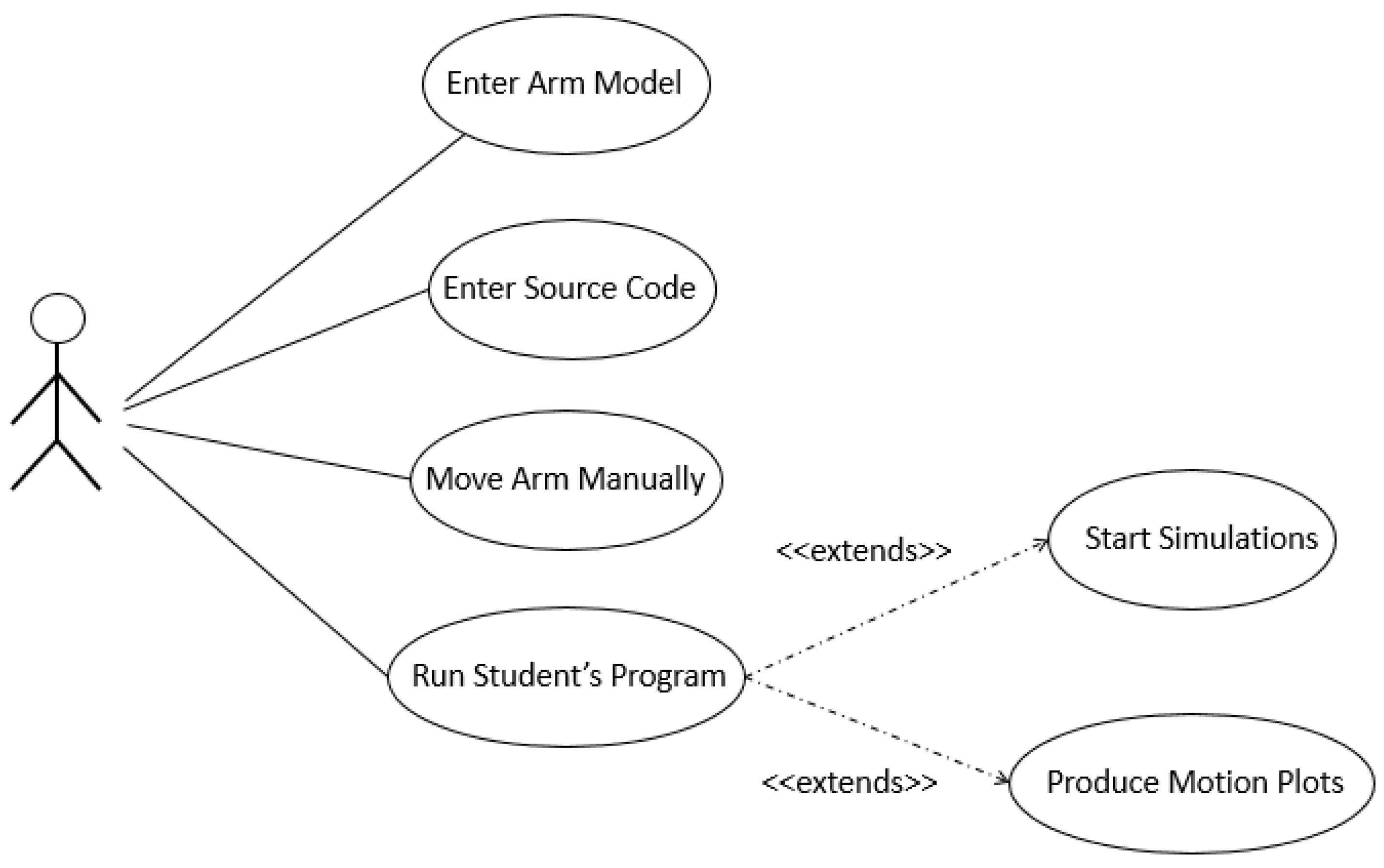
Figure 3.
The window used to enter the model of the arm. The model is specified by each link’s D-H parameters, range limits and acceleration limit.
Figure 3.
The window used to enter the model of the arm. The model is specified by each link’s D-H parameters, range limits and acceleration limit.

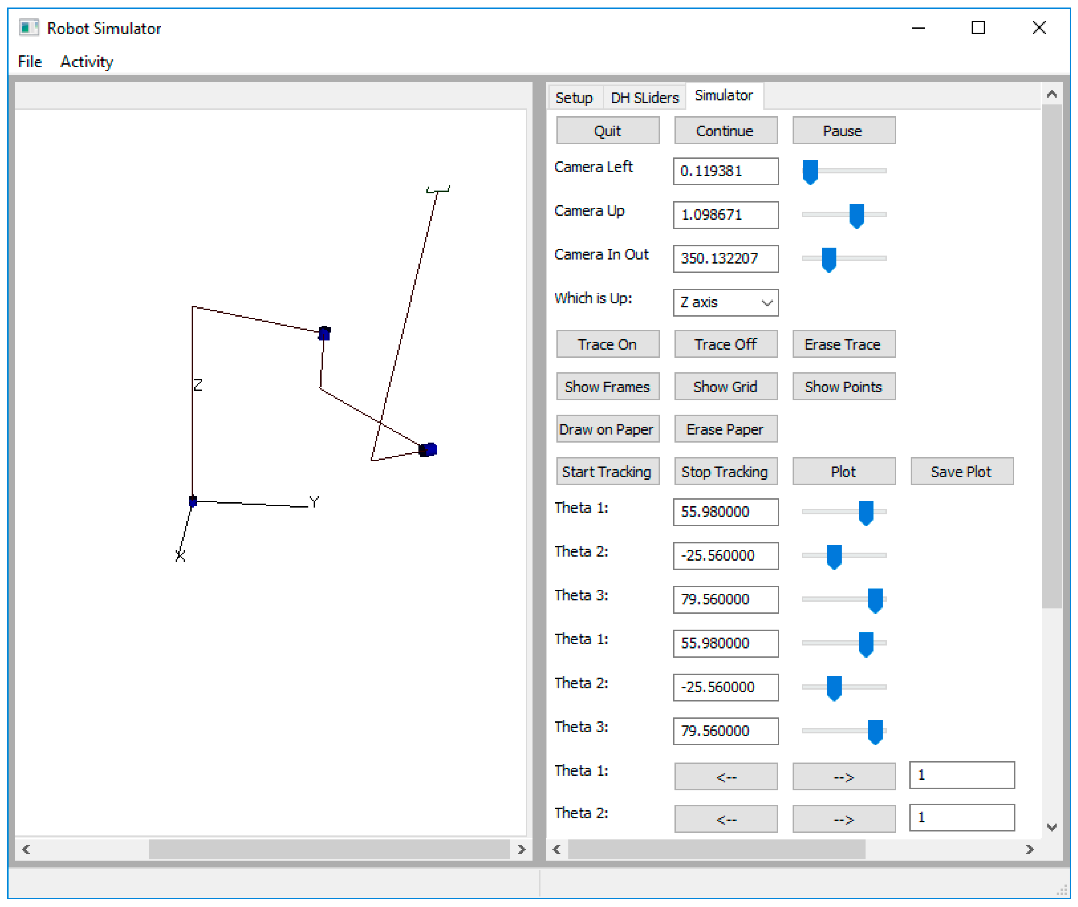
Figure 4.
Once the model is entered the user can move the joints individually and visually inspect the movement of the virtual arm to verify correctness of the model. The user can move the viewing angle as well.
Figure 4.
Once the model is entered the user can move the joints individually and visually inspect the movement of the virtual arm to verify correctness of the model. The user can move the viewing angle as well.

Figure 5.
The system components.

Figure 6.
The controlling side.
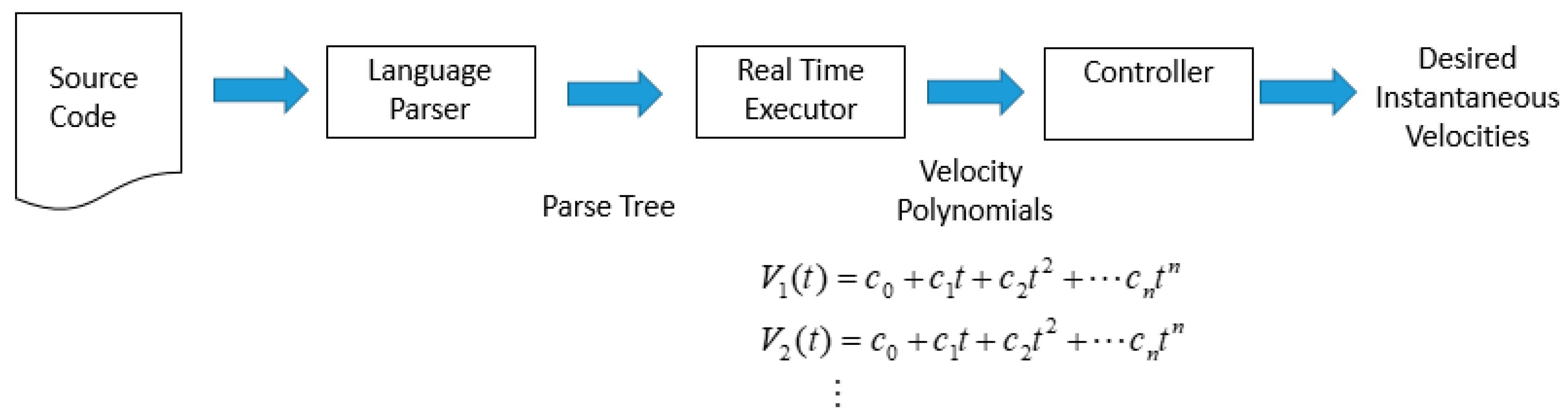
Figure 7.
The physical side.

Figure 8.
(a) The source code to solve and display a system of equations; (b) The program output.
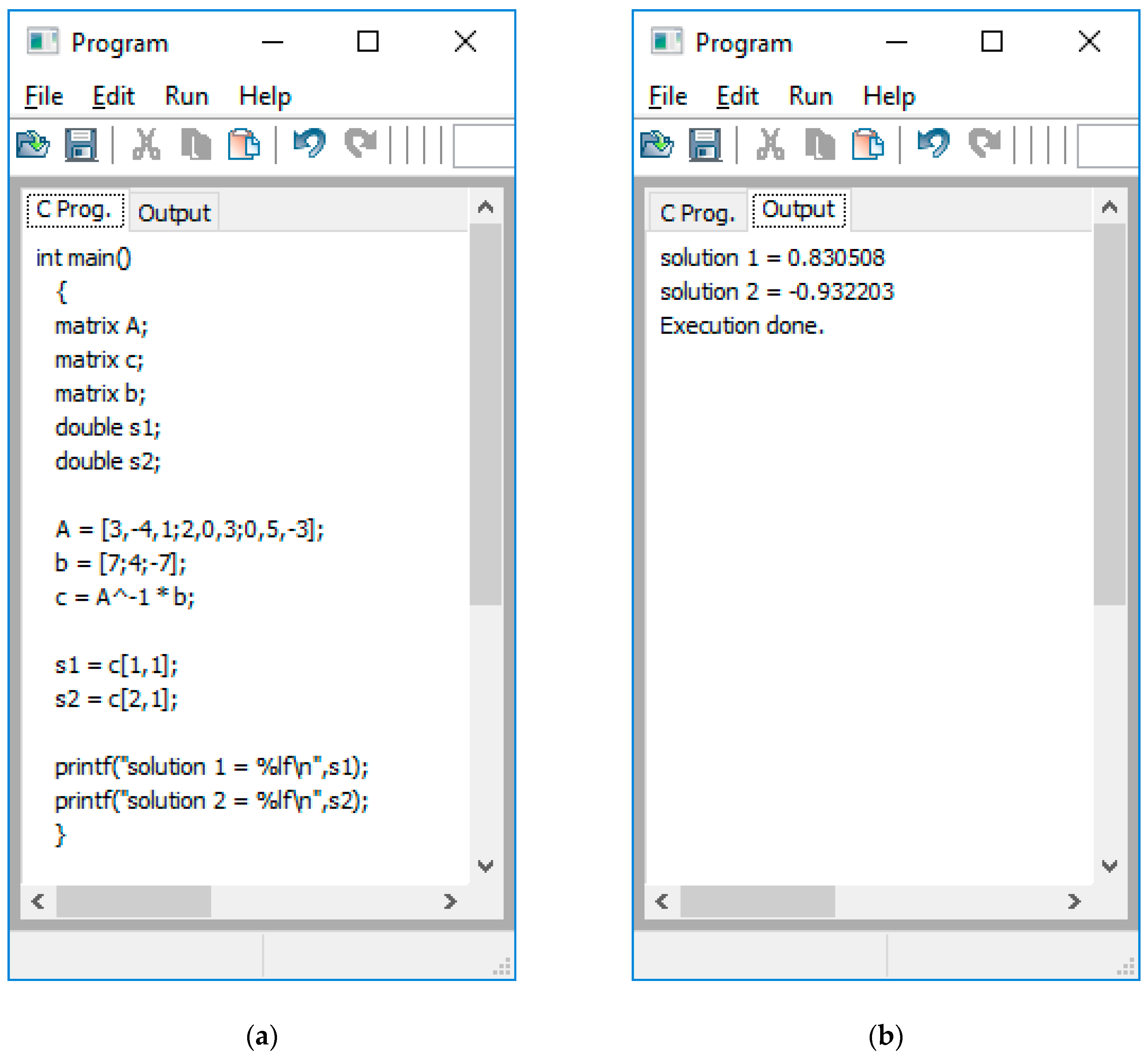
Figure 9.
(a) The factorial recursive function code; (b) The output.
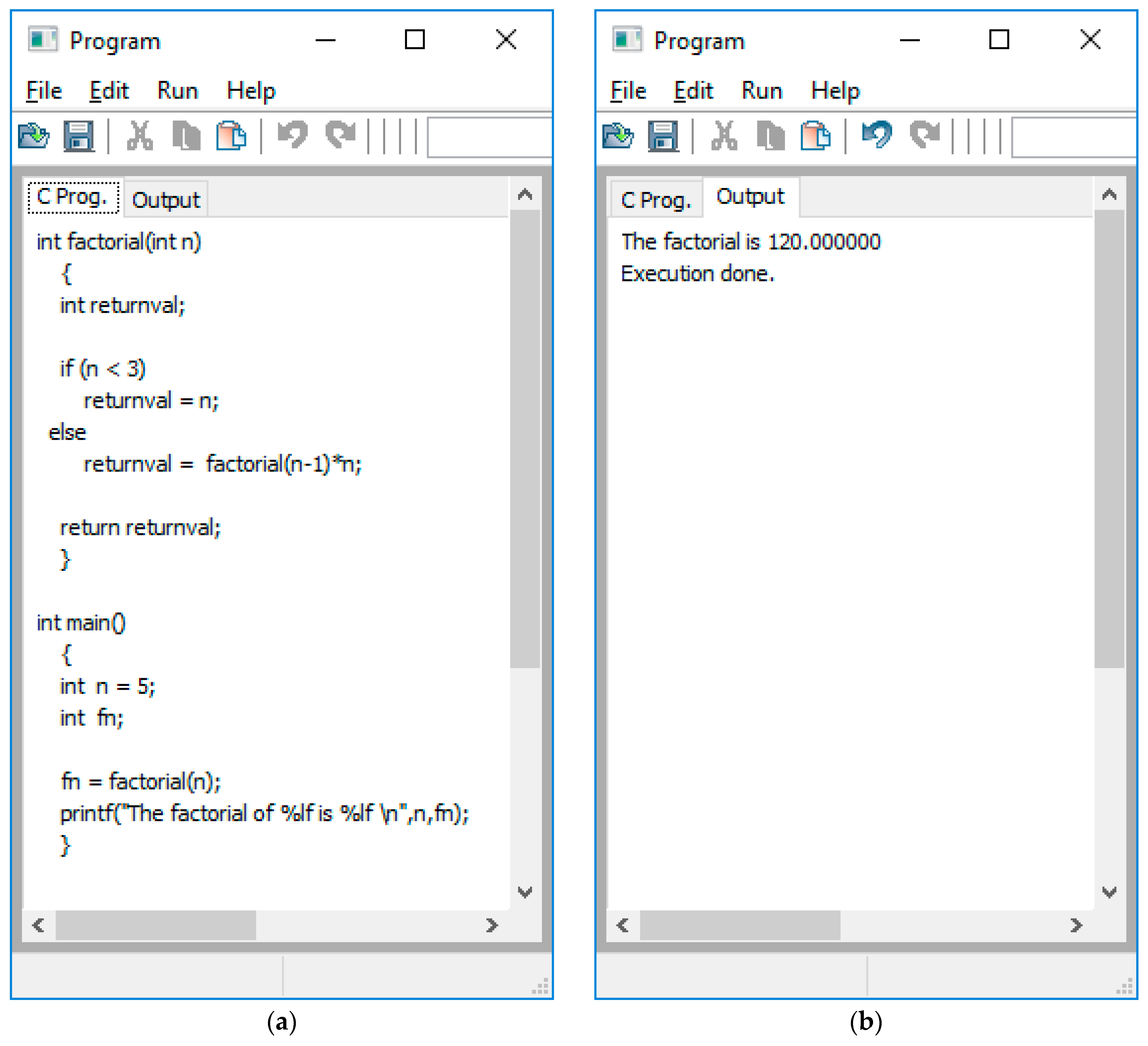
Figure 10.
Two link planar arm rendered by the tool shown in different positions.

Figure 11.
(a) The rendered arm’s start position; (b) Its end position.
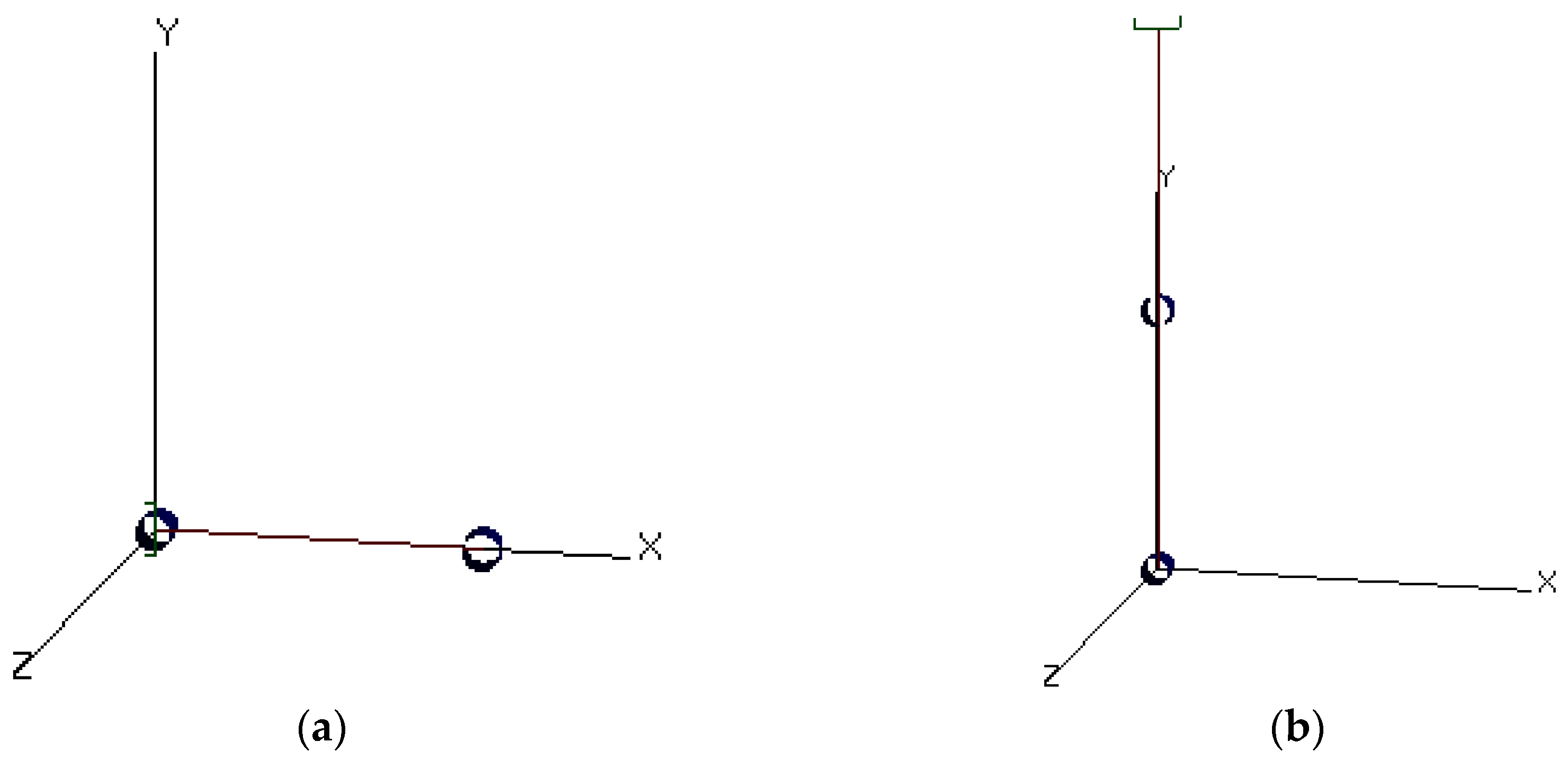
Figure 12.
The program for example assignment 1.
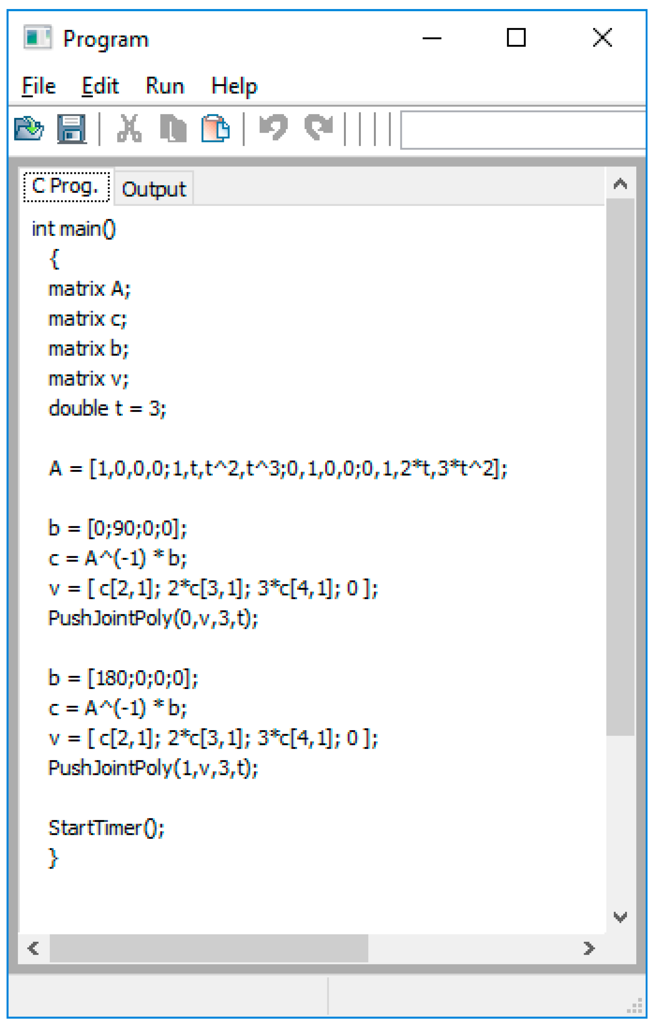
Figure 13.
The trace of the hand as the arm moves. The faster the hand moves, the greater the space between the dots.
Figure 13.
The trace of the hand as the arm moves. The faster the hand moves, the greater the space between the dots.
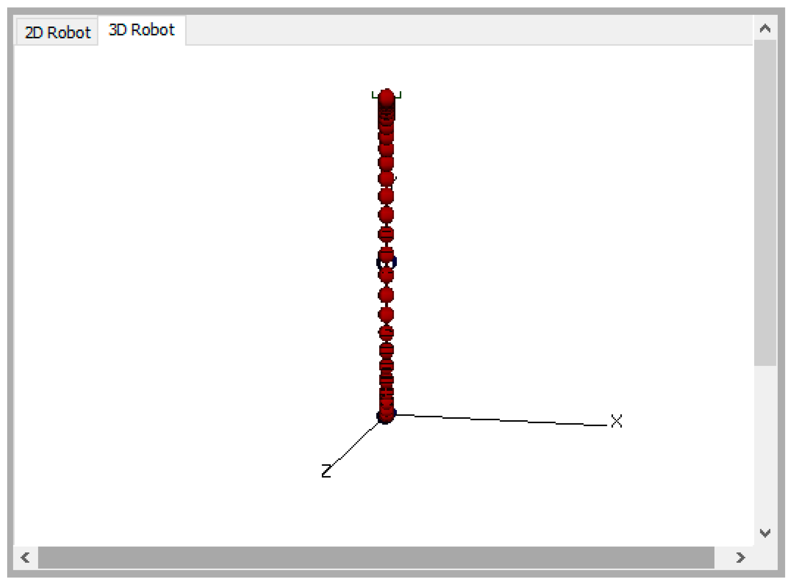
Figure 14.
(a) Plot of the position, velocity, and acceleration of trajectory for theta 1. The red is the position, blue the velocity and green the acceleration; (b) Plot of the position, velocity, and acceleration of trajectory for theta 2.
Figure 14.
(a) Plot of the position, velocity, and acceleration of trajectory for theta 1. The red is the position, blue the velocity and green the acceleration; (b) Plot of the position, velocity, and acceleration of trajectory for theta 2.
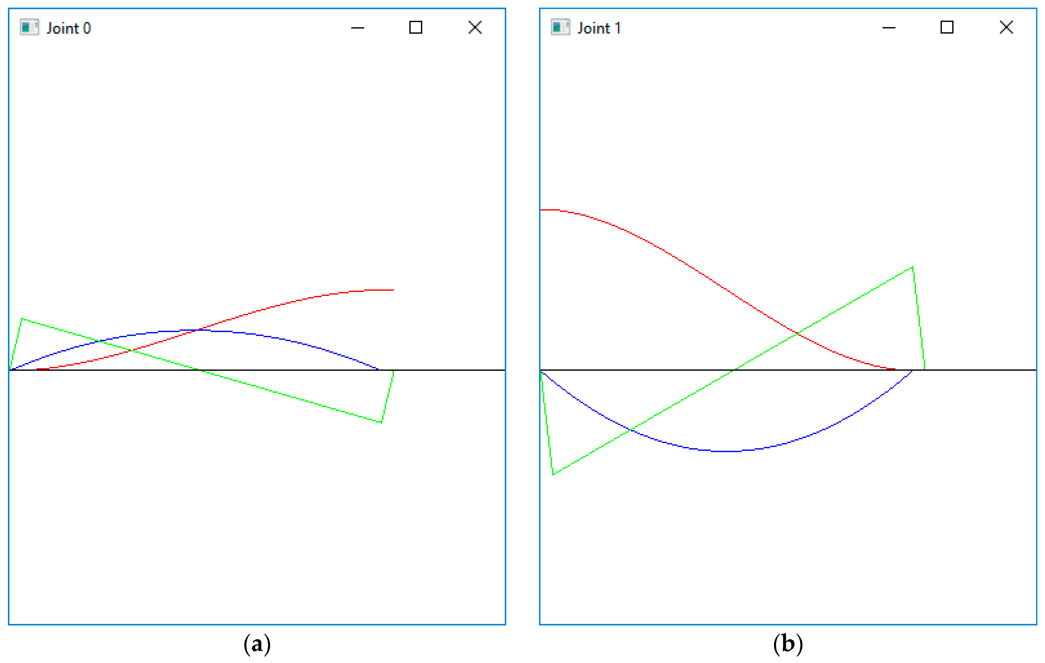
Figure 15.
The function to compute the velocity vector given the initial and final angle and the duration of movement.
Figure 15.
The function to compute the velocity vector given the initial and final angle and the duration of movement.
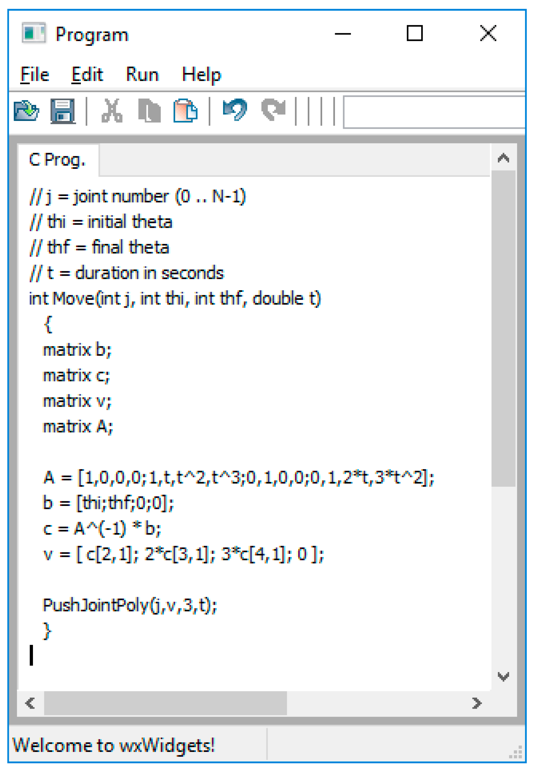
Figure 16.
The functions that compute the inverse kinematic equation for each joint.

Figure 17.
The function that moves the arm given the Cartesian coordinates to move to. It calls the other functions.
Figure 17.
The function that moves the arm given the Cartesian coordinates to move to. It calls the other functions.

Figure 18.
The main program for Assignment 2.

Figure 19.
The trace of the output path for Assignment 2.

Table 1.
The notation used in the equations.
| Symbol | Description |
|---|---|
| Acceleration | |
| MaxA | Maximum acceleration (from model) |
| Velocity | |
| Previous velocity | |
| Desired velocity | |
| Delta timeDelta time | |
| New position (joint angle) |
Table 2.
List of control structures, data types and legal operators.
| Control Structures | Variable Types | Standard Operators | Operator Description | Legal Operator for Matrices |
|---|---|---|---|---|
| if | int | &&, || | Logical | No |
| if-else | double | <, <=, >,>= | Compare | No |
| while | string | ==, != | Compare | No |
| for | matrix | +, − | Binary | Yes |
| *, / | Binary | Multiply only | ||
| ^ | Power | Yes | ||
| - | Unary | Yes | ||
| (,) | High Precedence | Yes |
Table 3.
The constraints derived.
| Joint 1 | Joint 2 |
|---|---|
| c | |
Table 4.
Response weights used to compute averages.
| Response | Weight |
|---|---|
| Strongly agree | 4 |
| Agree | 3 |
| Neutral | 2 |
| Disagree | 1 |
| Strongly disagree | 0 |
Table 5.
The survey questions along with their averaged response.
| Question | Average |
|---|---|
| 1. The tool helped me understand the Denavit and Hartenberg parameters used to model a robotic arm. | 3.0 |
| 2. The tool help me understand how a robotic arm moves given its virtual model. | 3.3 |
| 3. The tool helped me understand how to program the arm at the joint level by directly controlling each joint using polynomial trajectories. | 3.1 |
| 4. The tool helped me understand trajectory planning, the task of creating a trajectory for a joint. | 3.0 |
| 5. The tool help me understand inverse kinematics and its role in robot control. | 2.9 |
| 6. The tool help me understand how the material covered in this class is used to control a robot. | 3.3 |
| 7. The tool was helpful in allowing me to test the image processing and robotic vision methods covered in class. | 3.5 |
| 8. The tool help me understand the image processing and robotic vision material covered in class. | 3.3 |
| 9. The tool was easy to use. | 2.0 |
| 10. The tool was functional and any bugs found did not impede my ability to use the tool effectively. | 2.2 |
| 11. The compiler in the tool was easy to use. | 2.7 |
| 12. The C/MATLAB language used in the tool was easy to use and powerful and appropriate enough to perform the assignments. | 3.1 |
| 13. Overall, I am satisfied with the tool and recommend it be used in future classes. | 3.3 |
| 14. Overall, the tool was helpful in helping me learn the material covered in this course. | 3.4 |
© 2017 by the authors. Licensee MDPI, Basel, Switzerland. This article is an open access article distributed under the terms and conditions of the Creative Commons Attribution (CC BY) license (http://creativecommons.org/licenses/by/4.0/).
Share and Cite
MDPI and ACS Style
Gonzalez, F.; Zalewski, J. Teaching Joint-Level Robot Programming with a New Robotics Software Tool. Robotics 2017, 6, 41. https://doi.org/10.3390/robotics6040041
AMA Style
Gonzalez F, Zalewski J. Teaching Joint-Level Robot Programming with a New Robotics Software Tool. Robotics. 2017; 6(4):41. https://doi.org/10.3390/robotics6040041
Chicago/Turabian StyleGonzalez, Fernando, and Janusz Zalewski. 2017. "Teaching Joint-Level Robot Programming with a New Robotics Software Tool" Robotics 6, no. 4: 41. https://doi.org/10.3390/robotics6040041
Note that from the first issue of 2016, this journal uses article numbers instead of page numbers. See further details here.