Prediction Governors for Input-Affine Nonlinear Systems and Application to Automatic Driving Control


1
Department of Mechanical Engineering, Graduate School of Engineering, Osaka University, 2-1 Yamadaoka, Suita 565-0871, Japan
2
Graduate School of Information Science, Nara Institute of Science and Technology, 8916-5 Takayama-cho, Ikoma 630-0192, Japan
*
Author to whom correspondence should be addressed.
Robotics 2018, 7(2), 16; https://doi.org/10.3390/robotics7020016
Submission received: 26 February 2018
/
Revised: 29 March 2018
/
Accepted: 3 April 2018
/
Published: 4 April 2018
Abstract
:In recent years, automatic driving control has attracted attention. To achieve a satisfactory driving control performance, the prediction accuracy of the traveling route is important. If a highly accurate prediction method can be used, an accurate traveling route can be obtained. Despite the considerable efforts that have been invested in improving prediction methods, prediction errors do occur in general. Thus, a method to minimize the influence of prediction errors on automatic driving control systems is required. This need motivated us to focus on the design of a mechanism for shaping prediction signals, which is called a prediction governor. In this study, we first extended our previous study to the input-affine nonlinear system case. Then, we analytically derived a solution to an optimal design problem of prediction governors. Finally, we applied the solution to an automatic driving control system, and demonstrated its usefulness through a numerical example and an experiment using a radio controlled car.
1. Introduction
In recent years, automatic driving control has attracted attention, and various studies on this topic have been undertaken [1,2]. In automatic driving systems that achieve lane-keeping and obstacle avoidance, the traveling route is predicted based on the data of the driving environment collected using sensor information from cameras and other equipment mounted on the vehicle [3,4]. Acceleration and braking are then controlled to move the vehicle along the predicted traveling route. Accordingly, the predicting of the traveling route is crucial for achieving sophisticated automatic driving control. Although it may be possible to obtain an accurate traveling route if it can be predicted using a vast amount of data and a sophisticated prediction algorithm, it is very likely that, if the amount of data available is small and the prediction algorithm is simple, the accuracy of the predicted traveling route will be inferior.
Based on this perspective, many previous studies have been conducted on image recognition as a means of recognizing the driving environment with high prediction accuracy [5,6,7]. Moreover, many studies have been conducted on various prediction methods, such as Kalman filtering and machine learning, and automatic driving control systems based on such methods have been proposed [8,9,10,11,12,13]. However, the prediction method, regardless of its accuracy, may produce prediction errors that are unavoidable in an unpredictable real-world situation. Accordingly, methods to minimize the degradation incurred in the performance of automatic driving control when a prediction error occurs are deemed necessary.
In the field of control, an optimal prediction governor, whereby the predicted signal is shaped to minimize the decrease in the control performance of the system when a prediction error occurs, has been proposed [14]. In an optimal prediction governor, the low accuracy predicted value obtained in real time, is proactively shaped using a past high accuracy predicted value and the system model information. In an autonomous driving system, in addition to the predicted value obtained in real time, in many cases it is also possible to use highly accurate predicted information obtained from time-consuming processing, such as image recognition, and therefore, the applicability of the prediction governor to automatic driving problems is considered to be high. However, only linear systems are considered in the optimal prediction governor, making it inapplicable directly to nonlinear systems such as automotive systems.
Motivated by the above, this paper is focused on the design of an optimal prediction governor for nonlinear systems. First, a generalized version of the prediction governor designed in our previous study is considered. Then, the optimal design problem for the prediction governor is formulated for application to input-affine nonlinear systems. The optimality here refers to the shaping of the low accuracy predicted value by the prediction governor, such that the system output obtained using this shaped value becomes the best approximation of the system output obtained using the high accuracy predicted value as input. Next, the optimal design problem is analytically solved to derive the optimal prediction governor and clarify the optimal structure. Finally, the application of the proposed prediction governor to an automatic driving control problem is described. In particular, the usefulness of the prediction governor is validated through the result of a trajectory tracking simulation and an experiment on lane-keeping control using a radio controlled car.
The following points are emphasized. First, in this study, the prediction governor proposed in our previous study [14] was generalized, and an optimal prediction governor for input-affine nonlinear systems was derived. Consequently, the prediction governor was rendered applicable to not only linear, but also nonlinear systems. This is a significant and successful outcome in terms of developing optimal design theory for prediction governors. Next, the prediction governor was applied to an automatic driving control system, and the usefulness of the proposed method was validated through numerical simulations and experiments. Based on this initiative, it is likely that the practical applicability of the prediction governor can be demonstrated. Moreover, to be best of the authors’ knowledge an approach that considers the reshaping of predicted signals in automatic driving control has not previously been reported. Accordingly, the successful outcome of the present study gives new insight into automatic driving technology.
Finally, we make the following remark. The approach of this paper is similar to a path smoothing approach based on model information of systems for non-holonomic vehicles [15]. However, the proposed perdition governor shapes predicted signal with prediction error in order to minimize the performance degradation due to prediction error. This point is different from the previous work in [15]. In addition, the prediction governor is similar to reference governor [16,17]. However, the prediction governor is distinguished from the reference governor in terms of concept and structure. The main purpose of the prediction governor is to minimize the influence of the prediction error on the system’s output, while that of the reference governor is to eliminate wind up phenomenon due to the input/state constraints of systems. Moreover, the basic reference governor is given by , where is a given original reference signal, v is a modified reference signal, and the parameter is maximized by considering input/state constraints. Thus, the reference governor is based on the original desired reference signal and the model information, and minimizes the value of under input/state constraints. In contrast, the prediction governor is based on the predicted low accuracy signal , the past high accuracy signal , and the model information. In addition, it minimizes the output difference between the system driven by the shaped signal v and that driven by .
This paper presents an extension of the authors’ previous study [18], with the addition of a proof of the optimality for the derived prediction governor and the results of an experiment using a radio controlled car.
Notations: Let , , and be the real number field, the set of positive real numbers, and the set of positive integers, respectively. We use to express the identity matrix. The ∞-norm of discrete-time signal is expressed by .
2. Optimal Prediction Governor for Input-Affine Nonlinear Systems
2.1. Problem Formulation
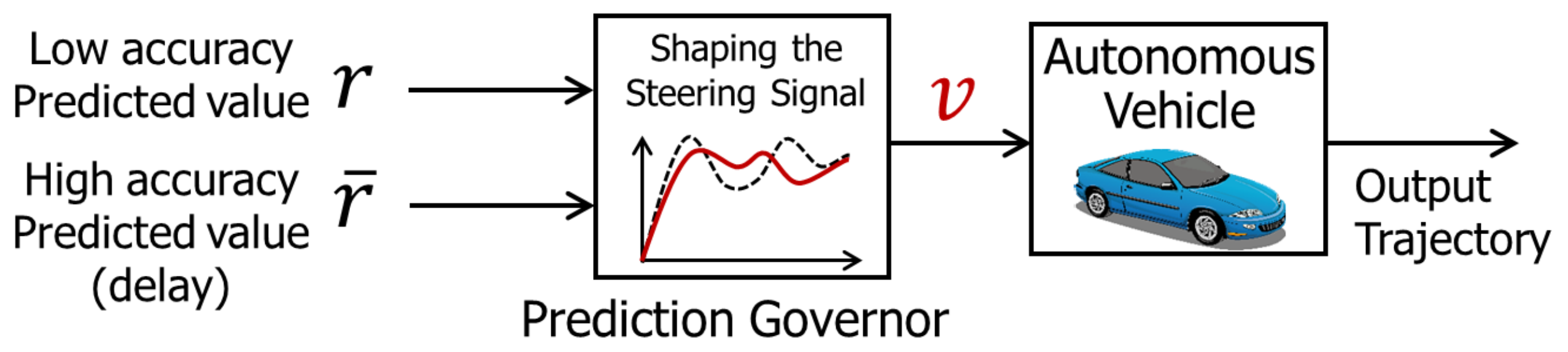
Consider the feedforward system shown in Figure 1, which is composed of the control system and the prediction governor G.
The input-affine nonlinear system is given by
where is discrete time, is the state, is the input, and is the output. For , the initial state of x is given by . In addition, and are continuous and smooth functions of x and is constant matrix. We assume the state x of system is bounded, i.e., holds for every initial state and bounded input . Furthermore, we assume that .
The prediction governor is given by
where is the state, and are the inputs, is the output, and . and are the functions of . For G, we assume that to guarantee for and . The prediction governor in (2) is a general version of that presented in the previous study [14]. In Figure 1, r is a low accuracy predicted reference and a high accuracy predicted reference. In addition, u is a past high accuracy predicted reference, and in this study it is assumed that and . In this study, we also assume that the maximum error between low accuracy predicted reference r and high accuracy predicted reference is .
The state and the output of system driven by the high accuracy predicted signal are denoted by and , respectively. In addition, . Then, we derive a prediction governor that minimizes the difference between the output y of and the output in Figure 1. To design the prediction governor, we introduce the following cost function:
Function evaluates the maximum difference between y and . Then, the design problem of prediction governor G is formulated as follows.
Problem 1.
Suppose that the control system Σ and are given. Then, find the parameters , , , , , , α, β, γ of prediction governor G that minimize the value of in (4). In addition, determine the minimum value of .
By using a solution to the problem, the output behavior of system is similar to that of system G with high accuracy predicted reference .
2.2. Optimal Prediction Governor
By using and the new variable ( from (3)), the above equation can be rewritten as
Then, we obtain
from (6), , and . This means that the lower bound of is given by for and . Therefore, if there exists a prediction governor G such that the relations , and hold, such a G is an optimal solution to Problem 1.
The solution to Problem 1 is given as follows.
Theorem 1.
For the nonlinear system Σ, an optimal prediction governor is given by
and . In addition, the minimum value of is given by
Proof of Theorem 1.
By direct calculation, it is determined that the relations and hold for (8) and .
Next, for the minimum value of , the following relations hold.
Note that is the output of system with . First, (10) is obtained from (7). Then, (11) and (12) are obvious from their definitions. Finally, the proof of (13) is given as follows.
The output of system with in (8) is expressed as
Here, the state corresponds to the state x of system driven by v, i.e., , and the state corresponds to of driven by , i.e., , because has the model of . Based on this, (14) can be rewritten:
Therefore, the output difference between and at is
For any and , we have
From this,
can be obtained, which means (13) holds. ☐
Theorem 1 assigns the prediction governor G that minimizes and the performance limit of the prediction governor given by (2). The following procedure is followed for implementing (8).
- (i)
- Calculate in the first formula.
- (ii)
- Using the second formula, calculate .
- (iii)
- Using the third formula, calculate .
- (iv)
- Calculate in the first formula.
Next, the structure of the prediction governor obtained from Theorem 1 is explained. First, and in (8) correspond to the system state x at the time of the input of shaped value v and the system state at the time of the input of high accuracy predicted value , respectively. That is, the first and second formulas in (8) estimate and . Next, in the output formula for in (8), is shaped based on the estimation of the difference in outcome, i.e., difference between and , due to prediction error. In other words, the optimal prediction governor can be considered to produce a compensating signal to cancel the output difference generated one step ahead as a result of prediction error.
Moreover, the boundedness of the state of the optimal prediction governor can be confirmed as follows. From the third row of the first formula in (8), the state is bounded if the state of the nonlinear system is bounded for . At this time, from the second row of the first formula in (8), it can be confirmed that the state is bounded. In addition, substituting v from the third formula in the first row of the first formula in (8) gives
where . This means the state is bounded if the state of the system given by (19) is bounded for . Therefore, if the states of system and the system given by (19) are bounded for , , then the state of the optimal prediction governor is bounded, i.e., .
Finally, some supplementary points are now discussed. When system is linear, that is, in case
Theorem 1 agrees with the results obtained in the previous study [14]. In fact, by substituting , in (8), together with coordinate transformation and dimensionality reduction from to n, give
where , , and . Based on these findings, it can be confirmed that, for a linear system, the performance of the prediction governor cannot be improved even if the prediction governor class is extended as given by (2).
3. Application to Automatic Driving Control
In this section, the application of the prediction governor to an automatic driving control system is described, and its usefulness is examined. A steering signal, as shown in Figure 2, is shaped by combining low accuracy prediction, where real-time processing is feasible, and high accuracy prediction, where the processing is time consuming. The car is controlled using this shaped steering signal.
First, to verify the prediction governor’s performance, a numerical simulation of trajectory tracking was conducted and the tracking accuracy was evaluated. Next, to examine the usefulness of the prediction governor, actual lane-keeping experiments were conducted using a radio controlled car.
3.1. Simulation
Let us consider system in Figure 1. System is a four-wheel car model and is given by
where is the sampling time and V is the vehicle translation speed (constant). x denotes the state of and is defined by (initial value ) in terms of the vehicle position () and the yaw angle . v is the input corresponding to the the vehicle yaw rate. y is the output response, where is set by focusing on vehicle yaw angle . Moreover, in , the predicted values r and are the target yaw rates for the four-wheel car, where r is the low accuracy predicted value and is the high accuracy predicted value.
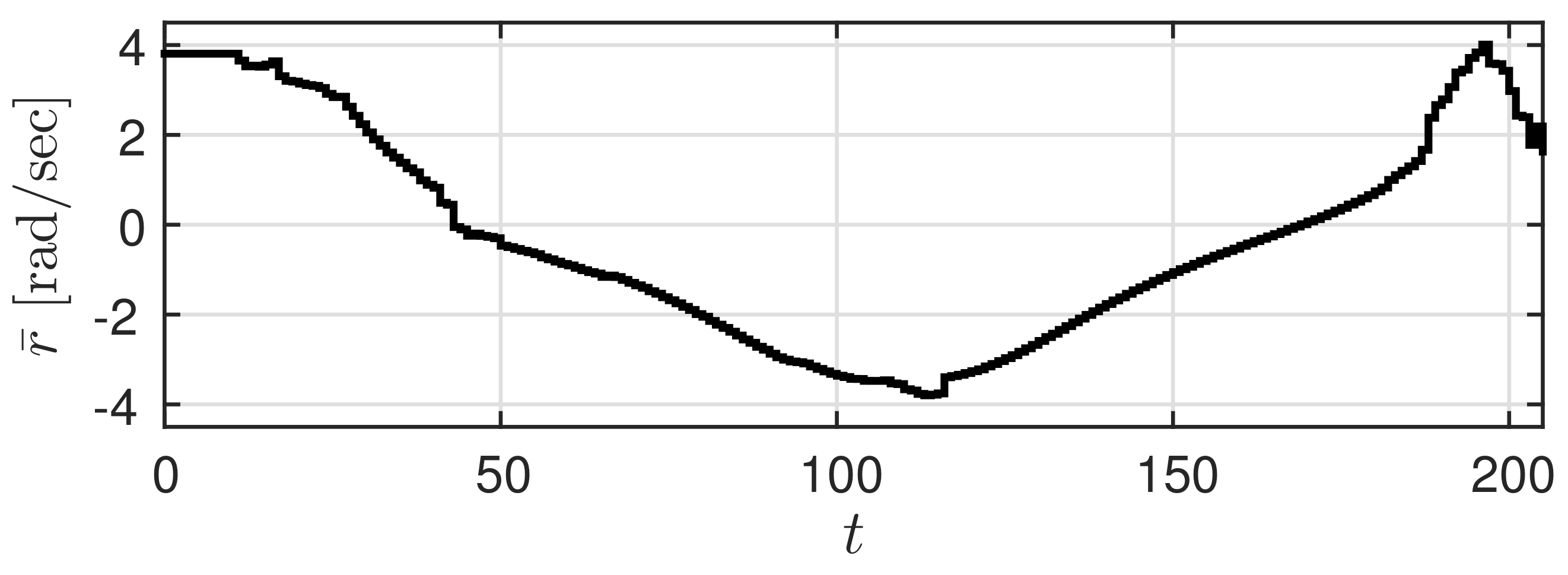
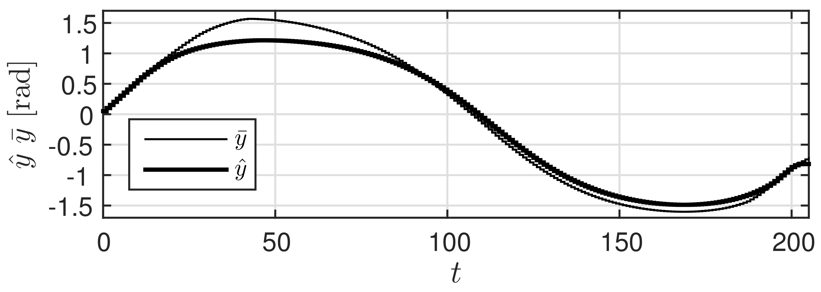
Let us suppose (s) and (mm/s). Let the low accuracy predicted value be given by Figure 3, and the high accuracy predicted value obtained with a slight delay be given by Figure 4 ( is the maximum value of ). Here, a trajectory that needs to be realized by the car (true trajectory) is set for the high accuracy predicted value and a trajectory that deviates slightly from this trajectory is set for the low accuracy predicted value. At this time, r is shaped using prediction governor G, generating the shaped value v. The results of using the prediction governor are shown in Figure 5. Figure 5a shows the shaped value v and Figure 5b shows the output response y of .
In Figure 5b, the thin line represents the system response (behavior of yaw angle ) using the high accuracy predicted value from Figure 4, while the thick line represents the system response y (behavior of yaw angle ) using the shaped value v. It can be observed that the two responses overlap. In contrast, Figure 6 shows the result (behavior of yaw angle ) obtained using the low accuracy predicted value r. Further, Figure 7 shows the trajectory of the car along the plane. In this figure, the dashed line, the dot-dashed line, and the solid line represent the trajectories obtained using , r, and v, respectively. These figures confirm that the response obtained using shaped value v is closer to the output response obtained using than that obtained using r. At this time, the value of was 0.0282 and that of was 0.3693. These results confirm that the prediction governor was operating appropriately. Moreover, the calculated value of the right hand side of (9) was 0.0282. This suggests that it is possible to estimate in advance the difference in outcome.
3.2. Experiment
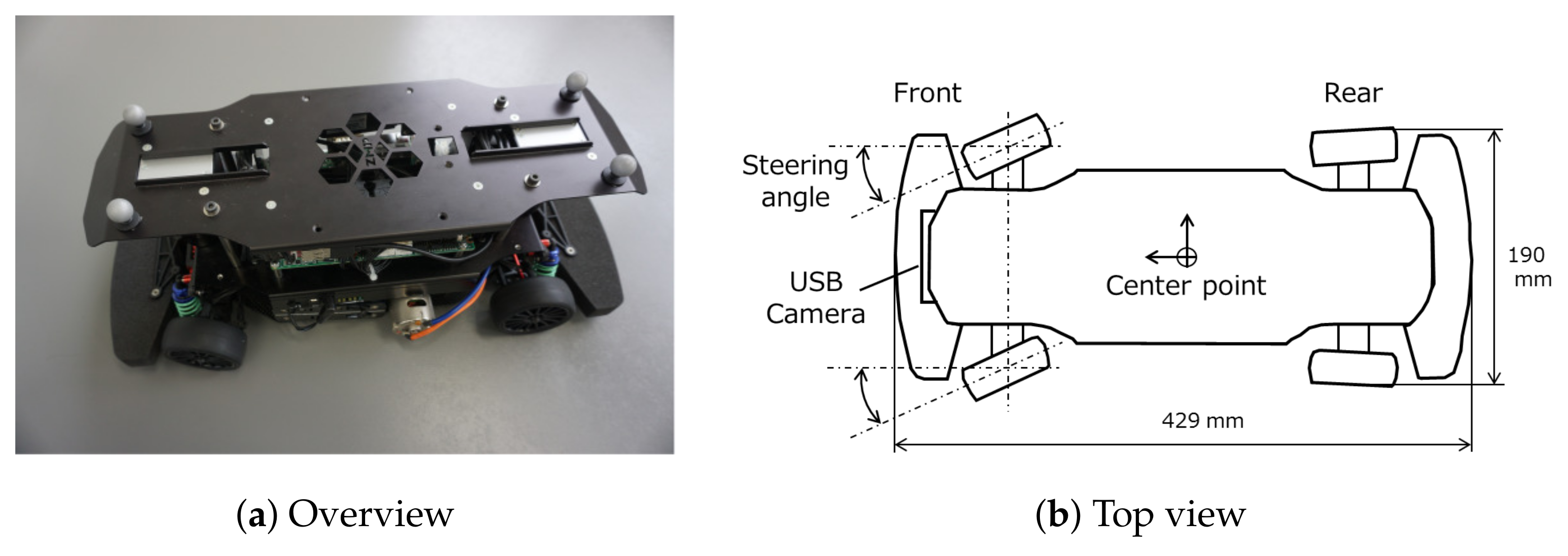
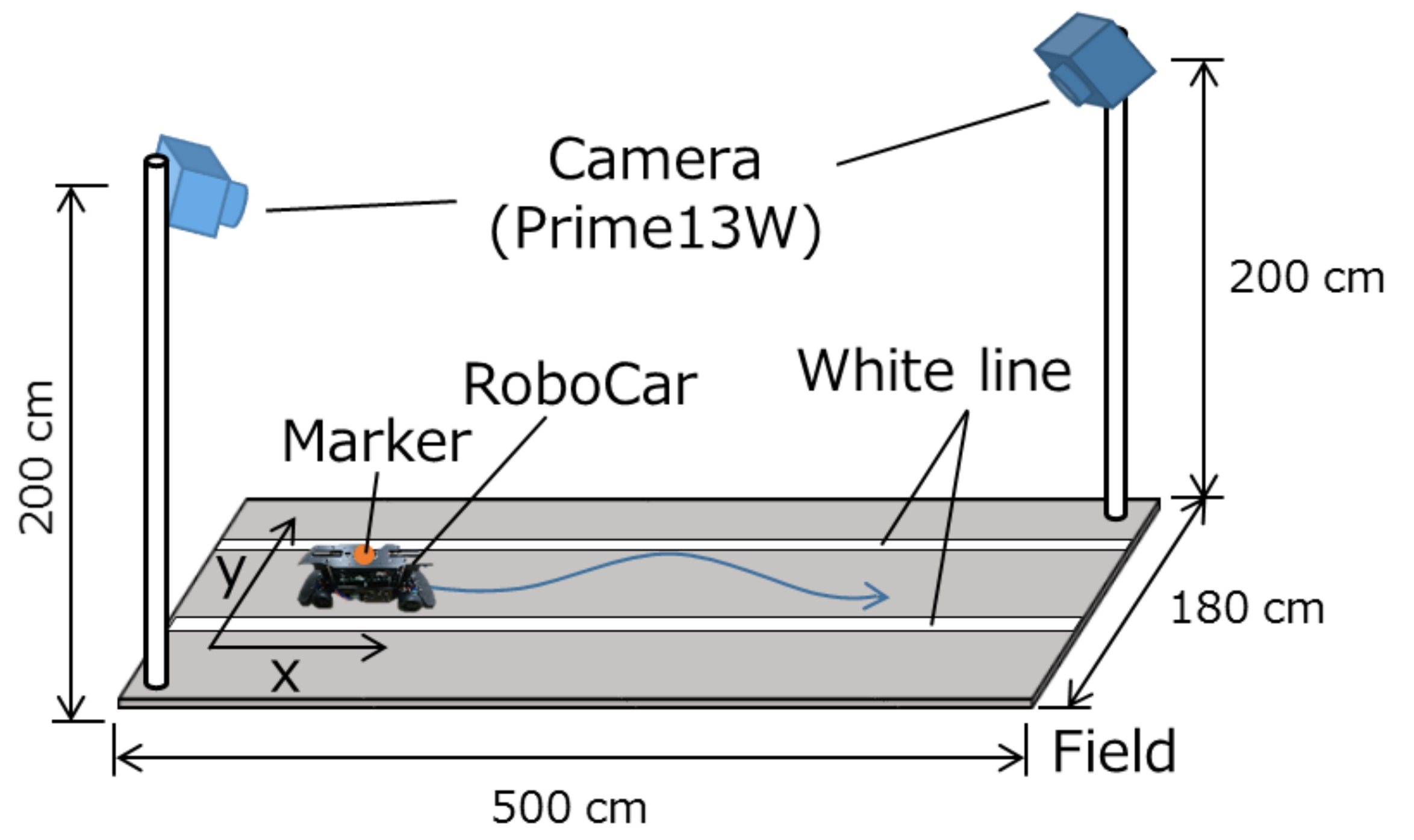
A RoboCar 1/10 2016 from ZMP Inc., as shown in Figure 8, was used in the experiments. Table 1 shows the specification of the RoboCar. Figure 9 shows the experimental setup. Two white lines were drawn on the field. As depicted in Figure 9, position measurement cameras (OptiTrack Prime13W) were placed at both ends of the field to capture the RoboCar’s travel trajectory. First, the image captured by the camera mounted on the RoboCar was obtained and the traveling route was predicted by analyzing this image. Next, based on the predicted route the steering angle of the RoboCar was controlled.
In the process of predicting the traveling route, two types of image processing algorithms were used. In the first algorithm (Image Processing 1), the images captured by the camera were converted to binary images, and from the images corresponding to the position of the white lines 300 (mm) ahead of the front end of the car the coordinates on the image were determined. The mid point between the white lines was then calculated using these coordinates. In the second algorithm (Image Processing 2), after binarization, using a differential filter and Hough transformation together with processing such as clustering, the white lines were detected. The crossing point (vanishing point) of these two lines was then calculated. In this study, the aforementioned two methods of image processing were executed simultaneously in the RoboCar.
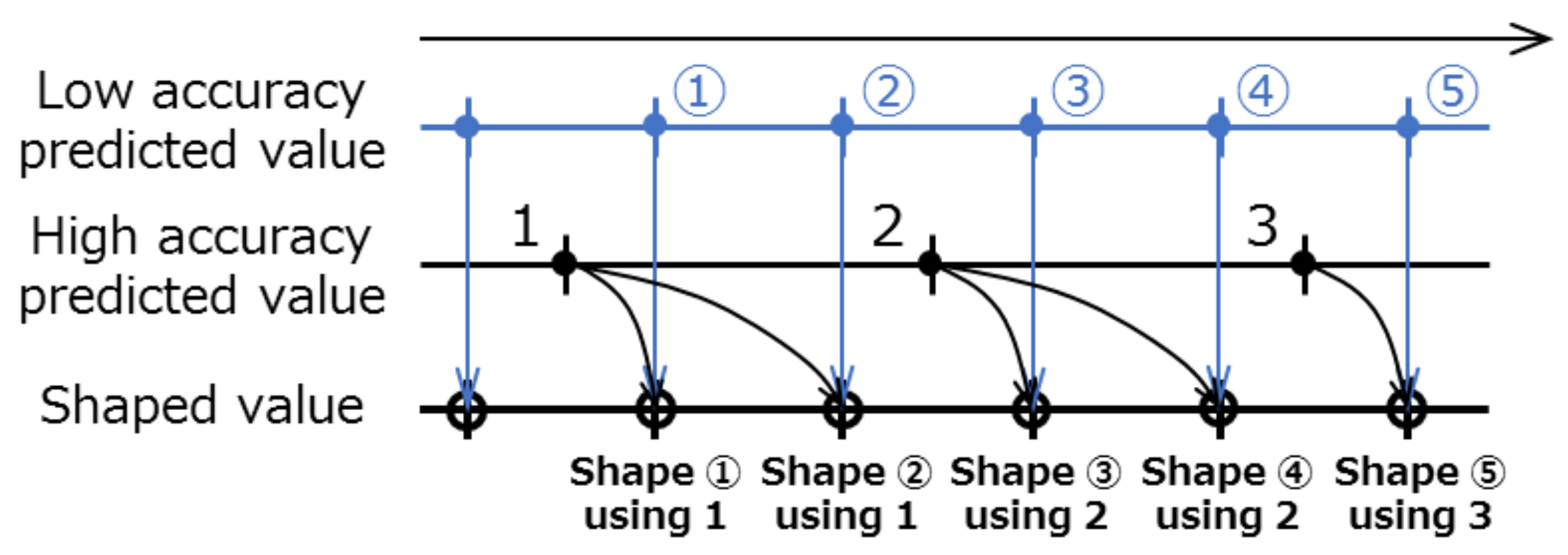
As shown in Figure 10, for a sampling period of = 0.07 (s), although Image Processing 1 can be conducted in real time, there is a time lag for Image Processing 2, as it requires more time. In this study, based on experiments conducted in advance to estimate the white line position, the yaw rate signal obtained using the results of Image Processing 1 was set as the low accuracy predicted value, and the yaw rate signal obtained using the results of Image Processing 2 was set as the high accuracy predicted value. Using the prediction governor, in each step, the low accuracy predicted value was then shaped using the high accuracy predicted value, and the RoboCar was run using this shaped value.
Since the actual input to the RoboCar is the steering angle, the yaw rate signal v is used after converting it into steering angle s (rad) using the transformation . Here, L is the distance between the front and rear wheel axles and was set as (mm) in the experiments V is the speed of the car and was set at a constant value of (mm/s).
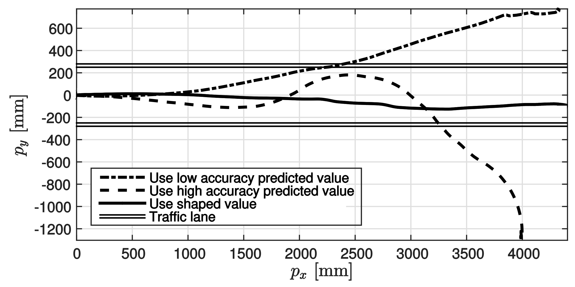
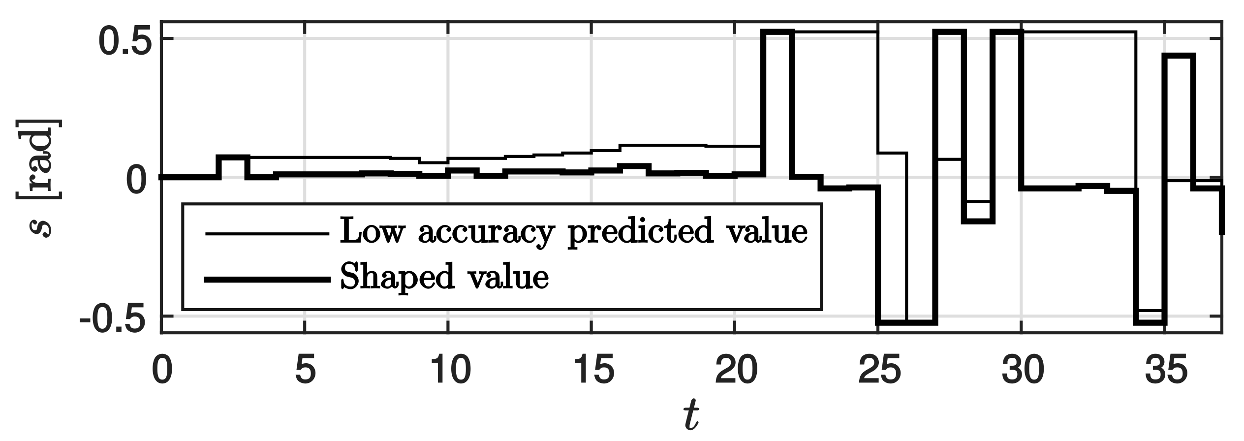
The results of the experiments are shown in the following figures. The results of applying the prediction governor, as shown in Figure 11, suggest that the steering angle represented by the thin line is shaped as indicated by the thick line. The corresponding trajectories are shown in Figure 12. In Figure 12, the double lines show the two white lines of the traffic lane. The dot-dashed line shows the trajectory when the low accuracy predicted value only was used, the dashed line shows the trajectory when the high accuracy predicted value only was used, and the solid line shows the trajectory when the nonlinear prediction governor was used in driving control. As observed in the results, first, the travel trajectory based on low accuracy predicted value only deviated widely from the traffic lane because of misrecognition of the white lines. Further, the travel trajectory based on the high accuracy predicted value only, deviated from the traffic lane because of the time lag. In contrast, by applying the prediction governor, the erroneous steering signal was shaped and deviation from the traffic lane was avoided. The results confirmed that the control performance was improved by applying the prediction governor. Finally, it is also stressed that a satisfactory performance could be obtained by using the prediction governor even though a controller was designed without the consideration of lane-keeping constraints. Therefore, this experimental result illustrated the practical benefits of the proposed method.
4. Conclusions
In this paper, a prediction governor for input-affine nonlinear systems was proposed. First, the optimal design problem for the prediction governor was formalized, and the optimal prediction governor was analytically derived. Next, the simulation of trajectory tracking and lane-keeping experiments using actual model car to confirm the feasibility of applying the proposed approach in automatic driving control problem were described. Finally, it was confirmed that desirable behavior can be obtained in automatic driving control by applying the prediction governor.
As topics of study in the future, the design of a prediction governor for MIMO systems and systems where , as well as experiments using actual cars taking into account even more complex environments such as driving along curved traffic lanes etc., are suggested.
Acknowledgments
The author would like to thank Professor Kenji Sugimoto, Nara Institute of Science and Technology for his support. This research was partly supported by JSPS KAKENHI (16H06094).
Author Contributions
Y.M. and Y.I. developed the optimal prediction governor, Y.I. performed the experiments and analyzed the data, and Y.M. and Y.I. wrote the paper.
Conflicts of Interest
The authors declare no conflict of interest.
References
- Maurer, M.; Gerdes, J.; Lenz, B.; Winner, H. Autonomous Driving: Technical, Legal and Social Aspects; Springer Publishing Company: New York, NY, USA, 2016. [Google Scholar]
- Bimbraw, K. Autonomous cars: Past, present and future a review of the developments in the last century, the present scenario and the expected future of autonomous vehicle technology. In Proceedings of the 2015 12th International Conference on Informatics in Control, Automation and Robotics (ICINCO), Alsace, France, 21–23 July 2015; pp. 191–198. [Google Scholar]
- Shackleton, C.J.; Kala, R.; Warwick, K. Sensor-Based Trajectory Generation for Advanced Driver Assistance System. Robotics 2013, 2, 19–35. [Google Scholar] [CrossRef]
- Thanpattranon, P.; Ahamed, T.; Takigawa, T. Navigation of an Autonomous Tractor for a Row-Type Tree Plantation Using a Laser Range Finder—Development of a Point-to-Go Algorithm. Robotics 2015, 4, 341–364. [Google Scholar] [CrossRef]
- Timofte, R.; Zimmermann, K.; Van Gool, L. Multi-view traffic sign detection, recognition, and 3D localisation. Mach. Vis. Appl. 2014, 25, 633–647. [Google Scholar] [CrossRef]
- Mogelmose, A.; Trivedi, M.M.; Moeslund, T.B. Vision-Based Traffic Sign Detection and Analysis for Intelligent Driver Assistance Systems: Perspectives and Survey. IEEE Trans. Intell. Transp. Syst. 2012, 13, 1484–1497. [Google Scholar] [CrossRef]
- Ozgunalp, U.; Fan, R.; Ai, X.; Dahnoun, N. Multiple Lane Detection Algorithm Based on Novel Dense Vanishing Point Estimation. IEEE Trans. Intell. Transp. Syst. 2017, 18, 621–632. [Google Scholar] [CrossRef]
- Hara, K.; Saito, H. Vehicle Localization Based on the Detection of Line Segments from Multi-Camera Images. J. Rob. Mechatron. 2015, 27, 617–626. [Google Scholar] [CrossRef]
- Kazama, K.; Akagi, Y.; Raksincharoensak, P.; Mouri, H. Fundamental Study on Road Detection Method Using Multi-Layered Distance Data with HOG and SVM. J. Rob. Mechatron. 2016, 28, 870–877. [Google Scholar] [CrossRef]
- Mammeri, A.; Boukerche, A.; Tang, Z. A real-time lane marking localization, tracking and communication system. Comput. Commun. 2016, 73 Pt A, 132–143. [Google Scholar] [CrossRef]
- Li, Q.; Chen, L.; Li, M.; Shaw, S.L.; Nuchter, A. A Sensor-Fusion Drivable-Region and Lane-Detection System for Autonomous Vehicle Navigation in Challenging Road Scenarios. IEEE Trans. Veh. Technol. 2014, 63, 540–555. [Google Scholar] [CrossRef]
- Gerla, M.; Lee, E.K.; Pau, G.; Lee, U. Internet of vehicles: From intelligent grid to autonomous cars and vehicular clouds. In Proceedings of the 2014 IEEE World Forum on Internet of Things (WF-IoT), Seoul, Korea, 6–8 March 2014; pp. 241–246. [Google Scholar]
- Hashimoto, M.; Matsui, Y.; Takahashi, K. Moving-Object Tracking with In-Vehicle Multi-Laser Range Sensors. J. Rob. Mechatron. 2008, 20, 367–377. [Google Scholar] [CrossRef]
- Minami, Y.; Azuma, S. Prediction governors: Optimal solutions and application to electric power balancing control. In Proceedings of the 54th IEEE Conference on Decision and Control, Osaka, Japan, 15–18 December 2015; pp. 1126–1129. [Google Scholar]
- Andreasson, H.; Saarinen, J.; Cirillo, M.; Stoyanov, T.; Lilienthal, A.J. Drive the Drive: From Discrete Motion Plans to Smooth Drivable Trajectories. Robotics 2014, 4, 400–416. [Google Scholar] [CrossRef]
- Garone, E.; Di Cairano, S.; Kolmanovsky, I.V. Reference and command governors for systems with constraints: A survey on theory and applications. Automatica 2017, 75, 306–328. [Google Scholar] [CrossRef]
- Di Cairano, S.; Kalabić, U.V.; Kolmanovsky, I.V. Reference governor for network control systems subject to variable time-delay. Automatica 2015, 62, 77–86. [Google Scholar] [CrossRef]
- Iwai, Y.; Minami, Y.; Sugimoto, K. Prediction Governor for Nonlinear Affine Systems and Its Application to Automatic Cruise Control. In Proceedings of the SICE Annual Conference 2017, Kanazawa, Japan, 19–22 September 2017; pp. 1336–1339. [Google Scholar]
Figure 1.
Error system composed of a control system and a prediction governor.
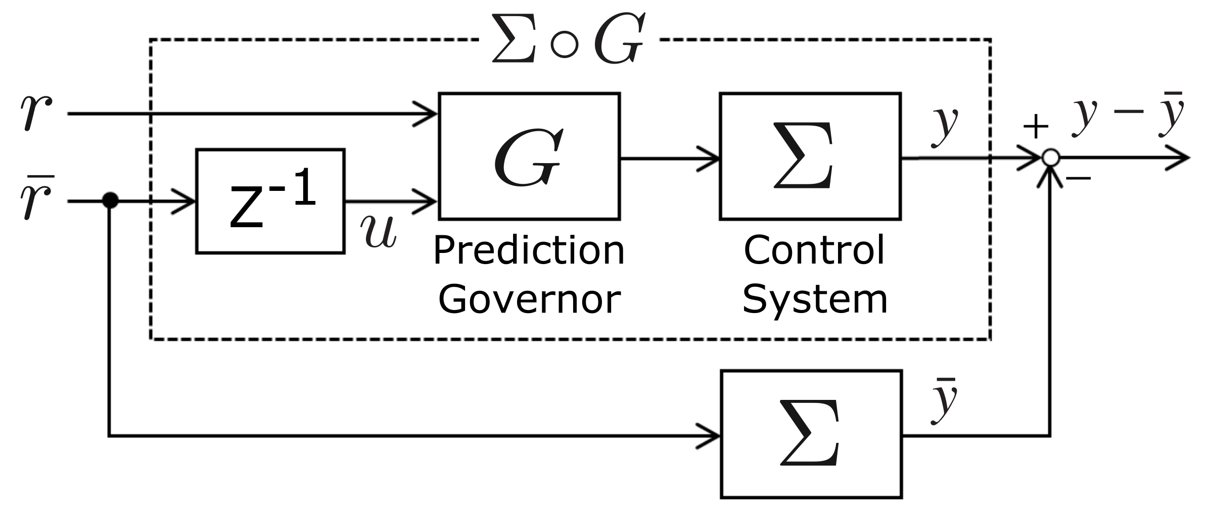
Figure 2.
Application of the prediction governor to autonomous vehicle.

Figure 3.
Low accuracy predicted value r.
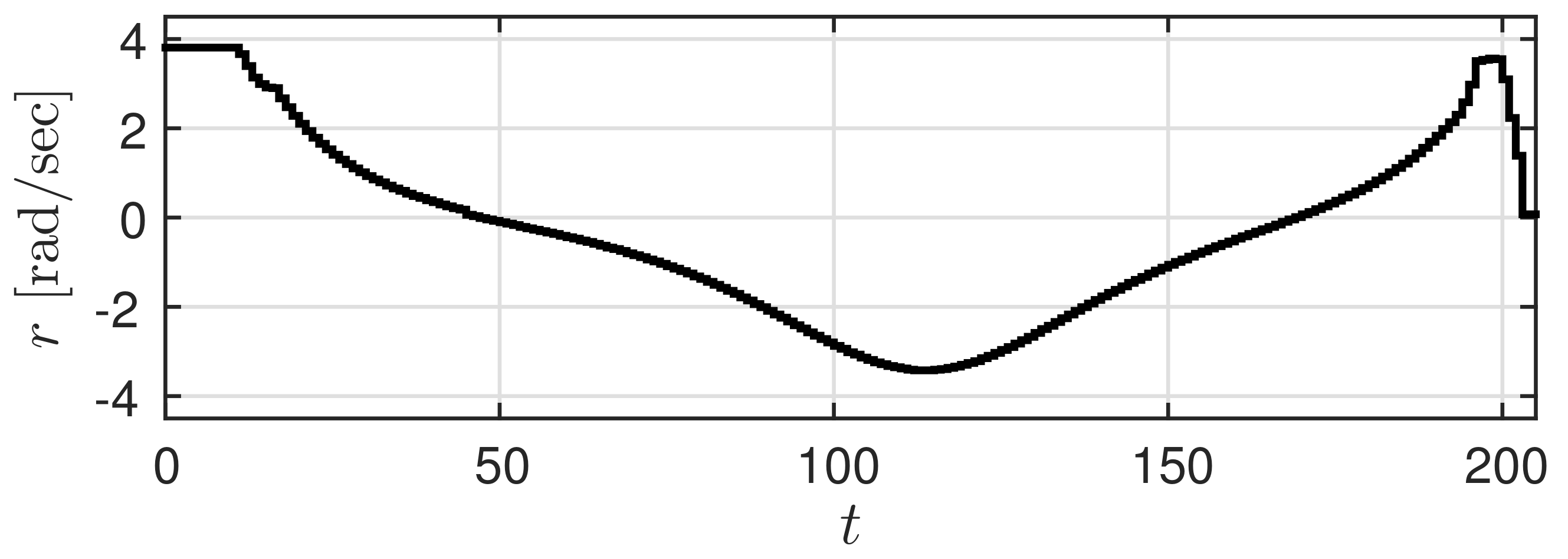
Figure 4.
High accuracy predicted value .

Figure 5.
Time response with prediction governor .
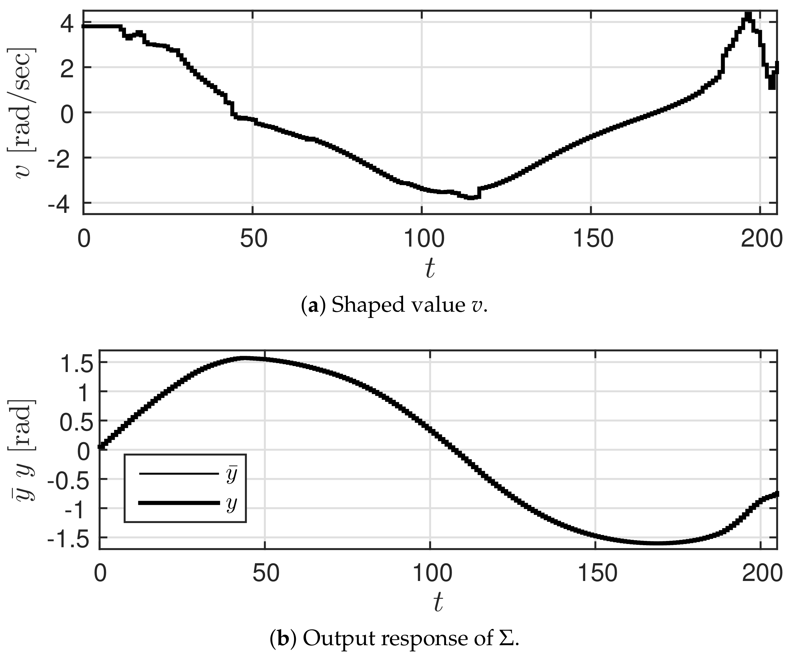
Figure 6.
Time response with predicted value r.

Figure 7.
Trajectory of four-wheel car.
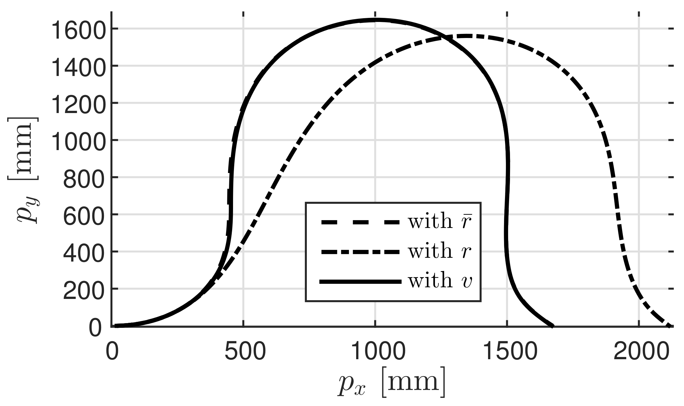
Figure 8.
RoboCar 1/10.

Figure 9.
Experimental setup.

Figure 10.
Proposed shaping strategy by prediction governor.

Figure 11.
Steering angles calculated from predicted value r and shaped value v.

Figure 12.
Trajectory of four-wheel car.

Table 1.
Specification of the RoboCar.
| Item | Specification | |
|---|---|---|
| Body | Size, weight | 190 × 429 × 150 (mm), 2.2 (kg) |
| Minimum turning radius | 500 (mm) | |
| maximum speed | 10 (km/h) | |
| Motor | Drive: Small DC motor, Steering: Servomotor for robot | |
| External sensor | USB camera (640×480 (pix), 30 (fps), 128 (deg)) | |
| Inner Sensor | Rotary encoder | |
| CPU | Intel Celeron Quad Core 1.83 (GHz) | |
| Software | OS | Linux (Ubuntu 14.04) |
© 2018 by the authors. Licensee MDPI, Basel, Switzerland. This article is an open access article distributed under the terms and conditions of the Creative Commons Attribution (CC BY) license (http://creativecommons.org/licenses/by/4.0/).
Share and Cite
MDPI and ACS Style
Minami, Y.; Iwai, Y. Prediction Governors for Input-Affine Nonlinear Systems and Application to Automatic Driving Control. Robotics 2018, 7, 16. https://doi.org/10.3390/robotics7020016
AMA Style
Minami Y, Iwai Y. Prediction Governors for Input-Affine Nonlinear Systems and Application to Automatic Driving Control. Robotics. 2018; 7(2):16. https://doi.org/10.3390/robotics7020016
Chicago/Turabian StyleMinami, Yuki, and Yudai Iwai. 2018. "Prediction Governors for Input-Affine Nonlinear Systems and Application to Automatic Driving Control" Robotics 7, no. 2: 16. https://doi.org/10.3390/robotics7020016
Note that from the first issue of 2016, this journal uses article numbers instead of page numbers. See further details here.